ABSTRACT
This study focused on establishing a straightforward process to create a 3D model using
photogrammetric software and drone photography allowing for the extraction of measurements
of structural data from inaccessible locations. The project specified field data collection
techniques, image processing workflow, and methods of measurement extraction that enabled
structural measurements to be taken from the Northeast high wall of the Boone Quarry outside of
Boone, NC. The study established the need for specifically tailored methods for extracting these
data from 3D models in order to compensate for potential biases in the drone data collection
method, as well as illuminated some potential for bias in structural measurements taken manually
in the field. Using this information, projects utilizing drone imaging and photogrammetry will be
able to design their data collection in a way that corrects for some of these biases and ensures a
more complete data set of structural features.
1. INTRODUCTION
1.1. Background Information
Obtaining structural measurements has historically been limited to sites directly
accessible for the use of a Brunton compass or other manual method; however, advances in
photogrammetry, a process of combining multiple photos into a single image, have made
possible the extraction of measurements from previously inaccessible locations. Photogrammetry
be taken. Software that provides this function often utilizes structure from motion (SFM)
algorithms, which find common points in overlapping images and compute the X, Y, and Z
coordinates for the points using the camera position, orientation, and focal length (Tavani et al.,
2016). Using the point clouds generated from the coordinates, a mesh is then constructed in the
form of irregular triangles and the images are draped over this mesh to produce a photorealistic
3D model (ibid.). Multiple studies have been done to assess the accuracy of image-based models
and have found that they are comparable to LiDAR-based models, which are often cost and size
prohibitive, making them an ideal alternative for many researchers (Tavani et al., 2014). Using a
GPS device, compass, camera, tape measure, and marking tape, and an unpiloted aerial vehicle
(UAV), a 3D model can be produced and structural measurements extracted. The goal of this
study is to determine the optimal workflow for photogrammetric modeling using Agisoft
PhotoScan Professional Edition 1.4, and the extraction of structural data from the model using
CloudCompare 2.9.
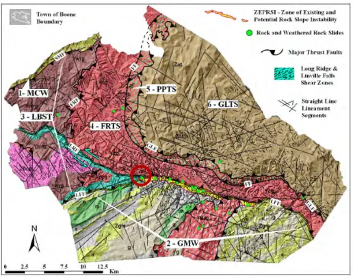
1.2. Geologic Setting
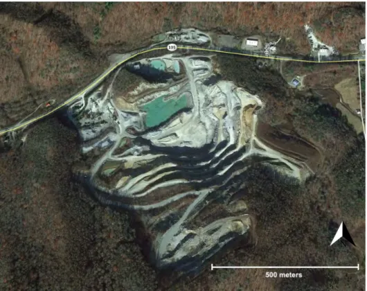
The site selected for this study was the Boone Quarry in Watauga County, North Carolina
(Fig. 1 & 2). The Boone Quarry is located outside of the town of Boone in the Blue Ridge
province in the southern Appalachian Mountains. The area that is now Watauga County was part
of the supercontinent Rodinia at the end of the Mesoproterozoic (Gillon et al., 2009). When
clastic and carbonate sediment deposits and this was followed by the Taconic Orogeny (Middle
Ordovician), during which arc accretion and regional metamorphism and deformation occurred
(ibid.). A final continent-continent collision occurred in the Permian, leading to the formation of
the thrust sheets that compose the Appalachian Mountains and it was this final tectonic event that
produced many of the structures and fabrics observable in Watauga County today, such as shear
zones comprised of bedrock that has undergone mylonitization, folding, faulting, and cataclasis
(ibid.).
Figure 2: Map of Watauga county showing geologic units and lineaments. (Gillon et al., 2009)
The Boone Quarry is located within the Grandfather Mountain Window (GMW) and has
exposures of the Linville Falls Fault (LFF). The GMW is a structural window that exposes the
Late Proterozoic (~765–740 Ma) Grandfather Mountain Formation, which is composed of
greenschist-grade metasandstone, metasiltstone, meta-arkose, and metaconglomerates as well as
interlayered mafic and felsic volcanics (Gillon et al., 2009). The LFF is a thrust fault with a shear
zone several hundred meters thick composed of mylonite, ultramylonite and phyllonite
originating from the Late Mesoproterozoic basement rocks and overprinted with cataclasites
(ibid.) as well as quartzite, meta-arkose, metaconglomerates, and granitoid bodies (ibid.). The
Boone Quarry is located within a region that has been a primary subject of research for the
measurements obtained from this study will be used to supplement ongoing research projects by
faculty and graduate students.
Figure 3: Image taken from Google Earth 4/17/2018
2. METHODS
2.1 Field Data Collection
Field data collection involves three steps: material preparation, setting of ground control
points, and image capture.
Materials needed for field data collection include the following: a compass with built-in
level, a minimum of three ground-control markers, a DJI Phantom quadcopter drone with
mounted camera, a GPS device, and measuring tape. Ground control markers used for this
project were made from pink marker tape placed within the study area. Alternative options
include Jacob staffs or pre-made markers automatically recognizable by PhotoScan and available
for purchase.
2.1.2 Setting Ground Control Points
Correct placement and measurements of Ground Control Points (GCPs) are crucial for
accurately constructing a 3D model. Three types of GCPs should be setup within the site. First,
multiple GCPs should be spread throughout the site all at the same elevation; these will be used
to level the model. Second, GCPs giving specific directional orientation should be placed. At the
Boone Quarry site, a make-shift compass was created by laying marker tape in straight lines
running from North to South and from East to West. Lastly, GCPs are used to scale the model.
Measurements of the marker tape from North to South and from East to West were taken and
used to scale the model.
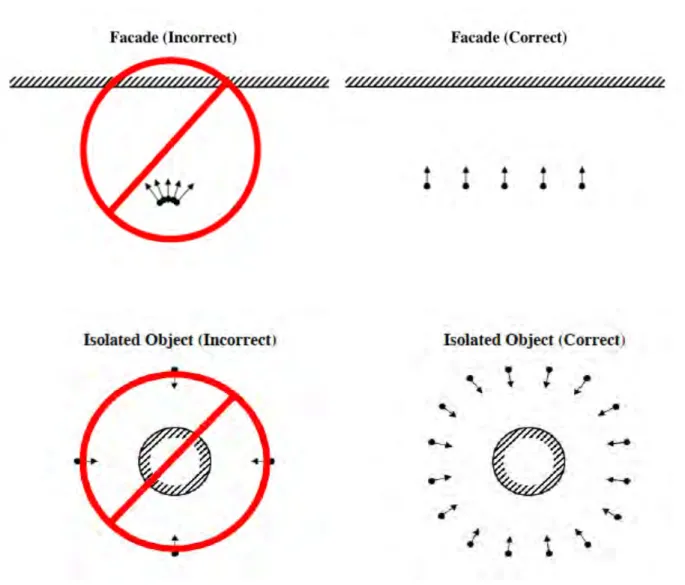
2.1.3 Capturing Photos
one marker are recommended. Do not adjust the focal length while taking pictures and take all
photos in the same lighting conditions. Follow the appropriate diagram below to organize your
photo capture (Fig. 2). 50% overlap minimum is required for model processing. If using UAV
photography, take photos from differing elevations. It is also recommended to take images from
different distances, capturing both a general overview and closer details, in order to have high
enough resolution for structural measurements.
2.2 Image Processing
Image processing is the most time-consuming step in this method. PhotoScan will create
point clouds using the SFM algorithm to find matching points in the images and will assign them
coordinates based on camera position, orientation, and focal length. Next a mesh will be
constructed and images overlain to create the final 3D model. This model will then have to be
exported in order to extract structural measurements as PhotoScan does not have this capability
at this time. Many of the steps in this workflow were informed by the Agisoft PhotoScan
beginners tutorial (http://www.agisoft.com/support/tutorials/beginner-level/), modified for the
purposes of this study.
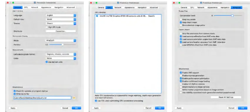
2.2.1 Setting Preferences
To set up PhotoScan preferences on the task bar select PhotoScanPro, Preferences. In the
General tab, specify the directory where your project will be stored (keep the PhotoScan project
and all the images together in one folder). Ensure that if the program detects GPUs that they are
checked in order to enable faster processing. For Mac computers, installation of a CUDA driver
may be necessary in order to utilize built-in GPUs. In the Advanced tab, ensure that Keep depth
maps is enabled to allow for faster processing if any changes are made and it needs to be built
Figure 5: Screen shots of PhotoScan Preferences menu showing settings used in construction of the model
2.2.2 Uploading Photos and Metadata
Before loading pictures, delete any unnecessary or flawed images (i.e. images not of area
of interest, blurry images, changing lighting conditions, moving objects, etc.) to minimize
processing time. Load pictures using Add Photos from the Workflow menu. The pictures
will be loaded in as a “chunk” and will be visible in the Workspace pane. Images will also load
in the Photos pane.
Verify that camera information was loaded automatically by selecting the Reference tab
at the bottom of the Workspace tab. There are three sections in the Reference pane: Cameras,
Markers, and Scale bars. The values to the right of each camera listed should be populated. If
import CSV file, open References pane toolbar and click Import. Select file containing
camera positions. If EXIF does not import automatically, select Import EXIF button. If
the data is in a global or spherical coordinate system it can be converted, using the button at the
top of the references pane, into a projected coordinate system . This is preferable for
exporting and using in CloudCompare. For the creation of this model, the drone measurements
were recorded degrees, seconds, minutes format and was converted into UTM in PhotoScan.
2.2.3 Setting Camera Parameters
In Reference settings, select coordinate system and set the following
accuracies: Camera accuracy (m): 10, Camera accuracy (deg): 50, Projection accuracy: 0.1, Tie
point accuracy: 1. PhotoScan automatically estimates the camera parameters using the EXIF
data. If values are missing they can be added in manually by selecting Tools, Camera calibration
(Fig. 4). After photos have been imported and the camera calibrated the photos can then be
Figure 6: Screen shots of reference settings menu and camera calibration menu in PhotoScan
2.2.4 Aligning Photos
Align photos from the Workflow menu. Set the accuracy at high (medium recommended
for over 100 photos) and genericpreselection enabled. Alternatively, reference preselection can
be used when ground control points are utilized to align the photos, but generic worked for any
model that we processed and no difference was observed in processing time (Fig. 5).
The photo alignment creates a “sparse point cloud” model and will be shown in the
Model view (Fig. 6). This sparse point cloud is made from points selected in the overlapping
portion of images and assigned an x,y,z coordinate where the point is then placed. At this point,
if any photos do not align they can be aligned manually by placing markers on the images and
aligning them to images that were able to align automatically. The Boone Quarry model aligned
on the ground that had no discernable overlapping features and was not ultimately important for
the model and was subsequently deleted.
Figure 7: Screen shot of align photos menu in PhotoScan
After any adjustments are made, it is recommended that optimization is run on the
cameras. This can achieve a higher level of accuracy if any substantial changes were made such
as manually aligning photos (Fig. 7).
Once the sparse cloud optimization is finished, extraneous data should be removed from
the model (i.e. foliage, excess area not needed in model, any objects that moved during imaging).
This can be done in a number of ways. PhotoScan automatically creates a bounding box around
the model which can be moved or resized. Only what is contained within the bounding box will
be used in the reconstruction of the dense point cloud. Resize the bounding box to contain only
the area to be reconstructed. To clean up additional features, the selection tools along the toolbar
can be used to highlight areas and delete them from the model.
For the Boone Quarry model, the edges of the wall were jagged after the point clouds
were built. The bounding box was resized and the selection tool used to smooth edges where
resizing the bounding box was not sufficient to clean up the edges of the model.
2.2.6 Setting Orientation and Scale
By double clicking on a photo that includes one of the GCP markers and the image will
expand allowing a marker to be placed on the GCP in the image. Once a marker has been
created, right clicking on the same ground control point in another photo will provide a
drop-down menu that will allow for placement of any created markers or give the option of creating a
new one. Once a marker has been added to one or two photos, PhotoScan will recognize it and
will automatically place it in the other photos, this will be indicated by a blue flag or gray
symbol appearing over the photo in the photos pane (Fig. 8). Once all markers are placed the
scale bars can be created.
Figure 8: Screen shot showing icons over image in PhotoScan
Create a scale bar by using shift-click to select two markers at a time, right clicking, and
selecting Create Scale Bar. Enter the GPS coordinates for each marker and the distances
between each for the scale bars.
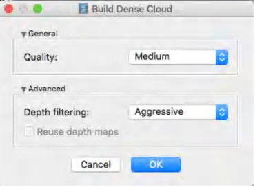
Building the dense point cloud is the most time consuming part of the processing. Prior to
building it, ensure no other programs are running on the computer and check settings to make
sure no interruptions occur during the processing. For example, if the computer automatically
sleeps after a certain amount of time, the processing slows or stops and the program will show
that it has days left of processing. While a data set could potentially take days to process,
depending on the size of the model being constructed it should not take more than 20–30 hours
with smaller models taking significantly less time.
PhotoScan calculates depth information for each image and creates a new “dense point
cloud” model. Medium quality is acceptable for this use, higher quality will take much longer
and is not necessary for finalizing the model for export. Depth filtering should be set to
Aggressive or, if greater than 100 images are used, Moderate can be used. Enable Reuse depth
maps if available to use stored depth maps from earlier processing of the model(Fig. 9). Once
the dense point cloud has completed (Fig. 10) the mesh can be built.
Figure 10: Screen shot of dense point cloud model in PhotoScan
2.2.8 Build Mesh
The mesh should be built using the dense point cloud as the source and the surface type should e
set to arbitrary. Under advanced settings make sure Interpolation is enabled (Fig. 11).
If necessary, faces can be removed from the model after the mesh is built by using the
selection tools from the toolbar and deleting the unwanted faces.
At this point, if the model has any holes, the Close Holes function can be used from the
Tools, Mesh menu. The slider indicates percentage of the total model size that determines the
size of the largest hole to be closed. As the slider is moved, the holes that will be filled display
2.2.9 Build Texture
The final step in the creation of the model is building the texture. Use the mosaic
blending mode and enable hole filling for processing. This step drapes the original images over
the wireframe mesh which creates the final, photorealistic model.
2.2.10 Exporting the model
One issue that occurs when exporting from PhotoScan is that even when the model itself
is correctly oriented, PhotoScan has it saved in its own arbitrary coordinate system and if this is
not fixed prior to export, it will load in this coordinate system in any subsequent program that
opens it. There is a quick fix using a Python script provided by Agisoft on Github
(http://wiki.agisoft.com/wiki/Coordinate_System_to_Bounding_Box.py) that will set the
coordinate system of the program to that of the model bounding box which will allow the model
to export correctly to be used in another program for extracting measurements (see Appendix A).
Save the Python script and then from the tools menu select Run Script. Simply select the file with
the script and execute it. From the File menu, select Export Model and export it as a Wavefront
OBJ (*.obj) file.
2.3 Extracting Structural Measurements
Measurements will be taken using CloudCompare (http://cloudcompare.org), an open
source model editing program, and by utilizing R or Matlab to find a best fit plane to data points
on structural features. An alternative open source program for extracting structural data is
OpenPlot which has been utilized in other studies of 3D model measurements (Tavani et al.,
2.3.1 Importing the model into CloudCompare
Depending on the size of the model CloudCompare may recommend a shift in the
coordinate system when the obj. file is opened. This is done to preserve the original precision of
the model. The original coordinate system is restored when the model is saved or exported. Since
the shift is consistent across all points it does not affect the orientation data that is extracted from
the model (Fig. 13).
Figure 13: Screen shot of model imported into CloudCompare
2.3.2 Picking points
In the DB Tree toolbar on the left-hand side, click the drop down on the model folder and
vertices box is checked, if it is not enabled no measurements are able to be taken. The vertices
will be shown in the model as points.
Figure 14: Screen shot of DB Tree menu in CloudCompare
Using the point list picking tool select at least three points for each structure. These will
populate the point list, but they will not be named, so the number of points per feature must be
tracked either manually or by starting a new point list for each feature (Fig. 15). Using the save
button on the point list picking toolbar the points can be saved as a CSV file and loaded into
2.3.3 Fitting a plane to the points
The University of Georgia’s stratigraphy lab provides an R code
(http://strata.uga.edu/forms/strikeDipRotation.r) for fitting a plane to points picked from the
model using least squares minimization (see Appendix A). This code takes a set of points and
calculates a plane such that the sum of the squared errors is minimized. This code also includes a
function for removing the dip in order to reestablish original horizontality of dipping layers
which was not used for this study.
The outputs from the code give strike, dip and dip direction in azimuth for the planes. In
order to visually assess the orientation, a plane can be created in CloudCompare and placed into
the model using the dip angle and dip direction as well as the coordinates of one of the points
taken from the plane (Fig. 16). From the toolbar select edit, plane, create. This will open a plane
properties dialog box where the measurements for the plane can be added (Fig. 17).
Figure 17: Screen shot of plane properties menu in CloudCompare
2.3.4 Additional uses for model
The model is capable of being saved as a KML file and exported into Google Earth. More
details regarding this are discussed in Tavani et al. (2014).
3. RESULTS
A total of 306 photos of the Boone Quarry site were taken by drone and 11 GCPs were
placed on site. Upon import into PhotoScan 305 of the 306 photos were successfully aligned, the
were identified in the photos and in the model using markers. GPS coordinates of the GCPs were
specified and scale bars were created using the North-South and East-West markers and
specifying the distances between. The mesh was generated resulting in 4,406,609 faces and
2,205,993 vertices. At this point the PhotoScan orientation was set to the bounding box
coordinate system by running the Python script in the console in PhotoScan, the texture was
generated, and the model exported.
The exported model was next opened in CloudCompare. Using original photos as guides
for selection, three to four points were selected from 40 structural features including faults and
fractures on the model (Fig. 18). These points were exported into an Excel spreadsheet and then
into R. Using the R code from UGA, planes were fitted to the 40 structural features including
joints and faults giving the strike, dip, and dip direction for each plane.
Figure 18: Drone image of Northern-most section of the high wall that was modeled. Joints and minor faults that were measured are indicated by red lines.
Results were visually assessed by creating planes in CloudCompare and placing them in
the model space to verify appropriate alignment. The data were then inputted into Stereonet
developed by Rick Allmendinger at Cornell University and Nestor Cardozo at the University of
Stavanger, Norway (2013). Planes as well as poles to planes were plotted and contours were
added to visualize distribution of structural features (Fig. 19). The poles to the planes taken from
the model show that the largest concentration of the planes measured strike in a North-South
direction with a smaller number of East-West striking structures.
These data were then compared to measurements of faults taken inside the quarry by the
North Carolina Geological Survey (NCGS, 2007), measurements of fractures taken at an outcrop
immediately outside the entrance to the quarry, and measurements of fractures taken at another
nearby outcrop (Hill, 2018). The NCGS fault data shows the primary orientation striking in the
East-West direction (Fig. 20). The two data sets taken of fractures outside of the quarry also give
the primary orientations of fractures as striking East-West (Figs. 21 & 22).
Figure 19: Drone Model joint and minor fault measurements of Boone Quarry
Figure 21: Joint measurements taken on outcrop immediately outside the entrance to the Boone Quarry by Jesse Hill
Figure 22: Joint measurements taken 900 meters west of Boone Quarry off of Hwy 105, across from concrete plant by Jesse Hill
4. DISCUSSION
The measurements taken using the drone/3D model technique resulted in a data set that is
different from the NCGS data set as well as the other measurements taken in the nearby areas.
There are a few possible explanations for why this occurred. The NCGS measurements were
collected from different locations throughout the quarry indicated on the figure by the red dots,
with a higher concentration being taken from the Southeast walls, whereas the wall that was
imaged by the drone was the Northeast high wall as indicated by the red rectangle (Fig. 23).
There are also different geologic units present within the quarry which could explain differences
in orientations of structural features. The NCGS noted that the dips of the layering in the quarry
steepened towards the Southwest which shows that there are changes in orientation based on
Figure 23: Locations of measurements taken by NCGS with red dots indicating fault measurements. The red rectangle shows the location of the constructed 3D model from the drone imaging.
Furthermore, it is possible that different measurement techniques may have biases that
are affecting the data that is collected. For example, field measurements may be subject to an
inherent bias towards faults and features that strike perpendicular the face of an exposure, which
are more visible to on-site surveyors facing an outcrop or wall, while planes running parallel to
the face are less obvious and may consequently be missed during measurement. Measurements
parallel to one another strike at high angles to the face, many measurements of the same
orientation may be taken from these joints increasing the frequency of that orientation in the data
set, however, if they run parallel to the face, only one joint from the set will be exposed and there
will be a lower frequency of measurements taken from that orientation. Considering these
factors, it is reasonable to assume that there is some bias inherent in the method of data
collection which would lead to field measurements having higher frequency and increased
likelihood of recording features striking at high angles to the whereas there would be a higher
likelihood of measuring features parallel to the face when extracting data from the 3D model.
Based on this, we would expect to see measurements from the high wall of the Boone Quarry
which is oriented North to South to show a prevalence of North to South striking features which
is which is consistent with our data.
There are potential solutions that could resolve this issue. One method for obtaining more
varied measurements from a site with a single orientation would be to create a separate 3D model
comprised of images taken at a closer distance to the structural features which can provide more
detail and result in a model that retains more of the 3D data. This model could then be oriented to
the larger model and measurements could be obtained of the features with less exposure.
Secondly, the potential bias of obtaining measurements from a 3D model could be overcome
with deliberate planning of image collection. By selecting differently oriented exposures from
which to extract data, the inherent bias could be corrected for and resulting data would be more
balanced.
Overall, the primary limitation of this method was the time it took to process the images,
which was not prohibitive. Additionally, the need for multiple programs and code-fixes makes
entire workflow. Another possible limitation could be the cost of the drone and the PhotoScan
software, but barring these two expenses the method is very cost-effective.
The primary purpose of this study was to determine a protocol for creating 3D models
using photogrammetry that would allow for structural measurements to be taken from
inaccessible sites, however, this methodology has the potential to open up other new possibilities
for field work processes. Instead of relying on sketches of outcrops taken in the field, it is now
possible to bring the outcrop back virtually and to access it for further study or for educational
purposes. Another benefit of this method is the ability to view the study area from differing
orientations which helps to enhance the overall understanding of the structural features that are
present. By utilizing materials available to most researchers, this method can obtain reliable
measurements with little added cost making it an appealing option when standard field methods
are restricted due to inaccessibility of structural features. In conclusion, photogrammetry is a
suitable alternative for standard field methods that produces reliable results with nominal
additional time or expenses and will certainly become a standard practice for researchers moving
forward.
ACKNOWLEDGEMENTS
Thank you to my thesis advisor Dr. Kevin Stewart for his guidance and support during
this project. Thank you to Jesse Hill for assisting me with many steps in this process from simple
5. APPENDIX A: SUPPLEMENTARY DATA
R CODE
planeForPoints <- function(x, y, z) {
# Source - http://www.sci.utah.edu/~balling/FEtools/doc_files/LeastSquaresFitting.pdf # 3 Planar Fitting of 3D Points of Form (x,y,f(x,y))
# returns column vector [A, B, C], where z = Ax + By + C
xi <- sum(x) yi <- sum(y) zi <- sum(z) xi2 <- sum(x^2) yi2 <- sum(y^2) xiyi <- sum(x*y) xizi <- sum(x*z) yizi <- sum(y*z) n <- length(x)
M1 <- matrix(data=c(xi2, xiyi, xi, xiyi, yi2, yi, xi, yi, n), nrow=3) M2 <- matrix(data=c(xizi, yizi, zi), nrow=3)
solution <- solve(M1, M2) return(solution)
}
rSquaredPlane <- function(x, y, z, plane) {
# plane is the output of planeForPoints(), a column vector [A, B, C], # where z-hat = Ax + By + C
zHat <- plane[1]*x + plane[2]*y + plane[3] SSE <- sum((z-zHat)^2)
SST <- sum((z-mean(z))^2) Rsquared <- 1 - SSE/SST Rsquared
}
vcrossprod <- function(a, b) {
# returns line that forms intersection of two planes a and b # returns column vector [x, y, z] of the line in three dimensions c1 <- a[2]*b[3] - a[3]*b[2]
c2 <- a[3]*b[1] - a[1]*b[3] c3 <- a[1]*b[2] - a[2]*b[1]
c <- matrix(c(c1, c2, c3), nrow=3) return(c)
}
# converts angle theta on a unit circle to compass azimuth
# - unit circle has origin at 90° on compass with values increasing counterclockwise # - need origin at 0° on compass with values increasing clockwise
# input and output are in degrees, not radians azimuth <- 450 - theta
if (azimuth > 360) { azimuth = azimuth - 360 }
return(azimuth) }
strike <- function(a) {
# returns the azimuth of the strike (in degrees) of plane a
# where strike is the intersection of plane a and the horizontal plane. # uses east-half rule (i.e., strike is always 0-180°)
horizontalPlane <- matrix(data=c(0,0,1), nrow=3) strikeLine <- vcrossprod(a, horizontalPlane) theta <- atan(strikeLine[2]/strikeLine[1]) * 180 / pi azimuth <- azimuthFromUnitCircle(theta)
return(round(azimuth, 1)) }
dipDirection <- function(a) {
# returns the azimuth of the dip direction (in degrees) from plane a strikeAzimuth <- strike(a)
xSlope <- a[1] ySlope <- a[2]
dipAzimuth <- strikeAzimuth if (xSlope > 0) {
if (ySlope >= 0) {
dipAzimuth <- strikeAzimuth - 90 # SE dip } else {
dipAzimuth <- strikeAzimuth + 90 # NW dip }
} else {
if (ySlope > 0) {
dipAzimuth <- strikeAzimuth - 90 # SW dip } else {
dipAzimuth <- strikeAzimuth + 90 # NE dip }
}
xSlope <- a[1] ySlope <- a[2]
if (xSlope == 0) { # add negligible amounts to prevent dividing by zero xSlope <- 0.000001
}
if (ySlope == 0) { ySlope <- 0.000001 }
alphaX <- atan(xSlope) alphaY <- atan(ySlope)
dipRadians <- atan(tan(alphaX) * sqrt(tan(alphaY)^2 / tan(alphaX)^2 + 1)) dipDegrees <- dipRadians * 180 / pi
if (dipDegrees < 0) {
dipDegrees = - dipDegrees }
return(round(dipDegrees, 1)) }
######## dip degrees and dip direction
PYTHON SCRIPT
# Rotates model coordinate system in accordance of bounding box for active chunk. Scale is kept.
#
# This is python script for PhotoScan Pro. Scripts repository: https://github.com/agisoft-llc/photoscan-scripts
import PhotoScan import math
# Checking compatibility
compatible_major_version = "1.4"
found_major_version = ".".join(PhotoScan.app.version.split('.')[:2]) if found_major_version != compatible_major_version:
raise Exception("Incompatible PhotoScan version: {} != {}".format(found_major_version, compatible_major_version))
def cs_to_bbox():
print("Script started...")
R = chunk.region.rot # Bounding box rotation matrix C = chunk.region.center # Bounding box center vector
if chunk.transform.matrix: T = chunk.transform.matrix
s = math.sqrt(T[0, 0] ** 2 + T[0, 1] ** 2 + T[0, 2] ** 2) # scaling # T.scale() S = PhotoScan.Matrix().Diag([s, s, s, 1]) # scale matrix
else:
S = PhotoScan.Matrix().Diag([1, 1, 1, 1])
T = PhotoScan.Matrix([[R[0, 0], R[0, 1], R[0, 2], C[0]], [R[1, 0], R[1, 1], R[1, 2], C[1]],
[R[2, 0], R[2, 1], R[2, 2], C[2]], [ 0, 0, 0, 1]])
chunk.transform.matrix = S * T.inv() # resulting chunk transformation matrix
print("Script finished!")
label = "Custom menu/Coordinate system to bounding box" PhotoScan.app.addMenuItem(label, cs_to_bbox)
6. REFERENCES CITED
Agisoft LLC, 2017, coordinate_system_to_bounding_box.py: A code that will rotate model coordinate system in accordance of bounding box for active chunk, Agisoft LLc, St. Petersburg, Russia, Retrieved from: https://github.com/agisoft-llc/photoscan-scripts/blob/master/src/coordinate_system_to_bounding_box.py.
Agisoft LLC, 2017, PhotoScan Professional: a stand-alone software product that performs photogrammetric processing of digital images and generates 3D spatial data: Agisoft LLC, St. Petersburg, Russia
Agisoft LLC, 2018, Tutorial (Beginner Level): Orthomosaic and DEM generation with Agisoft PhotoScan Pro 1.3 (without ground control points),
http://www.agisoft.com/pdf/PS_1.3%20-Tutorial%20(BL)%20- %20Orthophoto,% 20DEM%20(without%20GCPs).pdf (accessed April 2018).
Allmendinger, R. W., Cardozo, N. C., and Fisher, D., 2013, Structural Geology Algorithms: Vectors & Tensors: Cambridge, England, Cambridge University Press, pp. 289
Cardozo, N., and Allmendinger, R. W., 2013, Spherical projections with OSXStereonet: Computers & Geosciences, v. 51, no. 0, p. 193 - 205, doi: 10.1016/j.cageo.2012.07.021
Hill, J., Stewart, K., 2016, A newly discovered fault zone near Boone, North Carolina and Cenozoic topographic rejuvenation of the southern Appalachian mountains, in
Proceedings, GSA Annual Meeting in Denver: Colorado, USA, 2016, Geological Society of America, Abstracts with Programs, v. 48, n. 7, doi: 10.1130/abs/2016AM-283940
Gillon, K.A., et al., 2009, Integrating GIS-based geologic mapping, LIDAR-based lineament analysis and site specific rock slope data to delineate a zone of existing and potential rock slope instability located along the Grandfather Mountain Window-Linville Falls shear zone contact, Southern Appalachian Mountains, Watauga County, North Carolina,
in Proceedings, US Rock Mechanics Symposium, 43rd, and U.S.-Canada Rock Mechanics Symposium, 4th, Asheville: North Carolina, North Carolina Geological Survey
Girardeau-Montaut, D., 2018, CloudCompare: a 3D point cloud and mesh processing software: CloudCompare.org, Open Source Project, http://cloudcompare.org.
North Carolina Geological Survey, PDF of report of fault measurements taken inside Vulcan Boone Quarry on May 23, 2007, acquired through personal communication with Jesse Hill, 2018.
Tavani, S., Corradetti, A., and Billi, A., 2016, High precision analysis of an embryonic extensional fault-related fold using 3D orthorectified virtual outcrops: The
Tavani, S., Granado, P., Corradetti, A., Girundo, M., Iannace, A., Arbués, P., Muñoz, J.A., and Mazzoli, S., 2014, Building a virtual outcrop, extracting geological information from it, and sharing the results in Google Earth via Openplot and Photoscan: An example from the Khaviz anticline (Iran): Computers & Geosciences, v. 63, p. 44-53,
doi:10.1016/j.cageo.2013.10.013.
UGA Stratigraphy Lab, 2016, Plane from points: R code to fit a plane to a set of points picked on a 3-d model obtained from drone-based photogrammetry and calculate the strike and dip of that plane, University of Georgia Stratigraphy Lab,