Weak gravitational lensing in the red-sequence cluster survey 2

(1)

The handle http://hdl.handle.net/1887/19026 holds various files of this Leiden University

dissertation.

Author

: Uitert, Edo van

(2)

Weak gravitational lensing in the Red-sequence

Cluster Survey 2

(3)

(4)

Weak gravitational lensing in the Red-sequence

Cluster Survey 2

Proefschrift

ter verkrijging van

de graad van Doctor aan de Universiteit Leiden,

op gezag van de Rector Magnificus prof. mr. P. F. van der Heijden, volgens besluit van het College voor Promoties

te verdedigen op dinsdag 29 mei 2012 klokke 13:45 uur

door

Edo van Uitert geboren te Groningen

(5)

Promotor: Prof.dr. K. H. Kuijken

Co-Promotor: Dr. H. Hoekstra

Overige leden: Prof.dr. M. Franx Prof.dr. J. Schaye

(6)

Voor saba&safta, opa&oma

(7)

(8)

1

Introduction

In this first chapter, we set the scene for the research projects presented in this thesis. We begin with a brief description of the standard model of cosmology, ΛCDM, and describe its main components. To study these observationally, a large variety of techniques has been developed. The one central to the studies in this thesis is weak gravitational lensing. We therefore provide a short description of how this method works, and give some examples of its applications. We also provide a short overview of the other chapters.

1.1 The

Λ

CDM framework

For millennia, people believed that the Earth was the centre of the Universe, with the Sun, the planets and all the stars revolving around it. Almost 500 years ago, this ancient world view started to change, and it has been subject to change ever since. Due to the work of, amongst others, Nicolaus Coperni-cus and Galileo Galilei, it became clear that our Sun did not revolve around the Earth, but that the Earth and the planets moved around the Sun. At the same time, Giordano Bruno proposed that the stars in our sky were actually very distant suns like our own, although it took more than two centuries before their distances from us could be determined. With the help of his telescope, Galileo Galiliei found that the faint band of light that crossed our nocturnal sky actually consisted of many small stars our eyes could not discern. This large collection of stars was called our Galaxy, and at the beginning of the twentieth century it was a hot topic of debate whether or not other galaxies similar to ours existed outside our own. In the 1920s, Edwin Hubble measured the distances to some faint nebulae in the sky whose origin was uncertain. These distance measures conclusively showed that these objects had to reside far outside our Galaxy, and therefore had to be galaxies themselves. Subsequent observations showed that the Universe was filled with uncountable galaxies - currently, it is estimated that there are more than 100 billion of them.

(11)

as it was astonishing: it could only mean that all galaxies were moving away from each other, hence the Universe was expanding. Until then, the Universe had been thought to be static. If it was expanding, it meant that it had a be-ginning as well. This moment when everything was created has become famous as the Big Bang (the name was coined by Fred Hoyle in 1949, who believed in a static Universe and invented the term to sarcastically express his dislike in the theory - although according to his reading, the term only served to highlight the differences between the theories). The fact that people had great difficulties in believing in a Universe that was not static but expanding was demonstrated by one of the greatest minds of all times, Albert Einstein. In his work on General Relativity a few years earlier, he added a constant to one of his equations so that it would enforce a static Universe rather than an expanding one (the largest error of his career, he later confessed, as he could have predicted the expansion of the Universe before it was observed).

Another change of our world view was initiated in the 1930s by the work of Fritz Zwicky on groups of galaxies (galaxy clusters), but only became widely known after the work of Vera Rubin and her collaborators in the 1960s. Zwicky studied the orbital velocities of galaxies in the Coma cluster, and inferred from their large velocities that ‘missing’ mass had to be present to prevent these galaxies from flying off. Rubin studied rotation curves1 of nearby spiral galax-ies and deduced the total mass enclosed within a certain radius using standard Newtonian physics. The total mass exceeded the mass that could be accounted for by the sum of stars, gas and dust (the baryons). Hence another component had to be present, exerting gravity, but invisible to the eye: dark matter. Nowa-days, the presence of dark matter has been confirmed by various observations, including the stellar dynamics in nearby galaxies, the kinematics of satellite galaxies in clusters, and by observations of hot X-ray emitting gas. These ob-servations support the view that the galaxies and galaxy clusters we observe are embedded in giant dark matter structures. One of the most convincing observations supporting the existence of dark matter has been made by Clowe et al. (2006) in a system called the Bullet Cluster. In this work, two galaxy clusters are studied just after they crashed into each other. The hot gas from both galaxy clusters, which constitutes the major part of the ordinary baryonic matter, collided violently and slowed down, whilst emitting a huge amount of X-ray radiation. The dark matter, however, which only interacts through grav-itation, did not collide and moved on after the collision, forming two separate clumps, clearly offset from the gas.

At about the same time of the first observations of galaxy rotation curves, Penzias and Wilson, two radio engineers working for Bell Labs, measured a source of radio noise at millimeter wavelengths coming from all directions in the sky. Radiation in this wavelength regime had already been predicted in 1948 by Gamow, Alpher and Herman as a relic of the Big Bang. Shortly after the Big Bang, the Universe consisted of one giant immensely dense and hot soup of elementary particles and radiation. After approximately 380 000 years of expan-sion and cooling, the conditions in the Universe allowed protons and electrons to recombine and form hydrogen atoms. During this process, photons were emit-ted with an energy of 13.6 eV, i.e. with a frequency peaking in the ultraviolet.

(12)

1.1. THEΛCDM FRAMEWORK

Most of these photons traversed the Universe ever since, although the expan-sion of the Universe redshifted their frequency to the millimeter regime. This radiation, known as the Cosmic Microwave Background Radiation (CMBR), was exactly what Penzias and Wilson observed. The CMBR is found to be ex-tremely homogeneous, and is very well described by a black-body spectrum with a temperature of 2.71 K, with fluctuations of the order 10−5K. The observation of the CMBR at exactly the expected wavelength regime is considered as one of the strongest proofs that the Big Bang actually happened. Detailed observa-tions of the CMBR pattern across the sky with, amongst others, the Wilkinson Microwave Anisotropy Probe (WMAP) space telescope (Bennett et al. 2003; Jarosik et al. 2011) revealed a wealth of information about the structure of the Universe (e.g. that space appears flat rather than curved). It also provided constraints on the total amount of matter in the Universe, as well as strong evidence that a large fraction of the matter in the Universe has to be in a non-baryonic form (i.e. dark matter). The extreme homogeneity of the CMBR is commonly attributed to a period just after the Big Bang when the Universe expanded extremely rapid - exponentially - for a short timespan, which is called inflation. During inflation, the tiny quantum fluctuations in the Universe were blown up, and formed the seeds of the structure that formed afterwards.

In 1998, two independent research groups, called the high-z SN search2

and the Supernova Cosmology Project3 determined the distance to very dis-tant galaxies by studying the light of exploding stars (supernovae; Riess et al. 1998; Perlmutter et al. 1999). This lead to the discovery that these distant galaxies are actually more distant than predicted for a Universe that expands at a constant rate. The only explanation again changed our world view radically - not only is the Universe expanding, but the expansion is actually accelerating! This conclusion has been disputed over the years, but the evidence supporting this view is increasing. For example, the CMBR observations show that the Universe is practically flat, which means that the average density in the Uni-verse is close to a particular value (the critical density). Combining this with the constraints on the total amount of matter in the Universe, it follows that an additional form of energy has to be present. Also, studies of the growth of structure point in the same direction (e.g. Schrabback et al. 2010). What is causing this acceleration is not clear, but it is attributed to a hypothetical form of energy: dark energy. The nature of dark energy is not understood at all. Attempts have been made to relate it to the ground state energy of the quantum field that pervades space, but the discrepancy between the theoretical value and the value that follows from cosmological observations is an incredible factor of 10−120_{, which serves as a perfect illustration of our ignorance. These}

four components, i.e. the baryons, radiation, dark matter and dark energy, are currently believed to make up the Universe.

Parallel to all these observations, astronomers have developed countless mod-els to describe our Universe and the way it evolves. Most of these modmod-els were discarded at some point as observations proved them wrong. One of them, however, has managed to stand the test of time so far, and is currently the most favoured model by the majority of the astronomical society. The model is called ΛCDM. The ”CDM” stands for Cold Dark Matter, where the ”Cold”

(13)

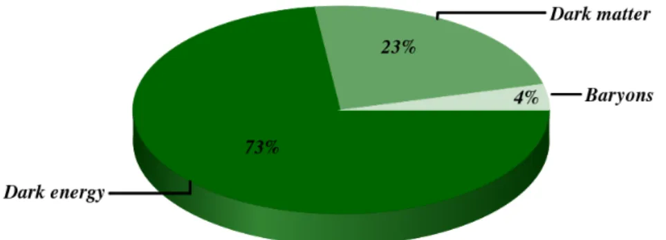
Figure 1.1: Contribution to the total energy density of the Universe by the three main components of ΛCDM.

indicates that the dark matter particles have relatively high masses and move at low speeds (as opposed to Hot Dark Matter, where the particles are assumed to move with relativistic speeds). The Λ refers to the constant Einstein added to his equations to enforce a static Universe, which he considered a mistake, but ironically has been reintroduced as the most natural description for dark energy. The ΛCDM model describes how the Universe, starting from a very hot and dense state, expanded, gradually cooled and eventually formed stars and galaxies. The strength and beauty of ΛCDM is that from a modest number of initial conditions and ingredients, it has the ability to predict with great pre-cision a large variety of observations, ranging from the observations of density peaks in the cosmic microwave background radiation, to the cosmic abundances of the light elements (hydrogen, helium, deuterium and lithium), to the cluster-ing of galaxies in the current day Universe. In ΛCDM, hot dark matter is also present in the form of neutrino’s, but they only make up a small fraction of the total energy budget.

In our Universe, the baryons only make up a very modest part of the total content, as is depicted in Figure 1.1. The two dark components, dark matter and dark energy, dominate the energy density, but their nature is poorly un-derstood at best. The majority of current research in cosmology is aimed at improving our understanding of these components: how are they distributed in the Universe, what are they made of, how do they interact, etc.

(14)

1.2. GRAVITATIONAL LENSING

These processes play, however, a very significant role in the formation of struc-ture, and need to be incorporated accurately. If the implementation of these processes is not correct, neither will be the predictions from the simulations.

Although simulations improve our understanding of the evolution of our Universe, how it came to be as we observe it today, they need to be constrained by observations. For example, when we compare simulations with different implementations of supernova feedback to observations, we can learn which sce-nario is more likely than the other. But the opposite is true as well: for a given set of observations, we need simulations to help interpret what we see. Com-paring observations with the results from simulations is generally complicated. Observations are distorted by all sorts of processes in the intergalactic medium, the atmosphere and the telescope, for which we have to correct. Simulations, however, offer a simplification of reality, as not all the processes that occur in the real Universe are accounted for. To match the observations to simulations and vice versa, we have to translate the one into the other, and herein lies the difficulty. Nonetheless, it is worth the effort as only through the combination of both we can improve our understanding of the Universe.

This thesis is part of the observational effort to study how dark matter is distributed in and around galaxies and galaxy clusters, and how it traces the baryons. The main technique we have used in our studies is gravitational lensing, which we introduce in the following section.

1.2 Gravitational lensing

As light emitted by distant galaxies (sources) travels through the Universe towards our telescopes, it is deflected by the gravitational pull of massive galax-ies and galaxy clusters (lenses) that it passes on its way. Rather than in straight lines, each lightray follows a wiggly path through space. This effect is known as gravitational lensing. A sketch of a gravitational lens system is shown in Figure 1.2. A galaxy at a distance Ds from us that resides in the source plane emits

light rays, that travel towards Earth (depicted by the thick solid line). After traveling the distance Dds, the lightray is deflected by a massive structure in

the lens plane, and travels the remainingDdin a direction that is different from

its original path towards the observer on Earth. This deflection of a lightray is described by the following geometrical relationship:

~

β=~θ−~α(Dd~θ)

Dds

Ds

, (1.1)

withβ~ the angular position of the source,~θthe angular position of the image, and~α(Dd~θ) the deflection angle. Introducing the angular coordinateξ~=Dd~θ,

the deflection angle is given by

~

α(~ξ) = 4G

c2

Z

d2ξ0Σ(ξ~0)

~ ξ−ξ~0

|_ξ~₋_ξ~0_|2 (1.2)

(15)

Figure 1.2: Sketch of a gravitational lens system (Bartelmann & Schneider 2001)

with Σ(ξ~0) the surface mass density and~ξ the impact parameter (Bartelmann & Schneider 2001).

Gravitational lensing affects our observations in several ways. Firstly, the observed location of source galaxies is different from their real positions on the sky. Since we do not know their positions beforehand, we cannot measure this effect. Secondly, if the lens is very massive, the lightrays are bent around different sides of the lens towards Earth. As a result, we may observe more than one image of the same source galaxy. The length of the path that the light travels before it reaches us generally differs between the images. Therefore, when the light emitted by the source suddenly changes (for example due to a supernova explosion), this ‘news’ arrives at Earth for each image at a different moment. These so-called time delays can be used to study the rate of expansion of the Universe (Refsdal 1964), and constrain several cosmological parameters (Coe & Moustakas 2009).

(16)

I(x, y) to the observed one,I0(x0, y0). It is given by:

x0 y0

= (1−κ)

1−g1 −g2

−g2 1 +g1

x y

(1.3)

with (x, y) the observed coordinates and (x0, y0) the undistorted ones. κis the convergence, defined as

κ= Σ(

~ ξ) Σcrit

; Σcrit=

c2

4πG Ds

DdDds

, (1.4)

with Σcrit the critical surface mass density. The weak lensing regime is defined

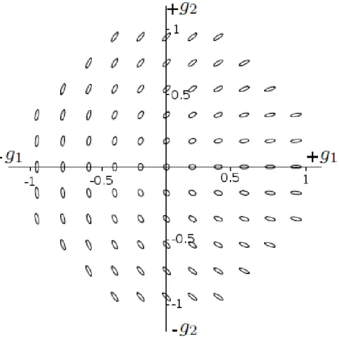
as the regime where κ 1 holds; if κ≥1, Equation (1.1) can have multiple solutions, resulting in multiple images of a single source for particular lens-source configurations. g1, g2≡(γ1, γ2)/(1−κ) is the reduced shear and (γ1, γ2)

the shear. The shear describes the stretch of the image of the source due to the gravitational potential of the lens. Its effect on a round source is illustrated in Figure 1.3. The quantity we measure from the source ellipticities is the reduced shear, however. In weak lensing,κ1, and thereforeg≈γ, hence the reduced shear is approximately equal to the shear. If the distortion is small, it can be shown that the ellipticities of source galaxies change as follows:

eobs_i =eint_i +gi, (1.5) witheobs

i one of the two components of the observed ellipticity, andeinti the

in-trinsic ellipticity of the source. The shear can be retrieved in a certain part of the sky by averaging the ellipticities of a large number of sources: hgii ≈ heobs

i i. The

fundamental assumption made here is that the intrinsic ellipticities of galaxies have random orientations; the intrinsic part of the observed ellipticities aver-ages out, leaving us with the average shear imprinted on those sources. This assumption is actually not correct as neighbouring galaxies that are or have been subject to the same large-scale gravitational field may have correlated el-lipticities, an effect known as intrinsic alignments (e.g. Hirata et al. 2004, 2007). This affects studies that rely on the correlation of the ellipticities, but not the studies where the ellipticities are correlated with the location of the lenses as the lensing signal is generally averaged over large numbers of sources, and the effect averages out.

If a spherically symmetric lens lenses a source, the shape of the source is stretched tangentially, i.e. in the direction perpendicular to the vector that connects the lens with the source projected onto the plane of the sky. To un-derstand this qualitatively, trace the lightrays back past the lens to the source. The lightrays that passed the lens at small impact radii (close to the lens) were deflected more than the lightrays that passed it at larger radii, hence the real image of the source is stretched radially compared to the image we observed. Vice versa, the observed image is stretched tangentially with respect to the real image. This process is illustrated in Figure 1.4.

A commonly used method to extract the shear from the shapes of the sources is therefore by measuring the source ellipticity components in the direction tan-gent to the line that connects the lens and the source, hence the direction in which they were distorted. The quantity we measure is the tangential shear (also known as the galaxy-mass cross-correlation function),

(17)

Figure 1.3: Gravitational shear applied on an intrinsically round source. If g1

is positive (negative), the source is stretched horizontally (vertically); if g2 is

positive (negative), the source is stretched in the x = y (x = −y) direction (source: D. Clowe).

with θ the angle between the horizontal axis and the vector between the lens and the source. By measuring the tangential shear in concentric rings centred on the lens, the radial shear pattern of the lens can be studied.

To determine whether galaxy-galaxy lensing produces a tangential shear that is positive or negative, we imagine a round source galaxy that lies on the hori-zontal axis that passes through the centre of the lens, hence cos(2θ) = 1. The distortion of its shape is in the tangential direction: the source is stretched ver-tically. In Figure 1.3 we find that this corresponds to a negativeγ1. Therefore,

the tangential shear is positive.

The tangential shear is a convenient way to quantify the lensing signal, be-cause it can be directly related to the differential surface mass density:

hγt(ξ)i=

∆Σ(ξ) Σcrit

(18)

Figure 1.4: Cartoon of galaxy-galaxy lensing. Lightrays of a source passing the lens at different impact parameters are bent by different amounts. As a consequence, the shape of the source becomes elongated in the direction per-pendicular to the lens-source separation. When seen in projection on the sky, a coherent shear pattern is formed around the lens when there are multiple sources at different positions behind the lens.

where ∆Σ(ξ) = ¯Σ(< ξ)−Σ(¯ ξ) is the difference between the mean projected surface density enclosed byξand the mean projected surface density on a circle atξ. Since we only measure the difference between projected densities, and not the projected density itself, we can in principle not determine the mass of the lenses, unless we know the value of the projected density at a certain position in the lens plane. In other words, if we were to increase the density uniformly across the lens plane, the tangential shear in the weak lensing regime (κ1) would not change, but the mass obviously would – this problem is known as the mass-sheet degeneracy (Falco et al. 1985; Schneider & Seitz 1995). The most common solution to this problem is to assume a certain two-dimensional profile for the density (e.g. based on results from numerical simulations), and fit the corresponding lensing signal to the observed shear. Amongst the most popular models are the Singular Isothermal Sphere (SIS) profile, and the Navarro-Frenk-White (NFW) profile (Navarro et al. 1996). The total mass is then obtained by integrating the density in an area where the density is larger than a certain threshold value.

(19)

if the luminosity function5_{of a certain sample of sources is accurately known,}

the effect is measurable (e.g. Hildebrandt et al. 2011). The systematic errors of shear and magnification are different, mainly because different quantities are measured: for shear, we measure the shapes of galaxies, whilst for magnification we measure their total flux. Particularly for high-redshift lenses magnification is expected to complement shear in constraining the dark matter distribution, because for magnification more faint and high-redshift sources can be used as the flux of a (faint) source is more easy to determine than its shape (van Waer-beke 2010).

The distortion of the background sky leads only by approximation to a stretch of the sources; the actual change of shape is more complex. The source galaxies are slightly bent as well, in such a way that the total deformation gives the sources the appearance of a banana. These higher-order distortions are called flexion, and they can be measured on small projected scales close to the lens (e.g. Goldberg & Natarajan 2002; Goldberg & Bacon 2005; Bacon et al. 2006; Velander et al. 2011). Flexion is particularly sensitive to substructures in the lens, which makes it a useful complement to shear. If the distortion is very strong, for example close to a massive cluster of galaxies, the image of a source can be stretched into long arcs, and in exceptional cases even into rings (Einstein rings). This is the regime of strong lensing.

Shear, flexion and magnification are part of weak gravitational lensing. So far, most weak lensing studies have utilised the shape distortions by measuring the shear. The science chapters presented in this thesis are based on shear mea-surements too, and we discuss this further in the next section. Please note that in the forthcoming, when references are made to ‘weak lensing’, we generally mean the shear, unless explicitly stated otherwise.

1.2.1 Shear measurement

To measure the weak lensing signal, the ellipticities of a large number of source galaxies need to be accurately determined. In practice, this is a difficult task. When we observe galaxies from Earth, the images are distorted by the atmosphere, telescope and camera optics, changing the observed ellipticities of the galaxies and hence the shear we would infer from them. Since the gravita-tional lensing signal is very small, we have to correct for these distortions to a high level of accuracy. Any residual ellipticity pattern that is not due to gravita-tional lensing, but still present in the data, may be misinterpreted as real shear, which could bias the science results. Note that besides the technical difficulties, there are also physical complications (e.g. intrinsic alignments), which have to be properly accounted for when interpreting the observed lensing signal.

A large variety of methods has been developed since the 90s of last cen-tury, aimed at recovering the unconvolved shapes (i.e. the images before they entered Earth’s atmosphere) of the galaxies as precisely as possible. Their per-formance has been tested on artificial survey images that contain large numbers of galaxies whose morphologies mimic those of real galaxies (Heymans et al. 2006; Massey et al. 2007; Bridle et al. 2010). The best can measure the grav-itational distortion with the precision of a few percent, which already enables

(20)

1.3. APPLICATIONS OF WEAK GRAVITATIONAL LENSING

a wealth of science projects. A lot of work is currently invested in develop-ing methods that can reach an even higher precision, with subpercent errors on the measured shear values. This requires the understanding and control of ever smaller subtleties in the data, a difficult task but certainly worth the effort.

1.2.2 Galaxy-galaxy/cluster lensing

In this thesis, we study the shear profile around (the positions of) lenses. If these lenses are other galaxies, this is called galaxy-galaxy lensing; if these lenses are clusters, this is called cluster lensing. As the shear of a lens is typically 10-100 times smaller than the intrinsic ellipticities of source galaxies, we generally cannot measure the tangential shear of a single lens. Only for massive low-redshift clusters the shear can be large enough to be detected for an individual system. For less massive clusters, and in the case of galaxy-galaxy lensing, the lensing signal has to be averaged over many lenses, as that reduces the noise caused by the intrinsic ellipticities of the sources. Even for small and low-mass lens galaxies, the lensing signal can be measured as long as we stack a sufficiently large number of lenses. The downside of stacking is that individual properties of galaxies cannot be studied; however, when we stack lenses of a certain type or brightness, we can still learn about the average properties, which is very interesting and useful.

It is clear from the definition of Σcrit in Equation (1.4) that the magnitude

of the lensing signal depends on the distances from us to the lens, to the source, and between the lens and the source. We measure a small signal at a given physical scale if either the lens is very close to us (Dd is small), or if the lens

is very close to the source (Dds is small). When the lens is roughly halfway

between the source and the observer, the ratio of the distances, called the lensing efficiency, is optimal for lensing. To convert the tangential shear to ∆Σ, we need to know either the individual redshifts of all galaxies involved, or the redshift distribution of the lenses and sources, and use the average distances. If no individual redshifts are available, the redshifts distributions can usually be obtained from public photometric redshift catalogues, to which identical selection criteria can be applied as was done for the lenses and sources.

In practice, there are various other issues that have to be accounted for: galaxies that were selected as sources may actually be physically associated to the lens; the ellipticity estimates of the sources may be inaccurate due to a variety of reasons; residual false shear patterns may still be present in the data. These complications have to be addressed and, when necessary, corrected. We will not go into detail here, as they are discussed when they come along in the following chapters.

1.3 Applications of weak gravitational lensing

(21)

the availability of visible tracers such as planetary nebulae or satellite galaxies that orbit the lenses, which limit their applicability to small scales (for plan-etary nebulae) or to particular types of lens galaxies (only central galaxies in satellite kinematic studies). Still other methods have to make assumptions on the physical state of the object (such as hydrostatical equilibrium of hot gas in X-ray measurements), which makes them less robust.

A broad variety of research topics can be studied with weak lensing. On large scales, weak lensing can be used to study the large-scale distribution of matter. Lensing by the large-scale distribution imprints coherent shear patterns on the ellipticities of galaxies, which can be studied by correlating the elliptic-ities of galaxies in a certain patch of the sky. These measures provide us with estimates of the statistical properties of the distribution of matter (e.g. Huff et al. 2011). When we have redshift information available for the galaxies, we can split the galaxies in redshift slices, and learn how these correlation functions – and hence the distribution of matter – change with time. These changes are on the one side due to gravity, which makes the distribution more clumpy as material is pulled towards each other. Acting in the opposite direction is dark energy, causing an accelerated expansion of the Universe, which pulls space -and therefore the matter that is embedded - apart. Hence by studying the vari-ations of these correlation functions with time, we can measure how dark energy impacts the growth of structure, and therefore study properties of dark energy itself (Schrabback et al. 2010).

When we measure the lensing signal around galaxies, we can compare the matter distribution to the light distribution. This reveals where the dark matter is residing, how much there is of it and how it is distributed (e.g. Gavazzi et al. 2007). By splitting the lenses as a function of type, environment, and redshift, we learn which types of galaxies host most of the dark matter, how this depends on the environment and how this has evolved over time (e.g. van Uitert et al. 2011; Leauthaud et al. 2012). This knowledge is crucial for understanding how galaxies form and evolve. Such studies also provide insights on the properties of dark matter (e.g. about its clumpiness), which may eventually lead to clues about the nature of dark matter.

Similarly to galaxies, we can also measure the lensing signal around groups of galaxies and galaxy clusters. This enables us to calibrate their masses with-out the need to make assumptions abwith-out the physical state of the cluster (e.g. hydrostatical equilibrium in X-ray measurements, or virial equilibrium in satel-lite kinematic studies). This is particularly useful for low-mass clusters, which have fewer tracers of the mass and are typically not in equilibrium. Measuring the mass as a function of the number of cluster members (e.g. Sheldon et al. 2009), and of redshift (e.g. see Chapter 6), leads to important insight into the formation and evolution of clusters, and hence into the physics that govern these processes.

(22)

1.4. THIS THESIS

1.4 This thesis

In this thesis we study the distribution of matter around galaxies and galaxy clusters with weak gravitational lensing. Amongst the questions we attempt to answer are the following: how massive are the dark matter haloes of galaxies? Do some type of galaxies have more dark matter than others? What is the relation between the baryonic properties of galaxies (e.g. the total amount of light emitted, or the total mass in stars) and the total amount of dark matter of their haloes? Which of the baryonic tracers is most closely related to the halo mass of a galaxy? Are the dark matter haloes triaxial or not, and can we detect that with gravitational lensing? Does that depend on the type of galaxy? How massive are galaxy clusters, and how does the mass scale with their richness (total number of member galaxies)? Does the relation between mass and rich-ness evolve with redshift?

We study these questions using the imaging data from the Red Sequence Cluster Survey 2 (RCS2), which is a 900 square degree imaging survey in the

g0r0z0-bands. With a median seeing in ther0-band of 0.700, and a depth of∼24.3 in mr0, this survey enables many unique (lensing) studies that cannot be per-formed with any other currently available imaging data set. InChapter 2, we discuss the details of the RCS2, and highlight the differences between the RCS2 and the other imaging surveys that have been used for lensing studies. We detail on the image reduction we have performed, and outline the steps that led to the creation of the galaxy shape catalogues. The shape catalogues, which contain the ellipticities of all the galaxies in the survey, are at the core of the science studies worked out in further chapters. We have performed various checks to ensure that the quality of the catalogues is at the desired level, and the results of these checks are presented.

The RCS2 overlaps with various other surveys, including ∼300 square de-grees with the Sloan Digital Sky Survey (SDSS; York et al. 2000). The com-bination of spectroscopic coverage and photometry in five optical bands (u, g,

r, i, z) in the SDSS provides a wealth of information on galaxies that is not available for the RCS2 alone. We use this information, but also benefit from the improved lensing quality of the RCS2, by matching the shape catalogues from the RCS2 with various catalogues of the SDSS. This results in 17 000 matching galaxies with a spectroscopic redshift, and many other galaxy properties such as stellar mass, velocity dispersion and luminosity. These galaxies form the lens sample ofChapter 3andChapter 4.

(23)

the lens samples, and study how it depends on luminosity and stellar mass. We derive mass-to-luminosity ratios and baryonic fractions of the lens galaxies, and study their dependence on luminosity and stellar mass, respectively. Finally, we divide the lens bins into redshift slices, in order to study potential evolutionary trends in the relation between baryons and dark matter.

InChapter 4we use a subsample of the lenses fromChapter 3to address the question: which observable property of galaxies is most closely related to the lensing signal? We compare three properties: the stellar mass, the spec-troscopic velocity dispersion and the model velocity dispersion, which is an alternative estimate of the spectroscopic velocity dispersion of galaxies. The calculation of the model velocity dispersion is based on the results of Taylor et al. (2010), who demonstrated that the dynamical mass and stellar mass are linearly related if one accounts for the structure of a galaxy. As the model ve-locity is calculated using quantities that are generally better determined than the spectroscopic velocity dispersion, it is believed that the former is a more robust velocity dispersion estimator. Comparing the model velocity dispersion to the spectroscopic velocity dispersion, we find that they correlate well for de Vaucouleur-type galaxies at redshifts z <0.2, and these are the galaxies that form the lens sample. To determine which galaxy property is most closely re-lated to the lensing signal, we measure how the lensing signal depends on each of them. We cannot directly interpret the measurements, however, because the three galaxy properties are correlated. To account for this, we remove the de-pendence of the lensing signal on either stellar mass or velocity dispersion, and study whether there is a residual dependence on the other property. Compar-ing these residuals enables us to determine which property of galaxies is most closely related to the lensing signal.

(24)

BIBLIOGRAPHY

signal.

Finally, we move our attention to larger structures and study the largest gravitationally bound systems in the Universe, galaxy clusters, inChapter 6. Cluster evolution has been one of the main science goals of the RCS2, and the survey design was chosen such as to optimize the detection of clusters up to a redshift z ∼1. Nearly 30 000 galaxy clusters have been detected using the cluster red sequence method, a detection method that utilizes the property that the early-type galaxies in a cluster have very similar colours. These clusters are spread over a large range of optical richnesses (number of cluster members) and have redshifts in the range 0.2< z <1.2. To learn about the growth and evolution of clusters, we can study how various properties of clusters are related as a function of redshift. One of the relations of interest is the one between the mass of a cluster and the richness. A careful calibration of the mass-richness relation is also crucial for studies aimed at constraining cosmological parameters using cluster number counts. To determine the evolution of the mass-richness relation, we divide the cluster sample into bins of richness and redshift, and measure the lensing signal in each bin to determine the average cluster mass. We end the chapter by measuring the excess galaxy number density around the clusters, and outline how we can use it to improve the modeling of the lensing signal.

Bibliography

Albrecht, A., Bernstein, G., Cahn, R., et al. 2006,[arXiv:astro-ph/0609591] Bacon, D. J., Goldberg, D. M., Rowe, B. T. P., & Taylor, A. N. 2006, MNRAS,

365, 414

Bartelmann, M. & Schneider, P. 2001, Phys. Rep., 340, 291

Bennett, C. L., Halpern, M., Hinshaw, G., et al. 2003, ApJS, 148, 1 Bridle, S., Balan, S. T., Bethge, M., et al. 2010, MNRAS, 405, 2044 Clowe, D., Bradaˇc, M., Gonzalez, A. H., et al. 2006, ApJ, 648, L109 Coe, D. & Moustakas, L. A. 2009, ApJ, 706, 45

Falco, E. E., Gorenstein, M. V., & Shapiro, I. I. 1985, ApJ, 289, L1 Gavazzi, R., Treu, T., Rhodes, J. D., et al. 2007, ApJ, 667, 176 Goldberg, D. M. & Bacon, D. J. 2005, ApJ, 619, 741

Goldberg, D. M. & Natarajan, P. 2002, ApJ, 564, 65

Heymans, C., Van Waerbeke, L., Bacon, D., et al. 2006, MNRAS, 368, 1323 Hildebrandt, H., Muzzin, A., Erben, T., et al. 2011, ApJ, 733, L30

Hirata, C. M., Mandelbaum, R., Ishak, M., et al. 2007, MNRAS, 381, 1197 Hirata, C. M., Mandelbaum, R., Seljak, U., et al. 2004, MNRAS, 353, 529 Huff, E. M., Eifler, T., Hirata, C. M., et al. 2011, MNRAS, submitted

[arXiv:1112.3143]

Jarosik, N., Bennett, C. L., Dunkley, J., et al. 2011, ApJS, 192, 14 Leauthaud, A., Tinker, J., Bundy, K., et al. 2012, ApJ, 744, 159 Massey, R., Heymans, C., Berg´e, J., et al. 2007, MNRAS, 376, 13 Navarro, J. F., Frenk, C. S., & White, S. D. M. 1996, ApJ, 462, 563 Perlmutter, S., Aldering, G., Goldhaber, G., et al. 1999, ApJ, 517, 565 Refsdal, S. 1964, MNRAS, 128, 307

(25)

Schrabback, T., Hartlap, J., Joachimi, B., et al. 2010, A&A, 516, A63 Sheldon, E. S., Johnston, D. E., Scranton, R., et al. 2009, ApJ, 703, 2217 Springel, V., White, S. D. M., Jenkins, A., et al. 2005, Nature, 435, 629 Taylor, E. N., Franx, M., Brinchmann, J., van der Wel, A., & van Dokkum,

P. G. 2010, ApJ, 722, 1

van Uitert, E., Hoekstra, H., Velander, M., et al. 2011, A&A, 534, A14 van Waerbeke, L. 2010, MNRAS, 401, 2093

(26)

2

Data reduction of the RCS2

In this chapter we present the weak lensing analysis of the Red Sequence Cluster Survey 2 (RCS2). The shape catalogues that result from this analysis are used in all science chapters of this thesis. We begin with a description of the survey specifications, then discuss the reduction steps, and detail the creation of the shape catalogues. Finally, we describe a number of basic tests we have performed to ensure the robustness of the results.

2.1 Introduction

The rise of weak gravitational lensing studies has been closely related to the ability to accurately measure the shapes of large numbers of galaxies. With the advent of mosaic CCD cameras that imaged several square degrees of sky, the conditions were set to extract the lensing signal from the data and use it for science. From the first detection of the lensing signal by Tyson et al. (1990), the field has rapidly expanded and has proven to be of great use in a wide variety of research areas, ranging from the study of galaxy formation and evolution using galaxy-galaxy lensing, to the testing of cosmological models through the measurement of the lensing properties of the large scale structure (LSS). One of the main propellants of the rapid progress of the field has been the continuous inauguration of ever larger cameras and telescopes with larger fields of view and improved image quality, and the resulting mapping of ever larger parts of the sky to greater depths. As a result, the number of galaxies whose shapes has been reliably determined has increased by orders of magnitudes (from a few thousands to tens of millions in the most recent surveys), and so has the signal-to-noise of the lensing measurements.

(27)

Table 2.1: The characteristics of current large imaging surveys relevant for weak lensing studies

Survey Size Depth Bands PSF size

(1) (2) (3) (4) (5)

SDSS 10 000 22 ugriz 1.5 RCS2 900 24.3 g0r0(i0)z0 0.7 CFHTLS-WIDE 171 24.8 u∗g0r0i’z0 0.7

RCS1 90 25.2 Rcz0 0.8

CTIO 90 23.5 R 1.05

CFHT12K-VIRMOS 17 24.5 BVRI 0.75

COSMOS 1.64 28.6 Ig 0.09

(1) name of the survey; (2) area of the survey [deg2]; (3) depth of the band used for lensing (note that different definitions have been utilized); (4) wavelength coverage (PI imaging, the lensing band in bold font); (5) median

size of the PSF in the band used for lensing [arcsec].

intrinsic alignment of galaxies (e.g. Hirata et al. 2004), which can occur if the galaxies are subject to the same large-scale gravitational field, e.g. during their time of formation. Finally, if the PSF1 _{is small, these surveys can be used for}

constraining cosmological parameters (Amara & R´efr´egier 2007). The galaxies in a small but deep survey (e.g. COSMOS) are spread over a large range of redshifts, which makes those surveys particularly suited for evolutionary studies, e.g. to study how the stellar mass-to-halo mass relation evolves (Leauthaud et al. 2012) or how the universe expands (Schrabback et al. 2010). For deep surveys it is also possible to measure the lensing signal from individual massive low-redshift clusters (e.g. Okabe et al. 2010).

With a size of 900 deg2_{and a depth of 24.3 in the}_r0_{-band, the RCS2 fills the}

gap between these two survey strategy extremes of width and depth. The survey was specifically designed to optimize the detection of clusters from z ∼0.1 to 1 via the red sequence method (Gladders & Yee 2000), a technique that takes advantage of the fact that the early-type galaxies belonging to a given cluster have very similar colours, and their positions are clustered. The main goals of the survey are to use the cluster catalogue to constrain the cosmological parameters ΩM and σ8, to study the evolution of clusters, to define a large

sample of strong lensing clusters and to perform weak lensing studies. Thanks to its combination of size, depth and seeing, the RCS2 is well suited for a large range of lensing studies, as we demonstrate in this thesis.

In this chapter, we will discuss the characteristics of the RCS2 in Section 2.2. The reduction we have performed is described in Section 2.3. In Section

(28)

2.2. RED SEQUENCE CLUSTER SURVEY 2

2.4 we detail the creation of the shape catalogues. We have performed some basic tests to ensure that no errors occurred in the reduction process that, if unnoticed, could affect our science results. This is presented in Section 2.5. Note that various details of the survey have already been described in Gilbank et al. (2011) and van Uitert et al. (2011). This chapter is intended to provide more details on the steps carried out to construct the catalogues with shape measurements. In particular, the various quality checks discussed in Section 2.5 have not been described in these papers.

2.2 Red Sequence Cluster Survey 2

The RCS2 is a nearly 900 square degree multicolour imaging survey, car-ried out with the Canada-France-Hawaii Telescope (CFHT), a 3.6m telescope located at the top of Mauna Kea, Hawaii. With a median seeing of 0.700 in the

r0-band, this site is exceptionally suited for deep surveys that require a good resolution. The camera that has been used is the wide field imager MegaCam (Boulade et al. 2003), which consists of 36 2048×4612 pixel CCD chips, placed in 4 rows and 9 columns. The lay-out of the chips, and the variation of the pixel size across the sky, are shown in Figure 2.1. The pixel size variation is the result of small non-linearities in the camera optics. MegaCam covers about 1×1 degree on the sky, properly sampling the PSF with an average pixel size of 0.18600. The size of the camera enables the surveying of large parts of the sky in a reasonable amount of time.

The survey consists of two parts: the primary survey, which covers about 740 square degrees, is divided into 13 well-separated patches on the sky (in-cluding the uncompleted patch 1303), each with an area ranging from 20 to 100 square degrees. The second part is formed by the CFHT Legacy Survey Wide, comprising of 171 square degrees of imaging data in u?_, _g0_{, r}0_{, i}0 _and _z0_{. In}

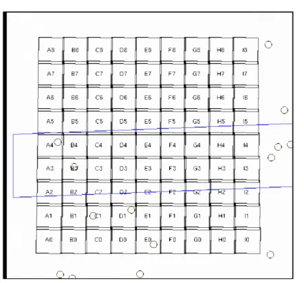
this thesis we have only used data from the primary survey area. If references are made to ‘the survey’ from here on, we implicitly mean the primary survey. The location of the various patches on the sky are shown in Figure 2.2. The lay-out of the exposures within the patch CDE2338 is shown in Figure 2.3 as an example. A number of these patches coincide with other surveys, including the Sloan Digital Sky Survey (SDSS) (York et al. 2000) and the WiggleZ Dark Energy Survey (Blake et al. 2008). Combining data from these surveys is ad-vantageous, as it enables science projects that cannot be performed on either of the data sets individually, as we demonstrate in Chapters 3 and 4.

The observations of the survey were performed in three filters (g0, r0andz0). About half of the survey area is observed in thei0-band as part of the Canada-France High-z quasar survey (Willott et al. 2005), and was made available for the RCS2 through a data exchange agreement. Details of the observations in each of these bands can be found in Table 2.2. Note that the depth of ther0 -and z0-band were chosen to detect M∗+ 1 red-sequence cluster galaxies at a redshiftz∼1.

(29)

cos-Figure 2.1: The variation of the pixel size in the MegaCam camera, also known as the camera distortion, induced by slight non-linearities in the camera optics. The colour bar indicates the size of the pixels in arcsec, and their relative size with respect to the mean. The pixel size is largest in the centre of the camera. The lay-out of the individual chips is clearly discernible. The variation is smooth and constant over time; the small jumps in the pattern between the central chips are caused by a lack of stars to trace the relative astrometry. The camera distortion generates a false shear signal, which has been corrected for in the lensing analyses. This image is a product of the THELI pipeline (Erben et al. 2005, 2009).

mic rays is more difficult, especially those that hit galaxies and stars. However, they introduce no bias in the analyses, but only act as a minor source of noise. To quantify the image quality, the variation of the PSF is measured across the field in each exposure. The images of the stars are used for this purpose because they are essentially point sources. For each star, the Full Width Half Maximum (FWHM) is determined, which is the distance from the star’s centre where the flux reaches half of its maximum value. The median stellar FWHM is a measure of the quality of the PSF; the larger it is, the more the observed images of galaxies are smeared out, which causes them to appear rounder. Cor-recting the observed shapes for this smearing becomes increasingly difficult for larger PSF sizes, particularly for small and faint galaxies. Additionally, the depth of the images decreases if the PSF is large, as very faint galaxies are smeared out such that they become buried in the background noise. Weak lens-ing studies therefore require observations with small PSF sizes.

(30)

2.2. RED SEQUENCE CLUSTER SURVEY 2

Figure 2.2: The location of the RCS2 patches on the sky in Cartesian projection, as a function of right ascension and declination. The grey scale denotes the dust maps from Schlegel et al. (1998). The labels indicate the name of the patches. The name-less patch in the centre is the uncompleted patch 1303, for which no photometric catalogues exist because of its non-contiguous nature (image courtesy: David Gilbank).

Table 2.2: Details on the various observing bands of the RCS2 (PI data) Band Area [deg2] texp [sec] mlim(a) Median seeing

g0 740 240 24.4 0.7900

r0 740 480 24.3 0.7100

i0 400 500 23.7 0.5300

z0 740 360 22.8 0.6700

(a) the 5σpoint source limiting magnitude, averaged over all chips

given in Table 2.2. It differs between the observing bands due to the differ-ence of the atmospheric conditions during the observations. The distribution of the FWHMs in ther0-band, the band used for the lensing analysis, is shown in Figure 2.4. The values of the FWHM range from 0.500 to 1.000, and have a median value of 0.7100. This is exceptionally good for a ground-based survey (e.g. compare Table 2.1.)

(31)

Figure 2.3: The location of the 81 exposures in the patch 2338, as a function of right ascension (horizontal axis) and declination (vertical axis). The circles denote the location of bright stars from the Bright Star Catalogue 4, with a magnitude between 4 and 6. The blue box shows the overlap with the SDSS (image courtesy: rcs2.org)

2.3 Data reduction

The basic reduction of the images is performed with Elixir2 _{at the CFHT.}

Elixir consists of a collection of programs that is used for the instant assessment of the image quality of telescope data, and also contains programs to perform the basic image reduction. The goal of this reduction is to remove the instru-mental signature from the data, so that the images can be used for science. This reduction corrects for the positive offset of the detector of the camera, for the dark current (the electrons that are occasionally released in the CCD due to thermal motions instead of photons), for the unequal sensitivity of the pixels in the CCD, and for the presence of fringes, which are caused by thin-film inter-ference effects in the detector. Once this basic reduction has been performed, objects are detected withSExtractor (Bertin & Arnouts 1996). The locations of the detections are compared to the USNO 1.0 star catalogue to calculate the astrometric solution, such that the (x, y)-locations of the pixels can be trans-lated into sky coordinates. Finally, by comparing the observed photon counts of these stars to their known magnitudes, zero points, that is the conversion factor between counts and apparent magnitude, are calculated for each image.

(32)

2.3. DATA REDUCTION

Figure 2.4: The distribution of the FWHM of the stars in the 739r0-band images in the primary survey area of the RCS2. The solid black (dashed red) line shows the distribution for the images observed after (before) the change of the lens configuration.

Using the zero points, we can determine the apparent magnitudes of all detected objects in the image.

We retrieve the Elixir processed images from the Canadian Astronomy Data Centre (CADC) archive3_{. We use the THELI pipeline (Erben et al. 2005,}

2009) to subtract the image backgrounds, create weight maps that we use in the object detection phase, and to identify satellite and asteroid trails. To ob-tain a more accurate astrometric solution, we runSCAMP (Bertin 2006) on the images, which enables us to match our catalogues to other catalogues, including the photometric catalogues from Gilbank et al. (2011), and the spectroscopic catalogues from the SDSS. Additionally, we use the polynomial coefficients from SCAMPthat describe the mapping from image to sky coordinates to calculate the systematic shear that results from the camera distortion, and for which we have to correct.

(33)

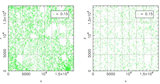
Figure 2.5: The ellipticities of the stars in two exposures as a function of po-sition in the mosaic. The green sticks indicate the size and orientation of the ellipticities of the stars that are used for modeling the PSF (note that only half of the total number of stars is plotted for clarity). The dashed lines approxi-mately denote the chip boundaries. On the left-hand side, we show the stellar ellipticities in the field 2143H6, which was observed before the lens configuration changed. The PSF shows a clear pattern, and is very elliptical in the corners of the image. On the right-hand side, we show the stellar ellipticities in 1613A2, which was observed after the lens-configuration change. No pattern is observed in the PSF, and the PSF ellipticity is small across the image.

Each exposure contains areas where the photometry is affected by the re-flection haloes of large stars, diffraction spikes, satellite and asteroid trails, and other anomalies. Excluding such areas in lensing studies is important, as the shape measurement of galaxies in those areas is unreliable, and may contami-nate the lensing signal. For that purpose, we create image masks for our lensing analyses by combining the masks from the automated masking routines from THELI with the RCS2 masks, as neither of these masks individually works suf-ficiently well for our purposes. The THELI mask poorly covers the large stellar reflections, potentially because we run the pipeline on individual chips. The RCS2 masks covers these large stellar reflections well, but misses many satellite and asteroid trails that are properly masked by THELI. To exclude the contam-inated areas that are not covered by either mask, we inspect all masks by eye, and manually improve them where necessary.

An additional advantage of the visual inspection of the data was the dis-covery of various problematic exposures that were not flagged by the standard image quality checks. Two sets of these exposures are discussed in the last two paragraphs of the next section.

2.3.1 Problematic exposures

(34)

2.4. CATALOGUE CREATION

the science analysis. We describe the problems of these fields below.

During parts of the observing run 05BQ03, the upper half of the camera (chips 18 to 36) was not read out due to a failure in the power supply in the South controller. The four RCS2 r0-band images that were taken in this run have been discarded.

The read-out of chip 5 failed for the twenty-oner0-band exposures taken in observing runs 03BQ06 and 03BQ07. This did not affect the other chips, and the exposures were included.

Ther0-band exposures of the patches 0047F8, 2338I1 and 2338I8 exhibit a strange feature; faint horizontal and vertical trails emerge from the bright stars, which are most likely caused by an electronic problem during the read-out. As it is not clear how this anomaly depends on the brightness, nor whether stars and galaxies are affected in an equivalent way, these three exposures have been removed from the science analyses.

Finally, the central pixels of the bright stars in chip 28 to 36 in the observing runs 04BQ02 and 04BQ03 have negative values. This problem was caused by a failure of the video board in the South controller, which resulted in the ampli-fier saturating at 32K instead of the usual 65K. All the problematic stars are masked, as to make sure they are not used to model the PSF. The exposures have been included in the science analyses.

2.4 Catalogue creation

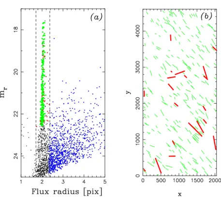
We useSExtractor (Bertin & Arnouts 1996) to detect the objects in the images. From the object catalogues we select the stars, which are used for modeling the PSF variation across the images. An accurate model of the local size and shape of the PSF is essential, as the measured galaxy images have to be corrected for the smearing of the PSF to obtain their unconvolved shapes. Hence we require a clean star catalogue, that contains many stars distributed over the entire image in order to sample the spatial variation of the PSF. To separate the stars from the galaxies, we first identify the locus of the stellar branch in a size-magnitude diagram. We select the non-saturated objects close to the stellar branch with a S/N ratio larger than 30 and with no SExtractor flags raised. To remove small galaxies that have been misidentified as stars, and stars that have been affected by cosmic rays, we fit a second-order polynomial to both the size and the ellipticity of these star-candidates as a function of their position in the chip, and discard all 3-sigma outliers. We clean the stellar selection even further in the shape measurement pipeline by removing shape parameter outliers. All objects larger than 1.2 times the local size of the PSF are classified as galaxies, and passed on to the shape measurement pipeline. Smaller objects are not included as they consist of a mixture of stars and galaxies. The resulting effective galaxy number density is 11.6 arcmin−2_{. Two diagnostic plots of the}

(35)

Figure 2.6: In panel (a), we show the size-magnitude diagram of one of the chips in a randomly picked exposure. The black dots are theSExtractordetections, the green pentagons are the selected stars, the red triangles are the 3-sigma outliers, and the blue squares are the selected galaxies. The dashed lines indicate the location of the stellar branch. Thanks to the good image quality the stars are easily separated from the galaxies. In panel (b), we show the location of the same stars and their ellipticity vectors as a function of position in the chip. The 3-sigma outliers are indicated by the thick red lines.

Elixir provides approximate zero-points for each pointing, which we use to measure ther0-band apparent magnitudes of the objects in the images. We correct the magnitudes for galactic extinction using the dust maps from Schlegel et al. (1998). We asses the quality of the photometry in Section 2.5.

2.4.1 Weak lensing analysis

For our lensing analysis we measure the shapes of galaxies with the KSB method (Kaiser et al. 1995; Luppino & Kaiser 1997; Hoekstra et al. 1998), using the implementation described by Hoekstra et al. (1998, 2000). There are several alternative methods to measure shapes of galaxies. We use the KSB method because it measures the shapes of galaxies accurately in simulations (see Section 2.5), and because it has been extensively used and tested on real data. Finally, the method is fast.

(36)

2.4. CATALOGUE CREATION

call polarizations from here on:

1=

Q11−Q22

Q11+Q22

;2=

Q12

Q11+Q22

, (2.1)

whereQij is the weighted moment of the brightness distribution B(x):

Qij =

Z

d2xB(x)W(x)xixj, (2.2)

with W(x) a Gaussian weight function. The weight function and the integral are centered at the galaxy. To convert the measured galaxy polarizations into ellipticities, the polarizations have to be corrected for the circularization by the weight function, and for smearing by the PSF. These corrections are described by complex formula that can be found in the original papers. To correct for the PSF, we need to determine the smear susceptibility tensor,Psm?_{, which}

de-scribes how the PSF affects the galaxy polarizations. Psm? _{is estimated by the}

combination of various higher-order moments of the brightness distribution of the stars in a chip. The components of the tensor are interpolated at the loca-tion of the galaxies using a polynomial that is third-order iny and second-order in x(the length of the chip in they-direction is more than twice the length in thex-direction), fitted to each chip separately.

The PSF correction has a limited accuracy in practice. One of the reasons is that in the KSB formalism, it is assumed that the brightness distribution of stars can be described by an isotropic profile convolved with a small anisotropic kernel. The PSF is generally more complicated which may lead to biases. To study the magnitude of these biases, this implementation of KSB has been tested on simulations with a variety of PSFs, which we will discuss in Section 2.5.2.

The ellipticities of the galaxies are also affected by slight non-linearities in the mapping between the sky coordinates and the CCD pixels in the camera, an effect which is called camera distortion. We calculate the shear induced by this distortion using the polynomial coefficients fromSCAMP that describe how the image coordinates are mapped onto the sky coordinates. The camera shear of MegaCam is shown in Figure 2.7. The images of both the stars and the galaxies are sheared, with a value reaching 1.5% at the corners of the images. At large lens-source separations, where the gravitational lensing signal is small, the camera shear dominates the observed lensing signal. Hoekstra et al. (1998, 2000) demonstrate that the observed shear is the sum of the gravitational shear and the camera shear. We therefore simply subtract the camera shear from the observed ellipticities of the galaxies to correct for it, after correcting the galaxy shapes for smearing by the PSF.

(37)

Figure 2.7: Shear induced by camera distortion in the MegaCam imager. The camera shear is largest in the corners of the mosaic, with values up to 1.5%. As the observed shear is the sum of the gravitational shear and the camera shear, we simply subtract the camera shear from the observed galaxy ellipticities to correct for it.

the studies of this thesis. Hence the source galaxies at large separations always reside in the corners. Consequently, there is systematic contribution to the real shear. To remove this signal, we measure the lensing signal around a catalogue of random lens positions. In the absence of systematic shear in the shape cata-logues, the shear signal around random lenses is zero, but if systematic shear is present, the random signal and the real signal are equally affected. We use 40 000 random lenses per image, roughly 20 times the number of real lenses used at most per image in the science analyses. The random lensing signal is measured using the same binning, and subtracted from the real lensing signal. We test the correction in the next section.

2.5 Quality Checks

(38)

2.5. QUALITY CHECKS

Figure 2.8: Internal comparison of the r0-band magnitudes of galaxies that reside in the areas that overlap with neighbouring exposures. Each overlapping exposure is indicated by a different colour, and their names shown in the top-left corners. The photometry of the majority of exposures agrees well internally, as the histograms are centered on zero and have a small width. Only a few exposures have erroneous zero-points. We show one example in the right-hand panel, where the zero-point of the image 704853 is off by∼0.5 magnitude.

2.5.1 Photometry

As a check of internal consistency, we compare the magnitudes of the galax-ies from different exposures that reside in the overlapping areas. Depending on its location in the patch, an exposure may overlap with up to 8 neighbours. We match the galaxies from adjacent fields, and make histograms of the difference in

r0-band magnitudes. A few examples are shown in Figure 2.8. These histograms show that for nearly all exposures, the zero-points between neighbouring fields are consistent as the histograms are centered close to zero. Only for a few expo-sures, the histograms are significantly shifted from zero, which indicates that in either one of the exposures the zero-point is far off. As the exposures generally overlap with more than one neighbour, the fields with erroneous photometry are easily identified.

Next, we compare the ‘raw’ dust-correctedr0-band magnitudes of the galax-ies to the more accurately calibrated ones from Gilbank et al. (2011). For each exposure we make a histogram of the difference in magnitudes. A few examples are shown in Figure 2.9. The histograms demonstrate that the magnitudes agree well for the majority of galaxies. The fields with an erroneous zero-point as re-vealed by the internal comparison are easily identified from these histograms as well since they are significantly shifted from 0. None of the histograms are Gaussian, but they all show a tail at mr0−mr0,Gilbank <0. This is likely due

to the fact that different apertures have been used in the measurements. In one exposure, the histograms are offset by ∆mr≈2, indicating that a major error occurred in one of the photometric solutions. On average, however, the magni-tudes agree well, and differ in ther0-band byhmr0−mr0,Gilbanki= 0.00±0.26.

(39)

Figure 2.9: Comparison of ther0-band magnitudes of galaxies with the photo-metric catalogues from Gilbank et al. (2011) for three exposures. The left-hand and middle panel show the same exposures as in Figure 2.8, the right-hand panel shows the exposure with image number 704583 whose zero-point was found to be off, which is again confirmed. The top-left corner of each plot shows the ob-serving run number, the image name, the patch name, the number of galaxies, the percentage of matched galaxies and the mean offset. For the majority of ex-posures, the magnitudes agree well. The non-Gaussian shapes of the histograms are likely due to a difference in the size of the aperture used for measuring the flux.

galaxies withmr0 <23, we findhmr0−mr0,Gilbanki= 0.01±0.14.

In the whole thesis we use the photometric catalogue from Gilbank et al. (2011), except in Chapter 3, as the photometric catalogue was not available at the time of writing. However, in Chapter 3 the ‘raw’ Elixir magnitudes are only used to select the source galaxy sample and for this purpose they are sufficiently accurate.

2.5.2 Galaxy shapes

The implementation of the KSB method we use has been tested on the Shear Testing Programme (STEP) simulations (the HH method in Heymans et al. 2006; Massey et al. 2007). The STEP simulations are used for the blind testing and comparison of shape measurement methods. These simulations con-sist of an artificial set of survey images, containing a large number of galaxies whose morphologies mimic those of real galaxies. To these galaxies a shear is applied which is constant, but differs from image to image. The images are then convolved with a variety of PSFs, to test the reliability of methods under differ-ent observing conditions. The goal of any of the tested methods is to determine as accurately as possible the value of the input shear. Its values is not known beforehand to avoid tweaking of the methods. The performance of each method is determined by two numbers,mi andci, the multiplicative bias and the shear calibration bias, defined as