Advance Access publication 2017 December 15
The very faint X-ray binary IGR J17062-6143: a truncated disc, no
pulsations, and a possible outflow
J. van den Eijnden,
1,2‹N. Degenaar,
1,2C. Pinto,
2A. Patruno,
3,4K. Wette,
5C. Messenger,
6J. V. Hern´andez Santisteban,
1,2R. Wijnands,
1J. M. Miller,
7D. Altamirano,
8F. Paerels,
9,10D. Chakrabarty
11and A. C. Fabian
21Anton Pannekoek Institute for Astronomy, University of Amsterdam, Science Park 904, NL-1098 XH Amsterdam, the Netherlands 2Institute of Astronomy, University of Cambridge, Madingley Road, Cambridge CB3 0HA, UK
3Leiden Observatory, Leiden University, PO Box 9513, NL-2300 RA Leiden, the Netherlands
4ASTRON, The Netherlands Institute for Radio Astronomy, Postbus 2, NL-7990 AA Dwingeloo, the Netherlands 5Albert-Einstein-Institut, Max-Planck-Institut f¨ur Gravitationsphysik, D-30167 Hannover, Germany
6SUPA, School of Physics and Astronomy, University of Glasgow, Glasgow G12 8QQ, UK 7Department of Astronomy, University of Michigan, 500 Church Street, Ann Arbor, MI 48109, USA 8Department of Physics and Astronomy, University of Southampton, Southampton, Hampshire SO171BJ, UK 9Columbia University, Mail Code 5246, 550 West 120th Street, New York, NY 10027, USA
10Columbia Astrophysics Laboratory, Mail Code 5247, 550 West 120th Street, New York, NY 10027, USA
11Massachusetts Institute of Technology (MIT), Kavli Institute for Astrophysics and Space Research, Cambridge, MA 02139, USA
Accepted 2017 December 9. Received 2017 December 9; in original form 2017 August 10
A B S T R A C T
We present a comprehensive X-ray study of the neutron star low-mass X-ray binary IGR J17062-6143, which has been accreting at low luminosities since its discovery in 2006. Analysing NuSTAR, XMM–Newton, and Swift observations, we investigate the very faint nature of this source through three approaches: modelling the relativistic reflection spectrum to constrain the accretion geometry, performing high-resolution X-ray spectroscopy to search for an outflow, and searching for the recently reported millisecond X-ray pulsations. We find a strongly truncated accretion disc at 77+−2218gravitational radii (∼164 km) assuming a high incli-nation, although a low inclination and a disc extending to the neutron star cannot be excluded. The high-resolution spectroscopy reveals evidence for oxygen-rich circumbinary material, possibly resulting from a blueshifted, collisionally ionized outflow. Finally, we do not detect any pulsations. We discuss these results in the broader context of possible explanations for the persistent faint nature of weakly accreting neutron stars. The results are consistent with both an ultra-compact binary orbit and a magnetically truncated accretion flow, although both cannot be unambiguously inferred. We also discuss the nature of the donor star and conclude that it is likely a CO or O–Ne–Mg white dwarf, consistent with recent multiwavelength modelling.
Key words: accretion, accretion discs – stars: neutron – X-rays: binaries – X-rays: individual: IGR J17062-6143.
1 I N T R O D U C T I O N
In low-mass X-ray binaries (LMXBs), either a neutron star (NS) or a black hole (BH) accretes matter from a low-mass companion star overflowing its Roche lobe. Such LMXBs typically are tran-sient systems, displaying outbursts lasting weeks to months and afterwards returning to quiescence for months to years. Around the peak of these outbursts, where the accretion rate typically reaches few tens of per cents of the Eddington rate, the accretion flow is
E-mail:[email protected]
well described by a geometrically thin, optically thick accretion disc extending to the compact object. At lower accretion rates, an addi-tional, poorly understood Comptonizing structure of hot electrons, the corona, is typically located close to the compact object (see
e.g. Done, Gierlinski & Kubota2007; Gilfanov2010, for reviews).
At such lower accretion rates, the accretion flow also changes its
structure significantly (Wagner et al.1994; Campana et al.1997;
Rutledge et al.2002; Kuulkers et al.2009; Bernardini et al.2013;
Cackett et al.2013; Chakrabarty et al.2014; D’Angelo et al.2015;
Rana et al.2016): the inner flow is predicted to transition into a
radiatively inefficient accretion flow (RIAF) as the thin disc
evap-orates into a hot, thick flow (Narayan & Yi1994; Blandford &
2017 The Author(s)
Padilla, Wijnands & Degenaar2013b; Armas Padilla et al.2013a;
Degenaar et al.2013; Wijnands et al.2015). Finally, the magnetic
field of the NS can interact with the accretion flow, possibly trun-cating the disc away from the compact object (e.g. Illarionov &
Sunyaev1975; Cackett et al.2010; D’Angelo & Spruit2010). As
the gas pressure decreases towards lower accretion rates, this in-teraction and truncation might be more efficient in this accretion regime. Disc truncations have been inferred in a few NS LMXBs at larger radii than in BHs at similar accretion rates, possible
in-deed caused by the NS magnetic fields (e.g. Tomsick et al.2009;
Degenaar et al.2014; F¨urst et al.2016; Iaria et al.2016; Degenaar
et al.2017a; Ludlam et al.2017b; van den Eijnden et al.2017, see
the Appendix for a detailed comparison.).
The low-luminosity epochs during the outbursts decays in tran-sient LMXBs are challenging to study due to the short time-scales and low fluxes involved. However, interestingly, a small sample of NS LMXBs is observed to accrete in this transition regime
persis-tently for years (LX∼10−4–10−2LEdd, whereLEddis the Eddington
luminosity, corresponding to the maximum possible accretion rate
Chelovekov & Grebenev 2007; Del Santo et al. 2007; Jonker &
Keek2008; Heinke, Cohn & Lugger2009; in’t Zand et al.2009;
Degenaar et al.2010,2017a; Armas Padilla et al.2013b). These
sources, called very faint X-ray binaries (VFXBs), are thus interest-ing to study the low-level accretion regime in between outburst and quiescence. However, these sources evidently have an additional complication: it is currently unclear how they can persistently ac-crete at such low levels, and this persistent nature might make their faint properties different from transient sources.
Two different explanations have been proposed to account for the persistently faint nature of VFXBs: magnetic inhibition of the accretion flow and an ultra-compact nature of the binary. In the for-mer, a strong NS magnetic field truncates the inner accretion disc,
effectively preventing efficient accretion (Degenaar et al. 2014,
2017a; Heinke et al.2015). In this scenario, the field lines might act as a magnetic propeller, which could cause the expulsion of gas into an outflow and reduces the accretion efficiency. Alternatively, only a small accretion disc physically fits into the compact binary orbit of a so-called ultra-compact X-ray binary (UCXB; King &
Wijnands 2006; in’t Zand, Jonker & Markwardt2007; Hameury
& Lasota2016). The second scenario can evidently be tested
di-rectly by measuring the orbital parameters. More indidi-rectly, as the small orbit does not fit a hydrogen-rich donor (e.g. Nelemans et al.
2004; in’t Zand et al.2009), a lack of hydrogen emission from the
accretion disc can hint towards an ultra-compact orbit. However, several LMXBs lacking hydrogen emission without having an ultra-compact orbit have been detected, and additionally, a VFXB with
et al. (2017a, hereafterD17), analysing simultaneousSwift,
Chan-dra,andNuSTARobservations. TheNuSTARandChandraspectra clearly revealed a broad iron-K line around 6.5 keV, for the first time
at such a low (2.5×10⁻³LEdd) accretion rate in an NS LMXB. This
iron-K line is the most prominent feature of the reflection spectrum: photons originating from close to the compact object (for instance from the Comptonizing hot flow) reflecting off the disc into our line of sight. The iron-K line profile feature is altered into a broad-ened shape by the rotation of the disc, gravitational redshift, and
relativistic boosting (Fabian et al.1989). Hence, by modelling both
this line and the remainder of the reflection spectrum, it is possible to infer geometrical parameters such as the inner disc radius and inclination of the system.
Through detailed modelling of the reflection spectrum,D17
in-ferred that the accretion disc is truncated far from the NS atRin
100Rg, whereRg=GM/c2is the gravitational radius (∼2.07 km for
a 1.4 MNS). Although the innermost stable circular orbit (ISCO;
6Rgfor a non-spinning compact object) could not be excluded at
3σ, this inferred inner radius is significantly larger than typically
observed in accreting NSs. At these low accretion rates, it is difficult to definitively distinguish between the NS’s magnetic field truncat-ing the disc, or the formation of a hot inner flow resulttruncat-ing in a large inner disc radius. However, for J1706, the inferred inner radius is also significantly larger than observed in two BH LMXBs at similar
or lower accretion rates:≥35Rgin GX 339-4 (Tomsick et al.2009)
and 12–35Rgin GRS 1739-278 (F¨urst et al.2016). As the formation
of a hot flow might also be more efficient in BHs, due to the lack of photons from the NS surface cooling the flow (e.g. Narayan & Yi
1995),D17concluded that the disc in J1706 is likely truncated by
the magnetic field. Under that assumption, the measured flux and
Rinpredict a magnetic field ofB4×108G.
Additionally,D17performed high-resolution X-ray spectroscopy
on the Chandra-HETG spectra. Several (marginally) significant
emission and absorption lines could be detected, although an unam-biguous identification was not possible. The presence of blueshifted absorption suggests the presence of a wind, which might be driven by a propeller resulting from the magnetic truncation of the disc or alternatively radiation pressure in the disc. Interestingly, if the outflow is propeller-driven, combined with the possible magnetic truncation of the accretion disc, this appears to be consistent with the idea of magnetic inhibition in VFXBs introduced above. How-ever, due to the low flux of J1706, both results are merely marginally significant and require independent confirmation with new observa-tions. The recent detection of 163 Hz coherent X-ray pulsations in
J1706 by Strohmayer & Keek (2017) is consistent with this picture
However, evidence for an ultra-compact nature of J1706 was
also recently found. Hern´andez Santisteban et al. (2017) performed
a multiwavelength study covering the optical, UV and NIR. Optical Geminispectroscopy revealed a blue but featureless disc spectrum, consistent with a hydrogen-poor donor star, as is expected in UCXBs
(in’t Zand et al.2009). In addition, the modelling of the complete
disc spectral-energy distribution (SED) provides an estimate of the orbital period of 0.6–1.3 h. Hence, arguments can be made both for an ultra-compact nature and for magnetic inhibition of the accretion flow in J1706, and new, detailed observational studies are required to fully understand its persistently low accretion rate.
In this paper, we present a detailed study of new and archival
X-ray observations of J1706 byNuSTAR,XMM–Newton,andSwift,
aiming to understand its VFXB nature through three approaches:
high-resolution X-ray spectroscopy of theXMM–NewtonRGS
spec-tra, broad-band reflection modelling of all observations, and finally
an extensive pulsation search in theXMM–NewtonEPIC-pn data.
While the low flux of VFXBs makes each of these individual meth-ods challenging, their combination yields firmer constraints on the accretion properties of J1706.
2 O B S E RVAT I O N S
We extended the set of observations of J1706 analysed byD17,
which consisted ofNuSTAR, Swift(both from 2015) and
Chan-dra(from 2014) observations, with new, simultaneousNuSTARand
XMM–Newtonobservations from September 2016. For the 2015 observations, we applied the same approach to the data reduction as
D17. For clarity, we briefly review that approach in this section, in
addition to a more detailed discussion of the 2016 data. During the
2016 observations, J1706 shows a∼16 per cent lower luminosity
than in the 2015 data; we will discuss the similarities and discrep-ancies between the two data sets in Section 3. We included the 2015 Swiftobservation to increase the soft spectral coverage during the
2015 epoch. We did not reanalyse theChandra-observation, but
in-stead focused onXMM–NewtonRGS in our search for narrow line
features. During none of the analysed observation a Type-I burst was observed.
2.1 NuSTAR
NuSTAR(Harrison et al.2013) observed J1706 from 2015 19:26:07 May 6 to 05:01:07 May 8 (ObsId 30101034002) and from 2016 08:46:08 September 13 to 14:36:08 September 14 (ObsId
30101018002). We applied the standardNUPIPELINEandNUPRODUCTS
software to extract source and background spectra, and light curves, for both observations. The 2015 and 2016 observations amount to a
∼70 and∼67 ks exposure, respectively. FollowingD17, we selected
a 30 arcsec circular source region and a 60 arcsec background
re-gion from the same chip in both observations. As inD17, we found
a negligible (<0.5 per cent) difference in normalization between
the Focal Plane Module A and B (FPMA/FPMB) spectra in the 2015 observation; hence, we combined the data from the two
mod-ules usingADDASCASPECandADDRMF. The 2016 observation shows
larger deviations between FPMA and FPMB (∼6 per cent), and are
thus not combined but rather fitted simultaneously with a constant floating in between. Finally, we rebinned the combined 2015 spec-trum and two separate 2016 FPMA and FPMB spectra to contain at least 20 counts per bin. J1706 is detected above the background in the entire 3–79 keV bandpass in the 2015 observation, and in the 3–50 keV range in the 2016 data.
2.2 Swift
The Swift (Gehrels et al. 2004) X-ray Telescope (XRT) ob-served J1706 in Photon Counting mode on 2015 May 6 (ObsId
00037808005), simultaneously with the firstNuSTARobservation,
amounting to a∼0.9 ks exposure. We again followed the extraction
approach inD17. UsingXSELECT, we extracted a source spectrum
from a 12 to 71 arcsec annulus to circumvent pile-up issues, and a background spectrum from a void region three times the size. We
produced an arf file withXRTMKARFand used the appropriate rmf file
(version 15:SWXWT0TO2S6_20131212V015.RMF) from theCALDB.
Fi-nally, we rebinned the spectrum to contain a minimum of 20 counts per bin.
2.3 XMM–Newton
XMM–Newton (Jansen et al. 2001) observed J1706 from 2016 12:21:18 September 13 to 06:04:51 September 15 (ObsId 0790780101). We extracted spectra from the EPIC-pn, which
op-erated in timing mode, and RGS detectors using theXMM–Newton
SASv15 following the standard procedures in theSAScookbook.1
The EPIC-pn 10-12 keV light curve does not show any background flaring, so we used all available data. We extracted the EPIC-pn source and background spectra from regions of RAWX between 30
and 46, and between 2 and 6, respectively. Using theFTOOL EPAT
-PLOT, we explicitly checked for pile-up in the spectrum, which is
not present. We extracted the RGS spectra following the standard
SASguidelines, combining the two detectors into one spectrum per
order after visually confirming that the two detectors are consistent. We analyse the resulting RGS first- and second-order spectra in the 7.0–28.0 and 7.0–16.0 Å wavelength ranges, respectively.
3 B R OA D - B A N D S P E C T R A L A N A LY S I S
We fitted the X-ray spectra usingXSPEC v12.9.0 (Arnaud1996).
In order to model the interstellar absorption, we included either TBABSorTBNEWin each model, depending on whether we use Solar abundances in the absorption column. We used cross-sections from
Verner et al. (1996) and Solar abundances from Wilms, Allen &
McCray (2000). In addition, we included a floating constant
be-tween all spectra to account for normalization offsets bebe-tween the
data sets. We quote uncertainties at the 1σlevel.
3.1 Phenomenological modelling
D17 phenomenologically described the 2015 Swiftand NuSTAR
spectra with a model consisting of a power law (PEGPWRLW) and a
blackbody (BBODYRAD). To investigate the similarity between the
spectra from the 2015 and 2016 observations, we first applied the same model to the 2016 data only – note that we did not include the RGS spectrum in this broad-band modelling, but in-stead separately focus on it in Section 4. Due to the increased
quality of theXMM–NewtonEPIC-pn spectrum compared to the
Swiftspectrum, this phenomenological model does not provide an
adequate description below 3 keV [χ2
ν ∼2.9 for 849 degrees of
freedom (dof)]. Large residuals remain around 1 keV, which cannot
be described by an additionalDISKBBcomponent representing the
accretion disc (χ2
ν ∼2.7). Instead including an additional
Gaus-sian component at this energy resulted in a highly improved fit
1https://heasarc.gsfc.nasa.gov/docs/xmm/abc/
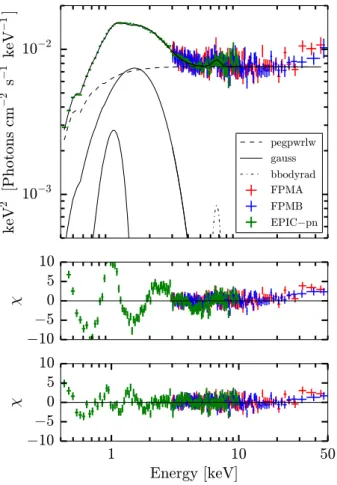
Figure 1. Top: The 2016 XMM–Newton EPIC-pn (green) and NuSTAR FPMA (red) and FPMB (blue) spectra unfolded around the best-fitting phenomenological model CONSTANT*TBABS* (BBODYRAD+PEGPWRLW+GAUSS+GAUSS). The FPMB and EPIC-pn spectra have been rescaled by their fitted cross-calibration constant for visual clarity. Middle:χfor the phenomenological model inD17, showing a broad Fe Kαfeature and an emission feature around∼1 keV. Bottom:χ for the best-fitting phenomenological model. We discuss the residuals remaining below 2 keV in detail in Section 4.
(χ2
ν =1083.8/846=1.28), with the Gaussian centroid energy and
width equal to 0.96±0.01 keV and 0.18±0.01 keV, respectively
(see Section 4 for a detailed analysis of this feature). The
power-law index equals=2.00±0.01, while the blackbody
tempera-ture and radius areTBB=0.365±0.003 keV andRBB=(6.96±
0.2)[D/7.3kpc] km, respectively. Interestingly, this blackbody
tem-perature is significantly lower than theTBB=0.46±0.03 keV found
byD17.
In Fig.1, we show the unfolded 2016 spectra in the upper panel,
and the residuals for theD17-phenomenological model in the
mid-dle panel. The 2015 observations of J1706 contain a significant Fe
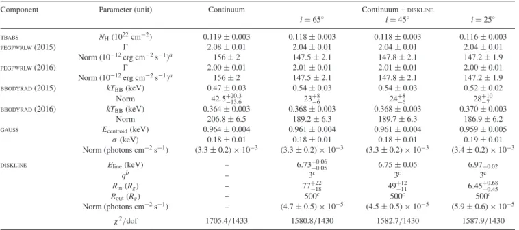
Kαline; zooming in on the residuals of the 2016 data fitted to the
continuum model (see Fig.2), suggests the presence of a similar
broad feature. To test whether this broad line is significant in the 2016 data as well, we added a Gaussian line to the phenomeno-logical model with a centroid energy constrained to 6.4–6.97 keV
(the possible range for Fe Kαemission). This results in a better
fit, withχ2
ν =1020.32/843=1.21 (f-test rejection probability of
5×10⁻¹¹) and a line normalization of (2.2±0.35)×10−5photons
cm−2s−1. The resulting Gaussian parameters are a centroid energy
of 6.65 ± 0.08 keV, a width of 0.47+0.09
−0.08keV, and an equivalent
Figure 2. Data-to-model ratio of the 2016XMM–NewtonEPIC-pn (black) andNuSTARFPMA (red) spectra fitted with a simple continuum model (see Section 3.1). An excess emission feature around the Fe Kαenergy (6.4–6.97 keV) is clearly visible. The spectrum has been rebinned for visual purposes.
width of EW=120 eV, all within the typical range for Gaussian
iron lines (e.g. Ng et al.2010).
The bottom panel in Fig.1shows the residuals after the inclusion
of the two Gaussian features at∼1.0 keV and∼6.66 keV. Some
residuals below 2 keV remain after the inclusion of a Gaussian around 1 keV; we will investigate the nature of these residuals in detail in Section 4. Finally, slightly positive residuals are present
above∼30 keV. However, the inclusion of a second power-law
com-ponent (as inD17) does not significantly improve the fit (p=0.01
for an unphysical power-law index of= −2.5). Refitting the
con-tinuum model up to 30 keV only does not result in any changes in the parameters, so these residuals do not influence the fit. We also
note that an absorption feature appears to be present at∼8.2 keV.
However, as this feature is only present in the EPIC-pn spectrum
(see e.g. Fig.2), it most probably originates from known Ni, Cu,
and Zn fluorescence lines in the internal instrument background
spectrum around this energy.2
Extending the best-fitting phenomenological model to the 0.3–
79 keV range yields an unabsorbed flux of (0.98 ± 0.02) ×
10−10erg s−1cm−2, which is only slightly lower than the flux during
the 2015 observations ((1.17±0.02)×10−10erg s−1cm−2). Given
this similarity in flux, spectral shape and parameters (apart from the
∼1 keV excess), and the presence of a Fe Kαline, we subsequently
fitted the 2015 and 2016 observations together.
3.2 Relativistic reflection models
3.2.1 The iron line:DISKLINE
Before including relativistic reflection in our spectral model, we first analysed the continuum in the 2015 and 2016 observations
to-gether. Simply applying a model consisting ofPEGPWRLW,BBODYRAD
and a Gaussian around 1 keV with all parameters tied results in
a bad fit, withχ2
ν =1905.3/1436=1.33. This is not surprising
given the difference in flux, and so we check which parameters dif-fer significantly between the two epochs. Inspection of the residuals
Table 1. Best-fitting parameters to theNuSTARcombined FPMA&B (2015),Swift-XRT(2015),FPMA AND FPMB(2016),ANDXMM–NewtonEPIC-pn (2016) spectra. For parameters unlinked between the 2015 and 2016 data sets, the year is noted with the model component. The continuum model does not contain any Fe Kαcomponent.
Component Parameter (unit) Continuum Continuum +DISKLINE
i=65◦ i=45◦ i=25◦
TBABS NH(1022cm−2) 0.119±0.003 0.118±0.003 0.118±0.003 0.116±0.003
PEGPWRLW(2015) 2.08±0.01 2.04±0.01 2.04±0.01 2.04±0.01
Norm (10−12erg cm−2s−1)a 156±2 147.5±2.1 147.8±2.1 147.2±1.9
PEGPWRLW(2016) 2.00±0.01 2.01±0.01 2.01±0.01 2.00±0.01
Norm (10−12erg cm−2s−1)a 156±2 147.5±2.1 147.8±2.1 147.2±1.9
BBODYRAD(2015) kTBB(keV) 0.47±0.03 0.54±0.03 0.54±0.03 0.52±0.02
Norm 42.5+−2013..36 23−+86 24+−86 28+−107
BBODYRAD(2016) kTBB(keV) 0.364±0.003 0.368±0.003 0.368±0.003 0.370±0.003
Norm 206.8±6.5 189.2±6.3 189.7±6.3 186.9±6.2
GAUSS Ecentroid(keV) 0.964±0.004 0.961±0.004 0.961±0.004 0.959±0.005
σ(keV) 0.18±0.01 0.18±0.01 0.18±0.01 0.19±0.01
Norm (photons cm−2s−1) (3.3±0.2)×10−3 (3.3±0.2)×10−3 (3.3±0.2)×10−3 (3.4±0.2)×10−3
DISKLINE Eline(keV) – 6.73+−00..0605 6.75±0.05 6.97−0.02
qb – 3c 3c 3c
Rin(Rg) – 77+−2218 49+
12
−11 6.45+
0.68
−0.45
Rout(Rg) – 500c 500c 500c
Norm (photons cm−2s−1) – (4.7±0.5)×10−5 (4.5±0.5)×10−5 (5.9±0.6)×10−5
χ2/dof 1705.4/1433 1580.8/1430 1582.7/1430 1587.9/1430
Notes.aFlux between 0.3 and 79 keV;bemissivity index;cfrozen.
reveals clear differences between the two data sets below 3 keV and a possibly different power-law index. Indeed, untying the black-body temperature and radius results in a significantly improved fit
(χ2
ν =1730.0/1434=1.21;f-test rejection probabilityp∼10−31).
In addition, untying the power-law index also results in
a marginally significant improvement (χ2
ν =1705.4/1433=
1.19; p = 6 × 10⁻⁶), with a slightly harder spectrum
in 2016 ( = 2.00 ± 0.01 compared to 2.08 ± 0.01).
Untying the power-law normalization however does not re-sult in a significant improvement of the fit, both when the power-law index is tied between the two epochs or free. All parameters of the final continuum model are listed in
Table1.
We first modelled the Fe Kαline using theDISKLINEmodel (Fabian
et al.1989), which models a single emission line from the accretion
disc, assuming a Schwarzschild metric, e.g. a dimensionless spin
parameter ofa=0.0. For NSs, the spinatypically ranges from
0.0 to 0.3, where it only minimally impacts the surrounding
met-ric. Initially, we do not link theDISKLINEparameters between the
2015 and 2016 observations. As in the 2015 observations alone,
the inclination is ill-constrained in the 2016 observations. Asχ2is
minimum ati≈67–69◦, we followedD17and initially fixed the
inclination to 65◦. The fitted iron line parameters (line energy, inner
disc radius and normalization) are all consistent between the 2015 and 2016 epochs. Hence, to increase the accuracy of our parameter determination, we link all three between the 2015 and 2016 spectra.
The resulting fit (χ2
ν =1580.8/1430=1.11) implies an inner disc
radius ofRin=77+−2218Rg, with the ISCO excluded at a significance
of∼6.2σ.
As we will discuss in Section 6.1.4 in detail, the reflecting disc itself is not observed in the X-rays. It is however clearly observed
in the source’s SED (Hern´andez Santisteban et al.2017). The inner
disc radius measurement from reflection spectroscopy is consistent with the modelling of this SED, as the SED only constrains the inner radius to be larger than the NS radius. Detecting the accretion disc in the SED but not in the X-ray spectrum is consistent with a large
truncation radius, as the accretion disc X-ray emission originates from the innermost regions.
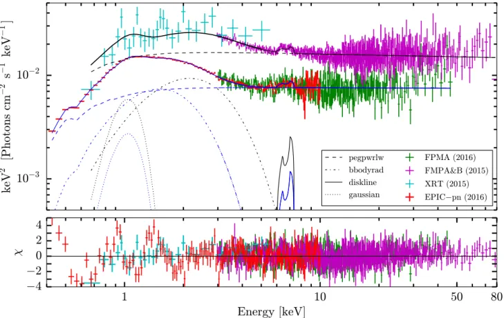
All parameters are listed in Table1, and the unfolded spectrum,
best-fitting model and its residuals are plotted in Fig.3. We note
that theDISKLINEmodel does not provide a better fit to the 2015 and
2016 data simultaneously than a simple Gaussian line. This is not entirely surprising, as the large truncation radius implies a smaller distortion of the iron line shape by relativistic effects.
The bottom panel of Fig.3shows that significant residuals
re-main below 2 keV. As can also be seen in the bottom two panels
of Fig.1, including a Gaussian feature around 1 keV improves the
model fit, but does evidently not describe the feature completely. To test the effect of this residual structure, we have refitted the full model excluding energies below 2 keV. We only find significant
changes in the parameters of theBBODYRADand theGAUSSIAN
com-ponents. This is unsurprising, as the part of the spectrum described by these components is now removed. All other parameters remain unchanged. Interestingly, we also find that excluding the data below
2 keV yields aχ2
ν of 1360.95/1368≈1.00 for the remaining data.
Hence, we are confident that the residuals below 2 keV do not in-fluence our model fit. We will discuss these residuals in more detail in Section 4.
As stated, the inclination of theDISKLINE model is poorly
con-strained: all values between 5◦and 90◦lie within 3σ (e.g.χ2≤
9). Explicitly stepping through a grid in inclination and inner radius
reveals a complicatedχ2space, where a high inclination and a
trun-cated disc minimizesχ2but a second, isolated minimum exists at
an inclination of∼25◦and an inner radius around the ISCO. Hence,
we cannot exclude a disc viewed at low inclination extending to the ISCO. We will discuss this further in Section 6.1.
For clarity, in Table1, we also show the fit parameters for fixed
inclinations of 45◦ (yieldingχ2= +1.85 andR
in=49+−1211 Rg)
and 25◦(yieldingχ2= +7.05,R
in=6.45+−00..6845Rg). In the latter,
the iron line energy sits at its maximum value of 6.97 keV. The con-tinuum parameters do not change significantly with the inclination. Similarly, including the RGS spectrum does not influence either
Figure 3. The best-fitting relativistic-reflection model with theXMM–NewtonEPIC-pn,Swift-XRT, and twoNuSTARobservations. Top: All spectra unfolded around the best-fittingCONSTANT*TBABS*(BBODYRAD+PEGPWRLW+GAUSS+DISKLINE) model. For visual clarity, the two sets of simultaneously observed spectra have separately been rescaled by their fitted cross-calibration constant. For the same reason, we also do not plot the 2016 FPMB spectrum, which is consistent with the FPMA data. See Section 3.2 for details on which parameters were tied between the two observational epochs. Bottom: Residuals of the best-fitting relativistic reflection model. Note that despite the Gaussian component, residual structure remains around∼1 keV, which we investigate in detail in Section 4.
the parameters or the significances quoted in this and the previous paragraphs.
Using theRELXILLreflection model,D17found a similarly
trun-cated accretion disc in the 2015-only data, although the ISCO could
not be excluded at 3σ. When instead modelling the 2015 data with
DISKLINEreflection, we can exclude the ISCO at a significance of
∼4σ. Thus, the addition of the 2016 observations allows us to more
confidently infer that the inner disc in J1706 is truncated away from the ISCO.
3.2.2 Broad-band reflection:RELXILLandREFLIONX
A full relativistic reflection spectrum not only consists of the Fe
Kαline but also contributes to the complete X-ray continuum, for
instance through the presence of a Compton hump peaking around
10–20 keV. Hence, we extended our analysis from theDISKLINE
re-flection model to self-consistent models of the complete relativisti-cally smeared reflection spectrum. We considered two options: (1) RELXILL(Dauser et al.2014; Garc´ıa et al.2014), which models the illuminating power-law component simultaneously with the
reflec-tion and thus replacesPEGPWRLW, and (2)REFLIONX(Ross & Fabian
2005) convolved with theRELCONV-model. In the second option, the
illuminating flux is provided by thePEGPWRLW-component in the
continuum, whose power-law index is thus linked to the reflection
spectrum. In both models, we again fixed the dimensionless spina
to zero, the inclination to 65◦and assume an unbroken emissivity
profile with indexq=3, consistent with both theoretical
predic-tions (Wilkins & Fabian2012) and observations (e.g. Cackett et al.
2010). Finally, we set the iron abundance to one and initially linked
all reflection parameters between the 2015 and 2016 observations.
Note that the untied continuum parameters (in theBLACKBODYand
PEGPWRLW) remained untied.
Both broad-band relativistic reflection models are unable to de-scribe the 2015 and 2016 observations simultaneously with
physi-cally realistic parameters. The first model, usingRELXILL, yields aχ2
ν
of 1670.9/1430=1.17(χ2≈ +90 compared to the best
DISKLINE models for the same number of free parameters). Importantly, the reflection parameters are ill-constrained: the inner radius pegs at the
minimum value of 6Rg, but all values up to 120Rgare consistent
within 3σ. Additionally, the iron line complex is badly modelled:
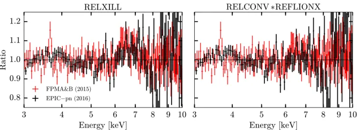
Fig.4(left) shows the residuals between 3 and 10 keV, showing
clear residual iron line structure around 6.5 keV. Similar problems
arise for the second,REFLIONX-based model. While the quality of the
fit is slightly better (χ2
ν =1602.3/1430=1.12), the inner radius
is again unconstrained: its best-fitting value is∼395Rg, while the
outer disc radius was fixed to 400Rg, and all values down to the
ISCO are consistent within 3σ. Furthermore, again clear residual
structure remains in the data-to-model ratio, as can be seen in the
right-hand panel of Fig.4.
Despite the similarities between the 2015 and 2016 spectra, fitting both simultaneously with a broad-band reflection spectrum could be the cause of the problems detailed above. However, untying the reflection parameters between the two sets of observations does not
Figure 4. Data-to-model ratios for theRELXILL(left) andREFLIONX-based (right) broad-band reflection models. The red data in both panels are the combined 2015NuSTARspectrum, while the black data are the 2016XMM–NewtonEPIC-pn spectrum. In both cases, clear iron-line residual structure remains between ∼6 and 7 keV.
significant improvement (χ2≈ −37 for four additional dof,f
-test rejection probability∼2×10⁻⁶), but the inner radii remain
unconstrained and the residual structure does not disappear. For the REFLIONXmodels, untying the reflection parameters does not result
in a significant improvement (χ2≈13 fordof=3,f-test
rejec-tion probabilityp∼0.009), while the two inner radii both exceed
400Rg. Finally, the same iron-line structure in the data-to-model
ra-tio remains. For both models, we also attempted a broken emissivity
profile withq1=0 andq2=3, which is more appropriate for a large
scale height of the corona – again, this offered no improvements to the modelling.
Based on the above considerations, we conclude that the data quality of our 2016 observations is not sufficient to constrain the
full broad-band relativistic reflection spectrum.D17were able to
model the 2015 observation usingRELXILL, although the inferred
inner radius was barely constrained; whileRin was found to
ex-ceed 100Rg, the ISCO could not be excluded. Even though we
fixed several parameters in our reflection fits (amongst others spin and inclination), the lower flux in the 2016 observation does not
allow us to apply a model more complicated thanDISKLINE. It should
be noted again that in 2015, J1706 was the first NS LMXB where the iron line could even be detected at these low fluxes. Hence, it is not surprising that the data do not allow for the most detailed analysis of the reflection.
3.2.3 The∼1keVexcess
Finally, we briefly discuss the∼1 keV excess emission. Similar soft
excesses have been observed in the fast modes of the EPIC-pn
in-strument (XMM-SOC-CAL-TN-00833). However, this
instrumen-tal effect is typically observed in highly obscured sources. AsNH
is a factor of5 lower for J1706 than the sources where this issue
is reported, we do not expect that this effect plays a role (see for
instance Hiemstra et al. (2011), where theNHis∼65 times higher).
As discussed later, we also observe a similar feature in the RGS spectrum, strengthening the case that the feature is real.
Alternatively, it could arise from reflection. In addition to the iron line and the Compton hump, reflection can provide a significant
3http://xmm2.esac.esa.int/external/xmm_sw_cal/calib/documentation/
index.shtml
contribution around 1 keV. As suggested byD17and the failure
of broad-band reflection models to describe the data, the∼1 keV
excess might thus originate from a second, more distant reflection
site. Hence, we adjusted the best-fittingDISKLINEmodel, replacing
the∼1 keV Gaussian component with a second, unlinkedDISKLINE
component. However, this results in a significantly worse fit, with
χ2≈ +320 for the same number of free parameters. Moreover,
the second reflection site would be located at ∼17Rg, which is
within the truncation of the accretion disc inferred from the iron line. Hence, we do not find evidence for a second reflection site from the EPIC-pn data.
4 H I G H - R E S O L U T I O N S P E C T R O S C O P Y
In the 2014Chandra-HETG observation of J1706,D17detected
several marginally significant emission and absorption lines, possi-bly originating from an outflow. However, the unambiguous iden-tification of the lines and their origin proved difficult based on the Chandradata alone. Our XMM–NewtonEPIC-pn spectrum
con-tains a clear excess around 0.9–1.0 keV (∼12–13Å). In order to
investigate the nature of this excess and revisit the detection of the
narrow lines in theChandraspectrum, we perform a high-resolution
spectral analysis of theXMM–NewtonRGS spectrum. In this
sec-tion, we first discuss the RGS continuum, followed by an initial phenomenological line search and subsequent physical modelling. In this section, we switch from energy in keV to wavelength in Å, as is common in high-resolution X-ray spectroscopy.
4.1 RGS continuum
Before focusing on narrow lines and the∼1 keV excess, we
in-vestigated the properties of the RGS continuum. The ∼1 keV
(∼12.4 Å) excess emission in the EPIC-pn spectrum is described
with a simple Gaussian in the previous section, but the bottom panel
of Fig.3shows that this is not fully adequate. Fig.5(top panel)
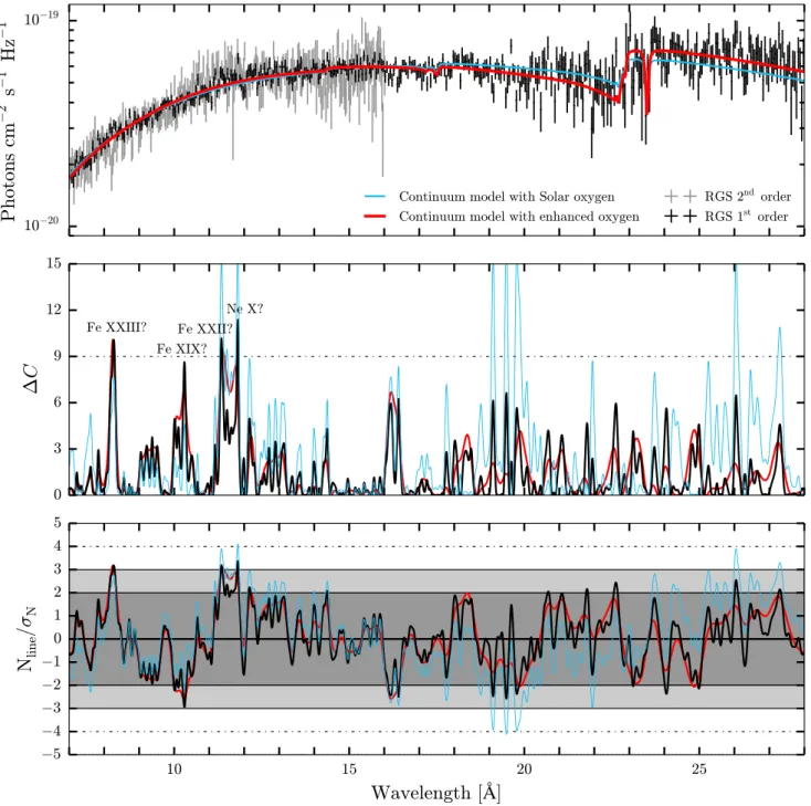
shows the first- and second-order RGS spectra, unfolded around a constant. An emission excess is visible around 11–12 Å, together with a strong oxygen edge around 23 Å. The neon edge around 14.2 Å, though, appears not as strong as the oxygen edge. In a number of bins, the first- and second-order spectra deviate more
Figure 5. Results of the narrow line search in the RGS spectra for two different continuum models. The top panel shows the RGS spectra and the two continuum models, all unfolded around a constant to remove the instrument response. The middle panel shows the improvement in C-statistic for the addition of one free parameter (the line normalization). The dashed line indicatesC=9, corresponding to a 3σsingle-trial significance. The bottom panel shows the fitted line normalization divided by its 1σuncertainty, where a positive normalization implies emission and a negative one absorption. Different colours correspond to different continua: the black and red curves are calculated with theTBNEW*(BBODYRAD+PO) model, assuming free O and, respectively, a 500 and 2000 km s−1line width. The blue curve corresponds to a model with Solar abundances in the absorption column; the remaining trends inN
line/σNreveal the need for a non-Solar oxygen abundances.
than the uncertainties and hence the results of more detailed line modelling (Section 4.3) should be interpreted with caution.
We first attempted to describe the RGS continuum with a sim-ple absorbed blackbody model. However, such a model does not provide a good description of the data; the first-order spectrum is ill described around and above the oxygen edge. Although the
blackbody temperature of TBB ≈ 0.35 keV is consistent with the
broad-band spectral analysis, the hydrogen column density NH
≈ 0.35 ×1021cm−2 is a factor of 3 below typically observed
values and predictions based on Interstellar Medium (ISM) maps
(Kalberla et al. 2005). Including a POWERLAW component, with
fixed to a value of 2.05 since it is ill constrained at these
low energies, significantly improves the continuum description: χ2
ν =946.30/768=1.23 (f-test rejection probabilityp∼10−13).
While the resultingNH≈1.2×1021cm−2andTBB≈0.33 keV are
in line with the full spectrum, the discrepancies around and above
the oxygen edge largely remain (see the blue model in Fig.5, top
To more accurately model the oxygen edge in the continuum, we
replaced the simple absorption modelTBABSby the more detailed
TBNEWmodel. TheTBNEWmodel allows the absorption abundances of individual species to vary with respect to the Solar abundances
by Wilms et al. (2000). We fixed the value ofNHto 1.2×1021cm−2
(Kalberla et al.2005) and first allowed oxygen to vary. This model
results in a significantly improved fit of the first- and second-order
RGS spectra (χ2
ν =856.36/767=1.12,f-test rejection probability
p∼10−18) for a high oxygen abundance ofAO=1.94, and a
black-body temperature ofTBB≈0.31 keV. Fig.5shows this continuum
model both with solar abundances and an enhanced oxygen abun-dance; the discrepancies between the two models above 18 Å are evident. Alternatively, instead of being due to a an enhanced oxy-gen abundance, the excess emission above the oxyoxy-gen edge might result from a combination of many C and N lines. However, such lines are clearly not resolved and an enhanced oxygen abundance is sufficient to model to full continuum.
In order to understand the nature of the high oxygen abundance, we also attempted to free the magnesium, iron, and neon abundances for both a fixed and a free oxygen abundance. None of these options resulted in a significant improvement of the fit. It appears that, with the exception of oxygen, all absorption edges are correctly modelled by the (fixed) interstellar value of the hydrogen absorption. This implies that the high oxygen abundance originates from the source – if it were interstellar, a similar increase would be expected for other abundances, such as neon. Secondly, the oxygen abundance in the ISM is not expected to deviate from the solar value by more
than a factor of ∼1.3 (Pinto et al. 2013). Hence, the additional
oxygen absorption might instead have a circumbinary origin, as we will discuss in Section 6.1.1.
4.2 Line search
After analysing the continuum properties in the RGS spectra, we turned to an explorative search for narrow emission and absorption lines. Following the method detailed in Pinto, Middleton & Fabian
(2016), we adopted the continuum model and subsequently added
a narrow Gaussian line with a fixed width of 500 or 2000 km s−1.
We then fitted the normalization of this Gaussian line, calculated its error, shifted the line by 0.01 Å and repeated. This procedure returns, at each grid point in wavelength, two indications for the presence of a narrow line: the line normalization divided by its error and
the improvement in theC-statisticC. Note that we employ the
C-statistic instead ofχ2-statistics for the detailed line search and
the subsequent line modelling, as it is more accurate for low counts
per bin. We stress that both measures aresingle trialestimations of
the significance of the narrow line; both merely hint to the presence of emission or absorption but can be prone to false positives when considering only a single data set. Hence, the comparison with the
similarChandraline search inD17is essential to rule out possible
false positives.
The first- and second-order RGS spectra were fitted simultane-ously and searched in the ranges 7–28 and 7–16 Å, respectively, where the source is significantly detected above the background. We excluded the range below 7 Å, as calibration issues between the first- and second-order detectors result in large discrepancies between the two spectra. We explicitly checked whether freezing the continuum parameters influences the line search, but found that this does not alter the outcome.
Fig. 5 shows the results of our phenomenological search for
narrow lines: the middle panel shows the decrease in theC-statistic
C, whereC=9 corresponds to a 3σ single-trial improvement.
The bottom panel shows the line normalization divided by its error,
where againNline/σN= ±3 indicates the 3σsingle-trial significance
level. The black and red thick curves show the results for a line
width of 500 and 2000 km s−1, assuming a continuum with enhanced
oxygen: both velocities return consistent results, showing several possible emission features and a single possible absorption feature. Note that the two potential emission lines around 11–12 Å are within
the puzzling ∼1 keV excess observed in the EPIC-pn spectrum.
Finally, we also show the results assuming solar abundances in
blue: clear residual trends in the bottom panel remain, asNline/σN
generally slopes downwards between 12 and 20 Å and upwards between 20 and 28 Å, artificially enhancing the significances of any lines.
The line search returns three emission lines, at 8.3, 11.35,
and 11.8 Å, with at least a 3σ single trial significance.
Interestingly, similar lines are observed by D17 in the
Chandra spectrum, strengthening the case that these are physi-cal. Comparing both line searches, the emission lines are possibly
associated with blueshifted FeXXIII(rest frame 8.82 Å), FeXXII
-XXIII(11.75 Å) and NeX(12.125 Å), respectively. The
correspond-ing blueshifts, rangcorrespond-ing from z∼ −0.03 to∼−0.06, are
compa-rable although not fully consistent. We also see an absorption
line at 10.29 Å, as was also found by D17, which is
consis-tent with FeXIX(rest frame 10.82 Å) blueshifted byz ∼ −0.05.
Additionally, hints of a broad emission feature between 18 and
18.5 Å can be seen in the top panel of Fig. 5. While it is not
picked up as a narrow line in the search, the position is consistent
with a combination of blueshifted OVIIand OVIIIlines. If so, the
blueshift of the OVIIIline would lie in the range ofz∼ −0.03 to
∼−0.05.
We do not confirm several (hints of) absorption lines seen in Chandra. This could arise due to differences between the detectors (for instance the low efficiency of RGS compared to HETG around
7.5 Å) or differences is the used continuums: D17 did not use
an enhanced oxygen abundance, which can result in the artificial enhancement of the line search significances. Finally, some of the Chandralines could of course also simply be statistical fluctuations.
4.3 Line modelling
The phenomenological line search hints towards the presence of a handful of narrow absorption and emission lines in the RGS spec-tra. In order to further investigate the nature of these lines and the
∼1 keV excess, we applied two different types of line models on top
of the continuum model: (1)BAPEC, a collisional ionization model
expected for a shock origin, such as in a jet, and (2)PHOTEMIS, a
photoionization model more suggestive of a wind origin. We as-sumed no velocity line broadening. Since the abundances remained unconstrained when left to vary, we also assumed Solar abundances in both models, despite the enhanced oxygen abundance in the ab-sorption column. Fixing these two parameters helps by reducing the number of free and possibly degenerate parameters. In both line models, we initially set the redshift parameter to zero, and
subse-quently let it vary between−0.2 and 0.2. We also let the continuum
parameters, except forNH, free to vary. We employC-statistics and
the initial continuumC-value isCcont=862.84 for 767 dof.
First, we applied the collisional ionization modelBAPECon the top
of the continuum. Assuming no redshift, we find an improvement of
the fit ofC∼29 for two additional parameters: the normalization
and the temperature. Subsequently, varying the redshift between
−0.2 and 0.2 results in the best line-model fit, withCbapec=807.76
for 764 parameters (C=55.08 with respect to the continuum).
Figure 6. TheBAPECline-model fit. The red line shows the complete best-fitting model withz= −0.048, while the cyan line shows only the continuum of the best model fit. The line-model fits both narrow lines and part of the continuum, most dominantly in the region around the EPIC-pn excess at ∼12–13Å.
We find a temperature ofkTbapec=1.15+−00..0607keV and a blueshift of
z= −0.048±0.001, corresponding to∼15 000 km s−1. We do note
that a number of additional local minima are located at different combination of redshift and temperature. However, these show a
significantly lower change inC-statistic of maximallyC∼40.
In Fig. 6, we show the RGS spectra, the underlying
contin-uum model and the best-fitting BAPEC model. The BAPEC-model
fits both narrow lines and the ∼1 keV excess, the latter with a
pseudo-continuum of weak lines. In addition, it also accounts for the emission excess around 18 Å. However, there also appear to be small discrepancies between the position of the narrow lines in the model and the data that we will discuss in Section 6.2.2. Finally,
we attempted the addition of a secondBAPECcomponent, with the
same temperature and normalization but opposite velocity, mimick-ing the emission from second, recedmimick-ing outflow. This results in a
comparable fit withC=802.80 and a slightly lower red/blueshift
ofz∼ ±0.035 for the twoBAPECcomponents.
We performed a Monte Carlo simulation to check the significance
of theBAPECcomponent and test whether its presence could result
from a statistical fluctuation. For this purpose, we simulated 104
sets of first- and second-order RGS spectra from the best-fitting continuummodel, an exposure time of∼127 ks and the observed backgrounds. The exposure time accounts for the combination of the separate spectra from each detector, with individual exposures of
∼63.5 ks, into one spectrum per order. We then fit the fake spectra,
simulatedfrom the continuum only, first with the continuum model
and afterwards with the continuum plusBAPECmodel. Finally, we
save the change in fit statistic between the two fits. In Fig.7, we
plot a histogram of the resultingCvalues. The value ofCin
our real observations evidently greatly exceeds any of the values from the simulated spectra. While the calculated number of trials
(104) formally yields a 3.7σ significance of the
BAPECcomponent,
we note thatnoneof the trials exceeded, or even approached, the
observedCvalue. It is important to reiterate that this significance
is not only merely due to the modelling of narrow lines but also largely due to the pseudo-continuum of weak lines fitting the broad
∼1 keV excess.
when fitting the line model to simulated spectra without any narrow lines. The red line indicates the measuredCin the observed RGS spectra of J1706.
Alternatively, the photoionization modelPHOTEMISis not able to
adequately model the lines and the broad excess in the RGS spec-tra, assuming zero red- or blueshift, the best-fitting results in an
improvement ofC=0.42 for two extra free parameters (the
nor-malization and ionization parameter). Freeing the redshift does not
immediately improve the fit. As thePHOTEMISmodel appears to be
relatively inefficient in finding the global minimum fit statistic, we also explicitly searched a grid in redshift and ionization. Sampling
the blueshift betweenz= −0.2 and 0.0 and ionization parameters
betweenrlogξ = 1.0 andrlogξ = 4.0, we find the best fit at
z∼ −0.164 andrlogξ ∼1.5 withC=16.52. However, this
model does not adequately model the clear excess emission around
11–12 Å. Hence, we conclude that PHOTEMIS cannot adequately
model the RGS spectra and that we do not observe hints for a
pho-toionized wind in J1706, as suggested byD17. This is consistent
with the apparent stronger emission from Fe and NeXcompared to
OVIII, as is expected in a plasma that is collisionally ionized instead
of photoionized.
D17were able to describe the absorption features in the HETG
spectra of J1706 using thePIONmodel inSPEX, which is the equivalent
ofPHOTEMIS. This photoionized plasma model fit is primarily driven by a broad absorption feature around 15–16Å, which is not observed in our RGS spectra. As stated before, this difference might arise due to the difference in continuum modelling (i.e. including an enhanced oxygen abundance). Alternatively, the feature might be too broad and shallow to be picked up in our narrow line search and to be significant in the line-model fits.
4.4 Reflection modelling
Although the EPIC-pn excess at∼1 keV cannot be modelled with
aDISKLINEmodel, we considered a reflection origin of the observed emission and absorption features in the RGS spectrum. We initially
tried three different models: (1)XILLVER, which does not include
relativistic blurring (Garc´ıa et al.2013), (2)RELXILL, which does
include blurring, and (3)DISKLINE. In the first two cases, the reflection
model contains a power-law component. Hence, we both use this included power law to model the continuum power law and add it
on the top of the complete continuum (as in Madej et al.2014).
broadended features are prominent; as a result, neither the emission features around 11–12 Å nor those around 18 Å are accounted for, the parameters remain unconstrained, and the reflection model simply mimics the continuum power law. This is not particularly surprising – even the broad-band spectra, that are more suitable for fitting the complete broad-band reflection models, are too faint too
adequately constrain such models despite the clear iron Kαline.
As a final check, we applied theXILLVERCOmodel (Madej et al.
2014), which models reflection off an oxygen-rich disc in an UCXB.
Given the recent evidence for a UCXB nature in J1706 (Hern´andez
Santisteban et al.2017) and the enhanced oxygen absorption in
our continuum modelling, such a model might be more applica-ble. However, the same problems as above arise, we try adding the XILLVERCOcomponent to the full continuum model, and replacing the power-law component by the reflection model, both with and without relativistic blurring. None of these options can either sig-nificantly improve the fit or account for any of the emission features between 11 and 12 Å. This is again not surprising, as the soft re-flection features from a CO disc are expected between 15 and 20
Å (see Madej et al.2014, fig. 4). Hence, we find no evidence that
these features arise from either the same reflection site as the iron
Kαline of a more distant site, as suggested byD17.
5 T I M I N G A N A LY S I S
Strohmayer & Keek (2017) reported the detection of pulsations
at 163.655 Hz in the only RXTEobservation of J1706, taken in
2008, making it the 19th discovered accreting milli-second X-ray
pulsar (AMXP; see e.g. Patruno & Watts2012; Patruno, Haskell
& Andersson2017). The signal is detected in the 2–12 keV energy
band at a 4.3σoverall significance. Given the short exposure of the
observation (∼1 ks), the orbit can only be constrained to17 min,
although a dynamical power spectrum does suggest an orbitally
induced variation ofν≈0.002 Hz. As ourXMM–Newton
EPIC-pn observation is∼63 ks in timing mode, detecting the pulsation
could provide us with an orbital solution and a confirmation of the AMXP nature of J1706. For this purpose, we applied a simple Fast Fourier Transform pulsation search, an acceleration search
and a semicoherent search of theXMM–Newtonobservation. We
explicitly checked the first two methods on theRXTEobservation
as well, confirming the results by Strohmayer & Keek (2017).
We barycentered the photon arrival times using theBARYCORR
-tool inSASwith the source position from Ricci et al. (2008), and
extracted light curves in the full 0.5–10 keV and 2.0–10.0 keV
en-ergy bands. Similar to what Strohmayer & Keek (2017) used for the
RXTEdata, we rebinned ourXMMdata to a time resolution of 2−13s,
corresponding to a Nyquist frequency of 4096 Hz. We then FFT’ed the light curves and computed individual, Leahy-normalized power spectra of segments of length 64, 128, 256, 512, and 1024 s (i.e.
cor-responding to a 1/64 to 1/1024 Hz frequency resolution). Given the
frequency drift reported by Strohmayer & Keek (2017), combined
with the possible UCXB nature of J1706 (Hern´andez Santisteban
et al.2017), we do not search longer segments: the orbital frequency
drift would become large and spread out the signal over multiple frequency bins. For instance, in a 2048 s segment, a signal with the
reported drift of∼0.002 Hz ks−1would be divided over eight bins.
We do not detect any significant pulsation at any frequency, in-cluding in the 163–164 Hz range, in any individual power spectrum for both energy bands. The same holds when we average all power spectra computed from segments of the same length in order to reduce the noise. We show an example of such an averaged power
spectrum, using 128 s segments, in Fig.8. The red line shows the
Figure 8. Leahy-normalized power spectrum of theXMM–Newton obser-vation of J1706. This power spectrum shows the average of all power spectra generated from 128 s segments with a Nyquist frequency of 4096 Hz. No pulsations are visible at the reported pulsation frequency, shown by the red dashed line.
pulsation frequency reported by Strohmayer & Keek (2017). To
overcome the trade-off between total counts (pushing a long seg-ment size) and orbital frequency drift (pushing a short segseg-ment size), we apply two more sophisticated techniques with a higher sensitivity.
First, we applied an acceleration search using theACCELSEARCH
routine inPRESTO,4 described in detail in Ransom, Eikenberry &
Middleditch (2002). Here, the assumption is that over a small
frac-tion of the orbit (maximally∼10 per cent), the orbital acceleration
and thus the frequency drift is approximately constant. The smeared out pulse signal is recovered by combining the power in adjacent
bins. AsPRESTOwas originally developed for radio data, we first
converted theXMM–Newtonevent tables to a binary file with the
photon times of arrival using custom software. We computed such binary files for the same two energy bands as before; for each band, we analyse the entire observation (where the acceleration is definitely not constant) and individual 1000 and 2000 s segments. We focused the acceleration search on the range between 100 and 200 Hz, combining maximally 200 adjacent frequency bins to re-cover a signal.
Again, no significant signal is present at 163–164 Hz in any of the segments (full observation, 1000 s, or 2000 s) in either energy band. This lack of a significant signal is not necessarily surprising, given that the assumption of a constant orbital acceleration holds for approximately 10 per cent of the orbital period, an acceleration search in a 1000 s segment is only effective for orbital periods of
2.78 h. Instead, the orbit in J1706 is likely to be shorter
(Hern´andez Santisteban et al.2017). However, using shorter
seg-ments would reduce the signal to noise such that a signal might not be detected either. We tested this explicitly be checking 200 s segments as well, where we do not find any (real or instrumental)
features at a single-trial significance of≥3σ.
We do find signals at 130.57 and 125.13 Hz recurring in several of the 1000 and 2000 s segments. To test their nature, we exactly
repeated our analysis onXMM–NewtonEPIC-pn timing-mode
ob-servations of the NS LMXBs MXB 1730-335 (i.e. the Rapid Burster; obsid 0770580601) and HETE J1900.1-2455 (obsid 0671880101).
4http://www.cv.nrao.edu/∼sransom/presto/
163.67 Hz, orbital periods between 0.25 and 6 h, a semimajor axis
between 0.01 and 1 lt-s and an orbital phase 0–2π. While
cen-tred around the expected values, the extent of the parameter space selected is not dictated by a true physical motivation but rather by the limited computational power used. This approach overcomes the limitation of the acceleration search, where the low count rate makes finding signal in short segments challenging: in the semicoherent search, the entire observation is analysed by explicitly including the non-linear orbital frequency drift in the analysis. We find, however,
no signal in the XMM–Newtondata, with 90 per cent false alarm
probability upper limits on the pulsed fraction of 5.4 per cent. An
additional search covering an expanded spin frequency range of 158.655–168.655 Hz, at 30 per cent lower sensitivity, also failed to detect any significant signal.
6 D I S C U S S I O N
We present an extensive X-ray characterization of the VFXB
IGR J17062-6143 withNuSTAR,XMM–Newton, andSwift.
High-resolution X-ray spectroscopy of the RGS spectra reveals evidence for an oxygen-rich absorbing medium and shows hints for a mildly relativistic, shocked outflow. Secondly, broad-band spectral fitting suggests the presence of a truncated accretion disc with an inner
radius of 79+22
−18 Rg. Finally, an extensive pulsation search in the
EPIC-pn data does not detect the recently reported pulsations at
163 Hz usingRXTEdata (Strohmayer & Keek2017).
6.1 The nature of VFXBs
First, we will discuss two proposed explanations for the (sustained) very faint nature of persistent VFXBs – an ultra-compact orbit and magnetic inhibition – and whether these can account for J1706’s properties. We will also briefly discuss the possibility of both oc-curring in the same source.
6.1.1 UCXB with a white dwarf donor?
A possible origin for the low luminosities of VFXBs is the presence
of an ultra-compact orbit (King & Wijnands2006; in’t Zand et al.
2007; Hameury & Lasota2016). Such an UCXB might not be able
to physically fit a large enough disc to sustain a higher accretion rate. In addition to a small orbital period, such systems could show
a lack of Hα emission from the disc as a hydrogen-rich donor
does not fit in the small orbit (e.g. Nelemans et al.2004; in’t Zand
et al.2009). However, Hαemission has been observed previously
in a VFXB, ruling out a compact orbit as a universal explanation
emission. Indeed, the relatively broad emission feature around 18 Å
might be a combination of OVIIIand OVIIemission blueshifted by
∼0.05c.
In the above scenario, the accreted and expelled material is rich in oxygen. Hence, the donor star in this system might be a white dwarf (WD), requiring an ultra-compact orbit to allow Roche lobe overflow. Identifying the nature of this possible WD is difficult us-ing only the RGS spectra: on the one hand, the potential strong
NeXemission feature in the outflowing material might suggest that
the donor is a O–Ne–Mg WD. On the other hand, as mentioned above, the neon edge is correctly modelled by merely the inter-stellar absorption. Alternatively, the donor could be a CO WD. However, the C-edge lies outside the RGS band, preventing us from directly investigating the C abundance in the RGS spectra. If the
donor is indeed a CO WD, the strong NeXemission line might
simply result from the collisional ionization, which tends to pro-duce stronger Fe and Ne lines than O lines. The class of UCXBs contains several similar examples of possible CO or O–Ne–Mg WD donor identifications through X-ray spectroscopy: most promi-nently, HETG spectroscopy suggests the presence of such a WD
donor in 4U 1626-67 (Schulz et al. 2001; Krauss et al. 2007),
while similar arguments have been made for several other
(candi-date) UCXBs (see e.g. Juett, Psaltis & Chakrabarty2001; Juett &
Chakrabarty2003,2005; Nelemans et al.2004; Nelemans, Jonker &
Steeghs2006).
Recently, Koliopanos, Gilfanov & Bildsten (2013) and
Koliopanos et al. (2014) suggested that the Fe Kαline might be
heavily suppressed in UCXBs with WD donors, as photons around
∼7 keV would be mainly absorbed by oxygen instead of iron. J1706
shows a strong iron line in bothXMM–NewtonandNuSTAR, which
is at odds with this statement if the donor is indeed a WD. However,
Madej et al. (2014), adjusting theXILLVERreflection model to CO
WD donors, did not find an attenuation of the iron line. According
to Madej et al. (2014), this difference originates from solving the
ionization structure of the illuminated disc, instead of assuming a
neutral gas as in Koliopanos et al. (2013).
A WD donor in J1706 is also consistent with the results from the recent extensive near-infrared, optical and UV investigation by
Hern´andez Santisteban et al. (2017). Although the orbital
param-eters of J1706 could not be determined exactly, this SED analysis
places an upper limit on the orbital period of∼1 h. Furthermore,
they report a distinct lack of Hαemission in a single-epoch optical
spectrum, as expected in UCXBs (Nelson, Rappaport & Joss1986;
Nelemans et al.2004; Nelemans, Jonker & Steeghs2006; Werner
et al.2006). The small orbit is required for a WD to Roche lobe
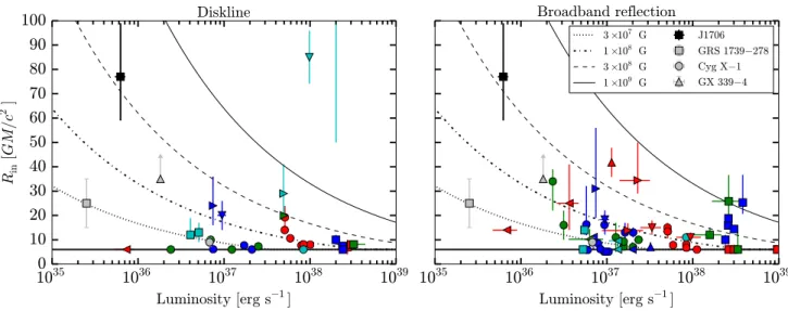
Figure 9. Overview of inner disc radius measurements as a function of bolometric X-ray luminosity (0.3–79 keV). The left-hand panel shows estimates with theDISKLINEmodel, while the right-hand panel contains broad-band reflection estimates (with e.g.RELXILLorREFLIONX). Each source has its own marker, listed in TableA1. The thick black line indicates the ISCO, assuming the Schwarzschild metric, while the other black lines show curves of constant magnetic field assuming a magnetically truncated disc. J1706 and the BHs are shown in both panels for easy comparison. In grey, we plot three examples of BH LMXBs. We stress that this plot only presents global trends, and cannot be used for detailed inferences due to differences in the individual analyses. For details on the sources, references, and caveats, see the Appendix.
lack of detected hydrogen is consistent with a WD donor. However,
we reiterate that a lack of Hαdoes not necessarily imply a compact
orbit – several LMXBs have been observed both with and without
Hαemission between different epochs [see Hern´andez Santisteban
et al. (2017) for a more detailed discussion] – and a VFXB with Hα
emission has been observed as well (Degenaar et al.2010). We also
note that several UCXB are not VFXBs (Heinke et al.2013). So
merely being an UCXB is not sufficient to be a VFXB, and VFXBs cannot form a single subset of a larger class of UCXBs.
6.1.2 Magnetic inhibition
An alternative proposed idea for the nature of persistently very faint accreting NSs is that of magnetic inhibition of the accretion flow
(Degenaar et al.2014,2017a; Heinke et al.2015). In this scenario,
the NS magnetic field is strong enough to truncate the accretion disc away from the ISCO and as such prevent efficient accretion. In such a geometry, the magnetic field might also launch a
propeller-driven outflow (e.g. Illarionov & Sunyaev1975). Through X-ray
reflection spectroscopy, the inner disc radius can be measured to search for such a disc truncation. However, disc truncation is not direct evidence for magnetic inhibition, especially at low accretion rates where the accretion flow changes structure: the inner accretion disc can transition into an RIAF, also effectively resulting in a
truncation of the thin disc (e.g. Narayan & Yi1994).
Distinguishing between the formation of such an RIAF and mag-netic truncation is problematic in a single source, but the comparison with the full sample of measured inner disc radii could help break
the degeneracy. Hence, we present such a comparison in Fig.9: both
panels show the measured inner disc radii versus X-ray luminosity of both a large sample of NSs and three BHs – the latter, contain-ing two BH LMXBs and the BH HMXB Cyg X-1, are selected for their coverage of the low X-ray luminosity regime (see the Ap-pendix). In the left-hand panel, we plot estimates of the inner disc
radius measured using theDISKLINEmodel, while in the right-hand
panel we plot those determined using broad-band reflection models
such asRELXILLorREFLIONX. We also include our inner disc radius
measurement for J1706 in both panels.
TheAppendix contains detailed information on source selection and the conversion to the used energy band (3–79 keV). In both pan-els, the black (dotted) lines indicate the predicted relation between inner radius and luminosity for a given magnetic field strength,
fol-lowing equation 1 in Cackett et al. (2009) and assuming magnetic
disc truncation.5We stress that, since the data points come from
a heterogenous set of analyses and publications with different un-derlying assumptions and caveats, these plots only present global trends and cannot be used for any detailed inferences. For important caveats and differences between the publications and assumptions, we refer the reader to the Appendix as well.
Due to observational challenges, the low X-ray luminosity re-gion of interest is highly undersampled, both in BHs and NSs: in addition to J1706, only a single inner radius measurement in an
NS LMXB has been made belowLX=1036erg s−1(Cackett et al.
2010). Prior analysis of high-qualityXMM–Newtonspectra in three
persistent VFXBs at even lower X-ray luminosities (Armas Padilla
et al.2013a) or two transient VFXBs (Armas Padilla et al.2011,
2013b) did not reveal any reflection features. Hence, the current data are not yet sufficient to distinguish between Advection-dominated accretion flow (ADAF) formation and disc truncation by the mag-netic field at low luminosities. In addition, other sources show a truncated disc at much higher luminosities, where ADAF formation is less likely (for instance the Rapid Burster and the Bursting Pul-sar), without being VFXBs; while a different type of disc-magnetic field interaction might be at play in those sources (such as a trapped
disc; D’Angelo & Spruit2010; Degenaar et al.2014; van den
Eijn-den et al.2017) and the Bursting Pulsar has a very wide (∼11.8 d)
orbit (Finger et al.1996), this shows that magnetic truncation is not
always sufficient to inhibit accretion and create a VFXB.
5We use standard geometrical and efficiency assumptions, and set
M=1.4 MandR=10 km.