William J. Porter1,∗ and Joaqu´ın E. Drut1,†
1
Department of Physics and Astronomy, University of North Carolina, Chapel Hill, North Carolina, 27599-3255, USA (Dated: September 10, 2018)
We characterize non-perturbatively the R´enyi entropies of degree n = 2,3,4, and 5 of three-dimensional, strongly coupled many-fermion systems in the scale-invariant regime of short interac-tion range and large scattering length, i.e. in the unitary limit. We carry out our calculainterac-tions using lattice methods devised recently by us. Our results show the effect of strong pairing correlations on the entanglement entropy, which modify the sub-leading behavior for large subsystem sizes (as characterized by the dimensionless parameter x=kFLA, where kF is the Fermi momentum and
LAthe linear subsystem size), but leave the leading order unchanged relative to the non-interacting
case. Moreover, we find that the onset of the sub-leading asymptotic regime is at surprisingly small x'2−4. We provide further insight into the entanglement properties of this system by analyzing the spectrum of the entanglement Hamiltonian of the two-body problem from weak to strong cou-pling. The low-lying entanglement spectrum displays clear features as the strength of the coupling is varied, such as eigenvalue crossing and merging, a sharp change in the Schmidt gap, and scale in-variance at unitarity. Beyond the low-lying component, the spectrum appears as a quasi-continuum distribution, for which we present a statistical characterization; we find, in particular, that the mean shifts to infinity as the coupling is turned off, which indicates that that part of the spectrum rep-resents non-perturbative contributions to the entanglement Hamiltonian. In contrast, the low-lying entanglement spectrum evolves to finite values in the noninteracting limit. The scale invariance of the unitary regime guarantees that our results are universal features intrinsic to three-dimensional quantum mechanics and represent a well-defined prediction for ultracold atom experiments, which were recently shown to have direct access to the entanglement entropy.
I. INTRODUCTION
This is an incredibly exciting time for research in ul-tracold atomic physics. The degree of control that ex-perimentalists have achieved continues to rise, year after year, along with their ability to measure collective prop-erties in progressively more ingenious ways (see e.g. [1– 4]). Indeed, after the realization of Bose-Einstein conden-sates over two decades ago [5–7] (see also [8]), followed by Fermi condensates in 2004 [9], the field entered an accelerated phase and rapidly developed control of mul-tiple parameters such as temperature, polarization, and interaction strength (in alkali gases via Feshbach reso-nances, see e.g. [10], and more recently in alkaline-earth gases via orbital resonances, see e.g. [11–13]), as well as exquisite tuning of external trapping potentials. Addi-tionally, multiple properties can be measured, ranging from the equation of state (see e.g. [14–16]) to hydrody-namic response (see e.g. [17, 18]) and, more recently, the entanglement entropy [19, 20].
This sustained progress has strengthened the intersec-tions with other areas of physics, in particular modern condensed matter physics and quantum information [21], as well as with nuclear [22] and particle physics [23– 25]. Quantum simulation by fine manipulation of nu-clear spins, electronic states, and optical lattices, now appears more realistic than ever [26–28]. At the
inter-∗Electronic address: [email protected] †Electronic address:[email protected]
face between many of those areas lies a deceptively sim-ple non-relativistic scale invariant system: the unitary Fermi gas, which corresponds to the limit of vanishing interaction ranger0and infinite s-wave scattering length a, i.e.
0←r0n−1a→ ∞ (1)
where n is the density; this regime corresponds to the threshold of two-body bound-state formation.
Both a model for dilute neutron matter and an ac-tually realized resonant atomic gas, this universal spin-1/2 system has brought together the nuclear [30–32], atomic [33], and condensed matter physics areas [34–36], as well as the AdS/CFT area [37–39], due to the under-lying non-relativistic conformal invariance [40]. While many properties of this quintessential many-body prob-lem are known (see e.g. [22] for an extensive review), other properties like entanglement and quantum infor-mation aspects have thus far remained unexplored, which brings us to our main point.
As this work is being written, quantum information concepts are increasingly becoming part of the mod-ern language of quantum many-body physics (see e.g. Refs. [21, 41–43]), in particular with regards to the char-acterization of topological phases of matter and quantum computation, but also in connection with black holes (see e.g. [44]) and string theory (see e.g. [45]). In the past decade or so, a large body of work has been produced characterizing the entanglement properties of low dimen-sional systems (especially those with spin degrees of free-dom [46–48]) at quantum phase transitions (in particular those with topological order parameters that defy a local
description) as well as systems of noninteracting fermions and bosons [49–53], which presented a challenge of their own.
With that new perspective in mind, in this work we set out to characterize the entanglement properties of the unitary Fermi gas using non-perturbative lattice meth-ods. We analyze the reduced density matrix, entangle-ment spectrum, and associated R´enyi entangleentangle-ment en-tropies of the two-body problem by implementing an ex-act projection technique on the lattice. For the many-body problem, we use a Monte Carlo method developed by us in Refs. [54, 55], based on the work of Ref. [56], to calculate the n-th R´enyi entanglement entropy. We showed in that work that our method overcomes the signal-to-noise problem of na¨ıve Monte Carlo approaches. We did that using the 1D Fermi-Hubbard model as a test case, but to our knowledge no previous calculations have been attempted for the challenging case of 3D Fermi gases.
The remainder of this paper is organized as follows: In Sec. II we present the main definitions and set the stage for Sec. III, where we explain how we carry out our calculations of the entanglement spectrum and en-tanglement entropies in two- and many-fermion systems. For completeness, we also include in that section a dis-cussion on how to avoid the signal-to-noise issue that plagues entanglement-entropy calculations in the many-body case. We extend that discussion to the case of bosons in the same section. In Sec. IV we show our re-sults for the entanglement spectrum and entropies of the two-body system along the BCS-BEC crossover, and in Sec. V we present the R´enyi entanglement entropies of many fermions at unitarity. We present a summary and our main conclusions in Sec. VI. The appendices contain more detailed explanations of our few- and many-body methods.
II. DEFINITIONS: HAMILTONIAN, DENSITY MATRICES, AND THE ENTANGLEMENT
ENTROPY
The Hamiltonian governing the dynamics of resonant fermions can be written as
ˆ
H = ˆT+ ˆV , (2)
where the non-relativistic kinetic energy operator is
ˆ
T = X
s=↑,↓
Z
d3rψˆ†
s(r)
−∇
2
2m
ˆ
ψs(r), (3)
where ˆψ†
s(r) and ˆψs(r) are the creation and annihilation
operators of particles of spins=↑,↓at locationr. The two-body, zero-range interaction operator is
ˆ V =−g
Z
d3rψˆ†
↑(r) ˆψ↑(r) ˆψ †
↓(r) ˆψ↓(r), (4)
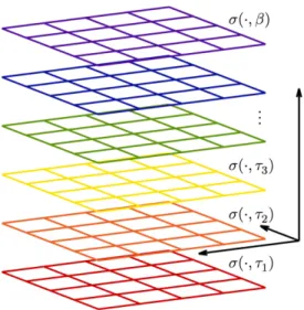
FIG. 1: The (bipartite) entanglement entropies computed in this work correspond to partitioning the system into a sub-systemA(in coordinate space, but it can also be defined in momentum space) and its complement ¯A. In practice, the calculations are carried out on systems that live in a cubic lattice of side L, and the subsystems are defined by cubic subregions of sideLA ≤L. The reduced density matrix ˆρA
of the open systemAcontains the information about entan-glement betweenAand ¯A, and is obtained by tracing the full density matrix over the states supported by ¯A, which form the Hilbert spaceHA¯.
where the bare couplinggis tuned to the desired physical situation. By definition, the limit of unitarity is achieved by requiring that the ground state of the two-body prob-lem lies at the threshold of bound-state formation (note that in 1D and 2D bound states form at arbitrarily small attractive coupling, but a finite value is required in 3D). Because our work was carried out in a finite volume with periodic boundary conditions, we used L¨uscher’s formal-ism [57, 58] to relate the bare coupling to the scattering length in the analysis of the BCS-BEC crossover. We describe that procedure below, when showing the results for the two-body problem.
The full, normalized density matrix of the system is
ˆ ρ= e
−βHˆ
Q , (5)
where
Q= TrH
h
e−βHˆi, (6)
is of course the canonical partition function, and H is the full Hilbert space. In this work we are concerned with systems in a pure state, namely the ground state
|Ξi, such that the full density matrix can be written as
ˆ
ρ=|ΞihΞ|. (7)
0 0.5 1 1.5 2 2.5 3 3.5 4 4.5
0.1 1 10 100 1000
d= 1
S2
(
x
)
x asymp.
N= 800 N= 400 N= 200 NN= 100= 50
0 0.5 1 1.5 2
0.1 1 10 100
d= 2
S2
(
x
)
/x
x asymp.
N = 5000 N = 2250 NN= 1000= 450 N= 200
0 0.1 0.2 0.3 0.4 0.5
0.1 1 10
d= 3
S2
(
x
)
/x
2
x asymp.
N= 3880 NN= 1150= 340 NN= 100= 30
FIG. 2: Second R´enyi entropy S2 of N non-interacting
fermions ind= 1,2,3 dimensions (top to bottom) as a func-tion of x=kFLA, whereA is a segment, square, and cubic
region, respectively, andLA is the corresponding linear size;
kF is the Fermi momentum. S2 is scaled by the surface area
dependence, namelyxandx2in 2D and 3D, respectively. The xaxis is plotted logarithmically to show that, up to finite-size effects, the results heal to the expected asymptotic regime of linear dependence with log10x(dashed line). This regime sets in at x '2−4 across all d. Finite-size effects appear as a sudden drop at largex.
A subsystemAand its complement ¯A(in coordinate or momentum space, see Fig. 1) support states that belong to Hilbert spacesHAandHA¯, respectively, such that the Hilbert space H of the full system can be written as a direct product space
H=HA⊗ HA¯. (8)
The density matrix ˆρAof subsystemA, usually referred
to as the reduced density matrix, is defined by tracing over the degrees of freedom supported by ¯A, i.e. tracing over the states inHA¯:
ˆ
ρA= TrH¯
Aρ.ˆ (9)
Based on this definition, the properties ofAas an open subsystem can be formulated and computed using oper-ators with support in A. In particular, a quantitative measure of entanglement between A and ¯A is given by the von Neumann entanglement entropy,
SvN,A=−TrHA[ˆρAln ˆρA], (10)
and by then-th order R´enyi entanglement entropy,
Sn,A=
1
1−nln TrHA[ˆρ n
A]. (11)
Naturally, these entropies vanish when A is the whole system, as then there is full knowledge of the state of the system. In any other case, the entanglement entropy will be non-zero, unless the ground state factorizes into a state living inAand a state living in ¯A. Because the en-tanglement betweenAand ¯Ahappens across the bound-ary that separates those regions, it is natural to expect Sn,A to be extensive with the size of that boundary, i.e.
proportional to the area delimiting A. This point was the topic of many papers in the last decade or so, espe-cially in connection with quantum phase transitions (see e.g. [59]).
It was rigorously shown in recent years, however, that the R´enyi entropy of non-interacting fermions with a well-defined Fermi surface presents a logarithmic viola-tion of the area law [49–53]. This abnormality was con-firmed numerically with the aid of overlap-matrix meth-ods [60], which we reproduce in Fig. 2, where we explic-itly show said logarithmic dependence (dashed line) as a function ofx=kFLA, wherekF is the Fermi momentum
andLAis the linear size of regionA, such that
x=kFLA =
πN 2
LA
L in 1D, (12)
= (2πN)1/2LA
L in 2D, (13)
= (3π2N)1/3LA
L in 3D, (14)
whereN is the total particle number. Note that, at large enoughx, finite size effects eventually take over and the entropy quickly tends to zero. The sub-leading oscilla-tions were studied in detail in Ref. [61].
Although resonant fermions are strongly coupled (the regime is non-perturbative and away from any regime with small dimensionless parameters), we can expect Sn,Ato follow a similar trend as the non-interacting gas,
the resonance), whose role in the entanglement entropy has been emphasized many times (see e.g. [62]). Sec-ond, our experience withSn,Afor the Hubbard model in
other cases [54] indicates that very strong couplingsU/t are needed even in 1D (where quantum fluctuations are qualitatively stronger than in 3D) in order for Sn,A to noticeably depart from the non-interacting result. Thus, we anticipate a similar behavior for resonant fermions as that of the bottom panel of Fig. 2; the latter provides some qualitative knowledge of where the leading loga-rithmic and sub-leading dependence sets in forSn,Aas a
function ofx=kFLA. In fact, as we will see below, the
onset of the asymptotic behavior (meaning dominated by leading and sub-leading dependence on x) at x'2−4 is the same for unitarity as for the non-interacting case. This is surprising, as there is no obvious reason for that to be the case: had this onset appeared atx' 10, the calculations in this work would not have been possible, as they would have required huge lattices. We return to this discussion below, when presenting our results for the many-body case.
III. METHOD
In this section we explain the two approaches used in this work. We address the two-body problem first, which we solved with a direct (i.e. non-stochastic) projection method on the lattice. This problem can be solved ex-actly by changing to center-of-mass and relative coordi-nates. However, doing so implies using a method that only works in that case, and we are interested in tech-niques that can be used in a variety of situations (e.g. in the presence of external fields, more than two parti-cles, time-dependent cases, and so forth). We then ad-dress the many-body problem using a method recently put forward by us, which we first presented and tested for one-dimensional systems in Ref. [55].
Although both approaches make use of an auxiliary field transformation, the ultimate utility of this technique is markedly different in each case. We detail below the portion of the formalism common to both approaches, treating in subsequent sections the details of their diver-gence from common assumptions and notation.
At chemical potentialµand inverse temperatureβ, the grand canonical partition functionZ is defined via
Z= Trhe−β( ˆH−µNˆ)i (15) for Hamiltonian ˆH and particle-number operator ˆN. Writing the inverse temperature as an integer number Nτ of steps, we implement a symmetric Suzuki-Trotter
decomposition with the goal of separating each operator into distinct one- and two-body factors. For the Boltz-mann factor, we obtain
e−β( ˆH−µNˆ) =
Nτ
Y
j=1
e−τK/ˆ 2e−τVˆe−τK/ˆ 2+
O(τ2) (16)
FIG. 3: Shown here is a representation of the lattice used in our calculations. Each horizontal lattice plane represents the 3D lattice where the system lives, and the vertical stacking of the planes represents the imaginary time direction. Although the original Hamiltonian is time-independent, the auxiliary fieldσthat represents the interaction is supported by a space-time lattice and induces a space-time dependence that disappears upon averaging.
were we define
ˆ
K= ˆT−µN .ˆ (17)
At each position r and for each of the Nτ factors,
we decompose the interaction via the introduction of a Hubbard-Stratonovich auxiliary fieldσ which we choose to be of a continuous and compact form [63, 64]. More specifically for each spacetime position (r, τj), where
r∈[0, L)3 andτ
j =jτ for some 1≤j≤Nτ, we write
eτ gnˆ↑nˆ↓=Z
π
−π
dσ
2π 11 +Bnˆ↑sinσ
11 +Bnˆ↓sinσ
(18)
having suppressed the spacetime dependence of the field σand the spatial dependence of the fermion density op-erators ˆns(r) = ˆψs†(r) ˆψs(r) wheres=↑,↓. Knowing that
ˆ
ns(r) is idempotent, it follows that
eτ gˆn↑nˆ↓= 1 + (eτ g−1)ˆn
↑nˆ↓, (19) which shows that the constantB satisfies
eτ g
−1 = B 2
2 . (20)
Collecting the integration measures, we obtain a path-integral form of the partition function accurate to quadratic order in the temporal lattice spacing, writing
Z=
Z
where
ˆ
U[σ] =
Nτ
Y
j=1 ˆ
Uj[σ], (22)
and the individual factors are ˆ
Uj[σ] =e−
τK/ˆ 2Y
r
11 +Bnˆ↑(r) sinσ(r, τj)
(23)
× 11 +Bnˆ↓(r) sinσ(r, τj)
e−τK/ˆ 2. (24) As the kinetic energy operator ˆTand the number oper-ator ˆN are already written as products of flavor-specific operators, we may partition the operator ˆU into individ-ual factors each of which assumes responsibility for the evolution of a particular fermion speciess=↑,↓. We do this by defining operators ˆTs, ˆNs, and ˆKsfors=↑,↓ by
ˆ Ts=
Z
d3rψˆ†
s(r)
−∇
2
2m
ˆ
ψs(r), (25)
ˆ Ns=
Z
d3rψˆ†
s(r) ˆψs(r), (26)
and ˆKs= ˆTs−µNˆs. We then write
ˆ
Uj,s[σ] =e
−τKˆs/2Y
r
11 +Bnˆs(r) sinσ(r, τj)
(27)
×e−τKˆs/2, such that
ˆ
U[σ] = ˆU↑[σ] ˆU↓[σ], (28) where
ˆ
Us[σ] = Nτ
Y
j=1 ˆ
Uj,s[σ]. (29)
Performing the required Fock-space trace, the expo-nential form of each factor in the above provides (see e.g. [65])
Z=
Z
Dσ det 11 +U↑[σ]
det 11 +U↓[σ]
, (30)
where we have suppressed higher-order contributions in τ (which are of orderτ2), and written a matrixU
s[σ] for
the restriction of each of the operators ˆUs[σ] to the
single-particle Hilbert space. Each of those matrices contains an overall factor of the fugacity
z≡eβµ. (31)
In what follows, we exhibit this factor explicitly and re-define the matricesUs[σ] to reflect this revision. In this
work, we exclusively treat unpolarized systems, and so we may treat the determinants as equivalent in derivations that follow by writing
Z=
Z
Dσdet2(11 +zU[σ]), (32)
and neglecting to denote the spin degree of freedom wher-ever context precludes confusion.
A. Direct lattice approach to the entanglement spectrum of the two-body problem
1. Identifying the transfer matrix
In order to illustrate the details as well as the generality of our technique, we show the main steps here in broad strokes and leave the details for Appendix A.
Using the above path-integral form of Z, we first iso-late the two-body sector. From the finite-temperature partition function Eq. (30), we may derive the conven-tional virial expansion in powers of the fugacity for each spin, which is given by
Z=
∞
X
N↑,N↓=0
zN↑
↑ z
N↓
↓ QN↑,N↓, (33)
where we have identified the coefficient of the Ns-th
power of the fugacity as the Ns-particle canonical
par-tition functionQN↑,N↓. Expanding the path-integral
ex-pression for the grand canonical partition function, we find that in terms of the matrixU[σ], the (1 + 1)-particle partition function is
Q1,1=
Z
Dσtr2U[σ]. (34)
The path integral inQ1,1above can be evaluated directly in a way that elucidates the form of the two-body trans-fer matrix. To that end, we define a four-index object from which the above squared trace may be obtained by suitable index contraction:
Rab,cd=
Z
DσU[σ]acU[σ]bd. (35)
The same four-index object, with indices properly con-tracted to account for antisymmetry, can be used to an-alyze the (2 + 0)-particle case.
We next write out each of the matrices U[σ] in its product form; that is, we reintroduce Eq. (22) in matrix form:
U[σ] =
Nτ
Y
j=1
Uj[σ]. (36)
For each contribution to theN-body transfer matrix, ex-actlyNfactors of the matrixU[σ] appear, and as a result each temporal lattice point appears in the integrand N times. Turning to the individual factors, we write each of the matrices Uj[σ] in such a way as to exhibit the
interaction. That is, we write
Uj[σ] =T Vj[σ]T, (37)
where
[T]kk0 =e−τ k 2/2
is the single-particle form of the kinetic energy operator defined above (in momentum space), and the (position-space representation of the) auxiliary external potential operator has matrix elements
Vj[σ]
rr0 = 1 +Bsinσ(r, τj)
δrr0. (39)
At this point, all matrix elements have been written out and can be shifted around as needed to carry out the path integral. The only non-zero results are obtained, of course, when an even number (in this N = 2 case no more than 2) of fieldsσ(r, τj) appear in the integrand for
the same values of (r, τj).
This undoing of the Hubbard-Stratonovich transfor-mation may seem a cumbersome or convoluted way to proceed, but it is useful in that it mechanically generates the correct expression for theN-body partition function for any particle content simply by differentiation of the fermion determinants. Moreover, this is accomplished without the need to deal with operator algebra and is easily generalized to bosons. In the 2-body case, in
par-ticular, the above procedure results in
Rac,bd=
h
MNτ
2
i
ac,bd, (40)
where we have naturally identified the transfer matrix in the two-particle subspace
[M2]ac,bd = KabKcd+ (eτ g−1)Iabcd, (41)
and where
Kij =
X
p
TipTpj, (42)
Iijkl =
X
p
TipTpjTkpTpl. (43)
The form of the transfer matrix lends itself to a use-ful diagrammatic representation, which we show for the two- and three-particle cases (the latter derived in Ap-pendix A) in Eqs. (44), (45) and (46).
[M2]ac,bd =
c a
d b
+ (eτ g −1)
c a
d b
(44)
[M3]abc,def =
c b a
f e d
+ (eτ g −1)
c b
a
f e d
(45)
c b
a
f e d
=
c b
a
f e d
+
c b
a
f e d
+
c b
a
f e d
(46)
2. Obtaining the ground state and the reduced density matrix
Having identified the transfer matrix allows us to de-sign a projection method to approach the ground state by repeated application ofM2. Proposing a guess state
|Ξ0i, we extract the true two-particle ground state |Ξi via
MNτ
2 |Ξ0i
Nτ→∞
−−−−−→ |Ξi. (47)
In practice, we compute the position-space wavefunction ξ(x↑, x↓) = hx↑, x↓|Ξi. Wavefunction in hand, we com-pute the matrix elements of the full density matrix ˆρ as
hx↑, x↓|ρˆ|x0↑, x0↓i = hx↑, x↓|ΞihΞ|x0↑, x0↓i (48) = ξ∗(x0↑, x0↓)ξ(x↑, x↓). (49) From these, the elements of the reduced density matrix ˆ
choosing for each particle either a position inAor in the complement ¯A, we compute
hs|ρˆA|s0i=
X
a∈Ass0
(|si ⊗ |ai)†ρˆ(
|s0
i ⊗ |ai), (50)
where, at each fixed pair of two-particle statess, s0, the sum is taken over all states|ai ∈ HA¯ such that the state
|si ⊗ |ai ∈ HA⊗ HA¯ (resp. |s0i ⊗ |ai ∈ HA⊗ HA¯) is consistent with the first (resp. second) index of the ma-trix element being evaluated. We have denoted this set asAss0. From this matrix, we compute the entanglement
spectrum σ( ˆHA), that is the spectrum of the
entangle-ment Hamiltonian defined
ˆ ρA=e
−Hˆ
A, (51)
as well as the von Neumann and R´enyi entanglement en-tropies.
B. Lattice Monte Carlo approach to the many-body problem
To address the many-body system, we implement the Monte Carlo version of the algorithm outlined above. The output of this algorithm, however, is not the ground-state wavefunction but rather the expectation value of the desired observable in a projected state. In our case, the observable is of course the entanglement entropy. To obtain it, crucial intermediate steps are required that go beyond conventional Monte Carlo approaches. We there-fore outline the basic formalism first, and then proceed to explain the additional steps required to calculateSn,A.
1. Basic formalism
Beginning with a largely arbitrary many-body state
|Ω0i, we evolve the state forward in imaginary time by an extentβ via
|Ω(β)i=e−βHˆ
|Ω0i, (52)
For large imaginary times, we have
|Ω(β)i−−−−→ |β→∞ Ωi, (53) where|Ωiis the true ground state provided thathΩ0|Ωi 6= 0.
For an operator ˆO, we may obtain the ground-state expectation value by studying the asymptotic behavior of the function
O(β) = 1
Z(β)hΩ(β/2)|Oˆ|Ω(β/2)i, (54)
with the zero-temperature normalization defined as
Z(β) =hΩ(β/2)|Ω(β/2)i=hΩ0|e −βHˆ
|Ω0i. (55)
As derived in detail earlier, we implement a symmetric factorization of the Boltzmann weight [c.f. Eq. (16)] in order to separate factors depending only on the one-body kinetic-energy operator from the significantly more com-plicated two-body potential-energy operator responsible for the effects of the interaction. Following this approx-imation, we again implement an auxiliary field transfor-mation [c.f. Eq. (18)] to represent the interaction factor. This allows us to write the ground- state estimator of Eq. (54) defined above in path integral form as
O(β) = 1 Z(β)
Z
Dσ Pβ[σ]Oβ[σ], (56)
while simultaneously demonstrating that
Z(β) =
Z
Dσ Pβ[σ]. (57)
We have identified a naturally emerging probability mea-surePβ[σ] computed as
Pβ[σ] =hΩ0|Uˆβ[σ]|Ω0i, (58)
with the operator ˆUβ[σ] defined as in Eq. (22) (setting
µ= 0 in the kinetic energy factor since particle number is fixed in this formalism). The integrand takes the form
Oβ[σ] =
hΩ0|Uˆβ/2[σ] ˆOUˆβ/2[σ]|Ω0i
hΩ0|Uˆβ[σ]|Ω0i
. (59)
Taking advantage of the arbitrariness of the initial state, we choose for|Ω0ia Slater determinant for each fermion species constructed from single-particle plane-wave states φj for 1 ≤j ≤ N/2 with N/2 = N↓ = N↑. With this assumption, we find that the probability takes the form
Pβ[σ] = det
2
Uβ[σ], (60)
with
[Uβ[σ]]kk0 =hφk|Uˆβ[σ]|φk0i, (61)
where the indicesk, k0 satisfy 1
≤k, k0
≤N/2.
2. Path integral form of the reduced density matrix, replica fields, and the R´enyi entropy
It was shown by Grover in Ref. [56] that the reduced density matrix can be written in terms of the fermionic creation and annihilation operators ˆc†,ˆc as a weighted average with respect to the probability measure Pβ[σ]
derived above. Specifically,
ˆ ρA,β =
Z
Dσ Pβ[σ] ˆρA,β[σ], (62)
where
ˆ
ρA,β[σ] = det 11−GA,β[σ]
×
exp
−
X
i,j∈A
ˆ c†i
h
logG−1
A,β[σ]−11
i
ijˆcj
It is important to note that ˆρA,β[σ] is the reduced
den-sity matrix of a system of non-interacting fermions in the external fieldσ. Expressions for non-interacting reduced density matrices were first derived in Refs. [66–68], but it was not until the much more recent work of Ref. [56] that those were combined into the non-perturbative form of Eq. (62) amenable to Monte Carlo calculations.
In the above, GA,β[σ] is the spatial restriction of the
(equal-time) one-body density matrix for either flavor to the regionAcomputed as
GA,β[σ]rr0 = N/2
X
a,b=1
[Uβ−1[σ]]abφ∗b(r, β/2)φa(r0, β/2),
(64) where
φa(r
0, β/2) =
hr0|Uˆβ[σ]|φai (65)
φb∗(r, β/2) = hφb|Uˆβ[σ]|ri. (66)
We suppress the imaginary-time β dependence in much of what follows with the understanding that calculations are to be performed in the limit ofβ→ ∞.
From this decomposed form of the reduced density matrix, an estimator for the n-th order R´enyi entropy can be derived. Becausen powers of ˆρA are needed, an
equal number of auxiliary fields will appear (the “replica” fields), which we will denote collectively asσ.
The final result (see Refs. [54–56, 69, 70]) takes the form
exp ((1−n)Sn,A) = TrHA[ρ n A] =
1 Zn
Z
DΣP[σ]Q[σ], (67) where (note the suppressedβ dependence)
P[σ] =P[σ1]P[σ2]. . . P[σn], (68)
with the observable being
Q[σ] = det2W[σ], (69)
with
W[σ] =
n
Y
j=1
(11−GA[σj])
"
11 +
n
Y
k=1
GA[σk]
11−GA[σk]
#
. (70)
We have adopted a notation such that, for functions or integrals of functions of multiple auxiliary fields, we write
F[σ] =F[σ1, σ2, . . . , σn], (71)
and
Z
DΣF[σ] =
Z
Dσ1Dσ2. . .Dσn F[σ], (72)
respectively.
Equation (70) poses the challenging task of inverting 11−GA, which can be very nearly singular, as pointed out
in Ref. [69]. Forn= 2, no inversion is required, because the equations simplify such that
Q[σ] = det2[(
11−GA[σ1])(11−GA[σ2]) +GA[σ1]GA[σ2]]. (73) However, for higher n there is no simplification of that kind and therefore it is less clear how one may avoid the problem. We solved this problem in Ref. [55] (see also [71–74]); the main point is realizing that
detW[σ] = detL[σ] detK[σ], (74)
where L[σ] is a block diagonal matrix (one block per replicak):
L[σ]≡diag [11−GA[σk]], (75)
and
K[σ]≡
11 0 0 . . . 0 −R[σn]
R[σ1] 11 0 . . . ... 0
0 R[σ2] 11 0 0 0
..
. . .. ... ... 11 ... 0 . . . 0 R[σn−1] 11
,
(76) where
R[σk] =
GA[σk]
GA[σk]−11
. (77)
Within the determinant of Eq. (74), we multiply K[σ] andL[σ] and define
T[σ]≡K[σ]L[σ] =11−DG[σ], (78)
whereG[σ] is a block diagonal matrix defined by
G[σ] = diag [GA[σk]], (79)
and
D≡
11 0 0 . . . −11 11 11 0 . . . 0 0 11 11 . . . 0
..
. . .. ... ... ... 0 . . . 0 11 11
. (80)
Equation (83) is the result that allows us to bypass the inversion of11−GA. Moreover, the form ofT[σ] is clearly
simpler than that ofW[σ]. For those reasons we useT[σ] in all of the many-body calculations presented here. This formulation allowed us to study R´enyi entropies as high asn= 5; higher are also possible.
For completeness, we present here the simplification for the bosonic case as well (and add a subindexB ac-cordingly), for which
and
WB[σ] = n
Y
j=1
(11 +GA[σj])
"
11−
n
Y
k=1
GA[σk]
11 +GA[σk]
#
.(82)
The analogous strategy to avoid inversion leads here to
TB[σ]≡11−DBG[σ], (83)
whereG[σ] is a block diagonal matrix defined by
G[σ] = diag [GA[σn]], (84)
and
DB ≡
−11 0 0 . . . 11 11 −11 0 . . . 0 0 11 −11 . . . 0 ..
. . .. ... ... ... 0 . . . 0 11 −11
. (85)
3. Signal-to-noise issues and how to overcome them
The path integral form of the R´enyi entropy Eq. (67) has a deceptively simple form: It seems obvious that one should interpretP[σ] as the probability density andQ[σ] as the observable being averaged. This, in some sense, is a trap: whileQ[σ] is crucially sensitive to correlations among the replica fields σk, P[σ] completely factorizes
across replicas (i.e. it is insensitive to said correlations). As a consequence, a Monte Carlo implementation sam-pling σ according to P[σ] will give outlandish values of Q[σ] that fluctuate wildly and may not converge to the expected value. This feature is what in the lattice QCD area is often called an overlap problem (see e.g. Refs [75, 76]). The present case is especially challenging in 2D and 3D, as the magnitude of Q[σ] is expected to grow exponentially with the size of the boundary of the subregionA (see e.g. [71, 72]).
Motivated by the similarity between the numerator of Eq. (67) and the conventional path-integral form of par-tition functions, we address the overlap problem by first differentiating with respect to a parameter, then using Monte Carlo methods to compute that derivative, and finally integrating at the end. We outline this procedure in detail in Ref. [55], and reproduce part of it here.
We introduce a parameter 0 ≤ λ ≤ 1 by defining a function Γ(λ;g) such that
Γ(λ;g)≡
Z
DΣP[σ]Qλ[σ]. (86)
Normalization ofP[σ] implies that
ln Γ(0;g) = 0, (87)
while Eq. (67) implies
ln Γ(1;g) = (1−n)Sn,A. (88)
−25
−20
−15
−10
−5 0
0 0.2 0.4 0.6 0.8 1
LA/L= 5/12,n= 2
h
ln
Q
[
σ
]
iλ
λ
N = 172 N = 136 NN= 104= 68 N = 34
FIG. 4: λ dependence of hlnQ[σ]iλ for a subsystem of size
LA = 5/12L, for N = 34,68,104,136,172 fermions at
uni-tarity in a box of sizeL=Nx`(whereNx = 12 points and
`= 1), and for R´enyi ordern= 2. Similar plots are obtained by varying, instead of the particle number, the region size and the R´enyi order. These are shown in Appendix B.
Using Eq. (86),
∂ln Γ
∂λ =
Z
DΣ ˜P[σ;λ] lnQ[σ], (89)
where
˜
P[σ;λ]≡ 1
Γ(λ;g)P[σ]Q
λ[σ] (90)
is a well-defined, normalized probability measure which features the usual weightP[σ] as well as an entanglement contribution Qλ[σ]. It is the latter factor that induces
entanglement-specific correlations in the sampling of σ when probability ˜P[σ;λ].
Thus, Sn,Ais calculated by usingλ= 0 as a reference
point and computingSn,Avia
Sn,A=
1 1−n
Z 1
0
dλhlnQ[σ]iλ, (91)
where
hXiλ=
Z
DΣ ˜P[σ;λ]X[σ]. (92)
We thus obtain an integral form of the interacting R´enyi entropy that can be computed using any MC method (see e.g. [63–65]), in particular hybrid Monte Carlo [77, 78] to tackle the evaluation ofhlnQ[σ]iλ as a function ofλ. In
practice, we find thathlnQ[σ]iλ is a smooth function of
λ, as exemplified in Fig. 4. It is therefore sufficient to perform the numerical integration using a uniform grid.
IV. RESULTS: TWO-BODY SYSTEM
0.1 1 10
−4 −3 −2 −1 0 1 2 3 4
a b c d e
0.1 1 10
a b c d e
λk
(kFa)−1 λ1 λ2 λ3 λ4 λ5
σ
(
ˆHA
)
FIG. 5: Bottom panel: Low-lying entanglement spectrum of the two-body problem as a function of the dimensionless coupling (kFa)−1in the BCS-BEC crossover, for a cubic
sub-regionAof linear sizeLA/L= 0.5. Top panels (a - e):
Low-lying (and part of the high) entanglement spectrum for se-lected couplings (a - e) at the top of the bottom panel.
continuum limit is approached by solving the problem for multiple lattice sizes, and by computing the renormal-ized coupling using the energy spectrum and L¨uscher’s formalism [57, 58]. The latter indicates that the relation-ship between the energy eigenvalues and the scattering phase shiftδ(p) is given by
pcotδ(p) = 1
πLS(η) (93)
whereη=pL2π andLis the box size, such that the energy of the two-body problem isE=p2/m; and
S(η)≡ lim Λ→∞
X
n Θ(Λ2
−n2) n2−η2 −4πΛ
!
, (94)
where the sum is over all 3D integer vectors, and Θ(x) is the Heaviside function. In turn, the scattering phase shift determines the scattering parameters via
pcotδ(p) =−1a+1 2reffp
2
+O(p4), (95)
where δis the scattering phase shift, a is the scattering length, andreff is the effective range.
A. Low-lying entanglement spectrum
Once the matrix elements of ˆρA are calculated from
the projected ground state, as shown above, we obtain the eigenvalues using standard diagonalization routines to obtain the entanglement spectrum σ( ˆHA), which is
defined as the spectrum of the entanglement Hamiltonian
0.6 0.7 0.8 0.9 1 1.1 1.2
−3 −2 −1 0 1 2
∆
(kFa)−1 LA/L= 1/10
2/10 3/104/10 5/10
FIG. 6: Schmidt gap ∆ between the two largest eigenvalues of the reduced density matrix, atLA/L= 0.1,0.2, ...,0.5 (top
to bottom), for the two-body system as a function of the coupling (kFa)−1
ˆ
HA, where
ˆ ρA=e−
ˆ
HA. (96)
In Fig. 5, we present our results forσ( ˆHA) for a cubic
subregionAof linear sizeLA/L= 0.5, for two particles in
the BCS-BEC crossover, parametrized by the dimension-less coupling (kFa)−1, wherekF is the Fermi momentum
(merely a measure of the particle density in the periodic box, as for two particles there is of course no Fermi sur-face) andais the s-wave scattering length. The latter was determined using the L¨uscher formalism outlined above. The main features of σ( ˆHA) can be described as
fol-lows. We note first that beyond the lowest 4 or 5 eigen-values, shown asλ1 toλ5 in the bottom panel of Fig. 5, the multiplicity of eigenvalues grows dramatically, form-ing a quasi-continuum. For this reason, we focus here on the lowest 5 eigenvalues and characterize the rest statis-tically in the next section. As is evident from the figure, the dependence of allλk on (kFa)−1 is rather mild and
smooth, although it has at a few crisp features: there is a rather large gap betweenλ1 and the next eigenvalue, which implies that the R´enyi entanglement entropies are dominated by that eigenvalue; there is a crossing ofλ2,λ3 andλ4on the BEC side of the resonance; after that cross-ingλ2 and λ3 heal to λ5 and effectively merge into the lower edge of the quasi-continuum part of the spectrum. The evolution of these properties along the crossover is shown in detail in panels a – e of Fig. 5.
In Fig. 6 we show the Schmidt gap ∆ (see Refs [79]), defined as the separation between the two largest eigen-values of the reduced density matrix ˆρA, for LA/L =
0.1,0.2, ...,0.5, as a function of (kFa)−1. Since we do
not expect a quantum phase transition as a function of (kFa)−1, we similarly do not expect the Schmidt gap
region 0<(kFa)−1<1. It is also evident that, because
λ1andλ4track each other at a very nearly constant sep-aration, the Schmidt gap becomes constant to the right of the sharp edge in Fig. 6. As with other features of this spectrum, it remains to be determined how ∆ evolves as a function of particle number, in particular as a Fermi surface forms and Cooper pairing correlations emerge.
As mentioned above, our calculations were carried out in a periodic box. We show the corresponding size ef-fects in Fig. 7, where we show the entanglement spec-trum of the two-body system as a function of the bare lattice coupling g. In that figure, it is clear that finite-size effects are smallest on the BCS side of the resonance, but become considerably more important on the BEC side. This is consistent with the expectation that, once a two-body bound state forms (as the coupling is increased away from the non-interacting point), the sensitivity to lattice-spacing effects is enhanced. It is noteworthy, in particular, that one may identify the unitary regime just by looking at this figure: for any given eigenvalue, the data for different lattice sizes crosses at about the same value ofg; this is reminiscent of the finite-size scaling be-havior of order parameters in critical phenomena, as it is the hallmark of scale invariance at phase transitions.
The process of reducing finite-size effects, at fixed par-ticle number, implies approaching the dilute limit, i.e. using larger lattices. When that limit is approached, the renormalization prescription that replacesgwith the physical coupling (kFa)−1(described above) should force
the finite-size calculations to collapse to a single, uni-versal (in the sense of size-independent) curve. This is indeed what we find and what yields the results of Fig. 5.
0.1 1 10
1 2 3 4 5 6 7 8 9 10
λ
g λ1
λ2, λ3 λ4 λ5
FIG. 7: Entanglement spectrum of the two-body problem in the BCS-BEC crossover as a function of the bare lattice coupling at different lattice sizes: solid, dashed, dotted, dash-dotted, forNx= 4,6,8,10, respectively. The subsystem size
was fixed toLA/L= 0.5. The coupling corresponding to the
unitary point is marked with a vertical dashed line. Note how different volumes cross precisely at unitarity, which reflects the property of scale invariance.
−5
−4
−3
−2
−1 0
1 2
3 5 10
15 20
25 0
50 100 cts.
(kFa)−1
λk cts.
10 12 14 16 18 20 22 24 26
−4 −3 −2 −1 0 1 2
8 12 16 20
−4−3−2−1 0 1 2
h
λk
i
(kFa)−1 LA/L= 5/10
LA/L= 4/10 LA/L= 3/10 LA/L= 2/10
h
λk
i
kFa
0 1 2 3 4 5 6 7 8
−4 −3 −2 −1 0 1 2
0 1 2 3 4 5
−4−3−2−1 0 1 2 σλ
k
(kFa)−1 σλ
k
kFa
FIG. 8: Top: Histogram of the high entanglement spectrum of the two-body problem showing number of counts (cts.) as a function of the coupling (kFa)−1and the entanglement
eigen-valueλk, for region sizeLA/L= 1/2. The dashed line shows
the dependence of the mean (see also middle plot). Middle and bottom: Mean and standard deviation, respectively, of the high entanglement spectrum distribution, as a functions of the interaction strength (kFa)−1(main) andkFa(inset). In
each plot the different curves show results for variousLA/L.
Note that the weak coupling limit corresponds tokFa→0−.
B. High entanglement spectrum
As mentioned in the previous section, the entangle-ment spectrum σ( ˆHA) above λ5, which we will refer
deem best to analyze using elementary statistical meth-ods. In Fig. 8, we show the eigenvalue distribution of the high entanglement spectrum for different system sizes, in histogram form. More importantly, we find that the mean and standard deviation of that distribution, shown here in Fig. 8 (middle and bottom), are smooth functions of (kFa)−1; the mean, in particular, diverges as the
cou-pling is turned off. We interpret this effect as strong evi-dence that the high sector ofσ( ˆHA) is a non-perturbative
component of ˆHAthat is entirely due to quantum
fluctua-tions induced by the interaction. Although the two-body system has no Fermi surface, it seems natural to con-jecture a link between Cooper pairing and the high en-tanglement spectrum. Determining whether this is true, however, is a challenging problem that requires studying the high entanglement spectrum in the progression from few to many particles.
Our numerical calculations show a large number of eigenvalues that lie far (at least 9 to 10 orders of magni-tude) above the high entanglement spectrum. While we cannot discard that those eigenvalues are consistent with numerical noise (they come from the lowest eigenvalues of the reduced density matrix), there are enough of them to warrant this brief comment. Although there is a large number of such eigenvalues, their contribution to the en-tanglement entropy is considerably suppressed by their small magnitude. We add to this discussion below.
C. Entanglement entropy
Using our knowledge of the eigenvalues λk ∈ σ( ˆHA),
the entanglement entropy of the two-body problem is eas-ily determined. Indeed, the von Neumann entropy is
SvN,A=−TrHA[ˆρAln ˆρA] =
X
k
λk e−λk, (97)
and then-th order R´enyi entanglement entropy is
Sn,A=
1
1−nln TrHA[ˆρ n A] =
1 1−nln
X
k
e−nλk. (98)
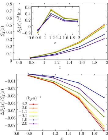
In Fig. 9 (top panel), we showS2 as a function ofx= kFLA and the coupling (kFa)−1. Remarkably, the trend
towards the leading asymptotic behavior proportional to x2lnxappears to set in atx
'2 for all couplings. This is surprising, as there is no obvious reason for this to be the case. As we will see below, we find the same kind of behavior for the many-body Fermi gas at resonance.
To show explicitly the effect of the high entanglement spectrum onS2, which we referred to in the previous sec-tion, we show in Fig. 9 (bottom panel) the contribution ∆S2 of the first entanglement eigenvalue to the full S2. It is clear in that plot that the contribution is at most on the order of 8% for the parameter ranges we studied.
0 0.1 0.2 0.3 0.4 0.5 0.6 0.7 0.8
0.6 0.8 1 1.2 1.4 1.6 1.8 2
−0.2 0 0.2 0.4 0.6
0.6 0.8 1 1.2 1.4 1.6 1.8 2 S2
(
x
)
x S2
(
x
)
/x
2ln
x
x
−0.07
−0.06
−0.05
−0.04
−0.03
−0.02
−0.01
0.6 0.8 1 1.2 1.4 1.6 1.8 2
(kFa)−1
∆
S2
(
x
)
/S
2
(
x
)
x 2.0
1.0
−0.1
−1.1
−2.0
−4.2
FIG. 9: Top: Second R´enyi entanglement entropy S2 of
the two-body problem as a function of x = kFLA and for
several values of the coupling (kFa)−1. Inset: S2 scaled by
x2lnx. Bottom: Relative contribution of the high entangle-ment spectrum to the second R´enyi entanglement entropyS2,
as a function ofx=kFLA.
V. RESULTS: MANY-BODY SYSTEM
Using the many-body lattice Monte Carlo techniques described above, along with the tuning procedure out-lined in the previous section, we computed several en-tanglement entropies of the unitary Fermi gas, aiming to characterize its leading and sub-leading asymptotic be-havior as a function of the subregion sizex=kFLA.
The results shown throughout this section were ob-tained by gathering 250 decorrelated auxiliary field con-figurations (where a single “auxiliary field” contains all the replicas required to determine the desired R´enyi en-tropy) for each value of the auxiliary parameterλ. We used particle numbers in the range N = 4−400 and cubic lattice sizes in the range Nx = 6−16 with
peri-odic boundary conditions. The projection to the ground state was carried out by extrapolation to the limit of large imaginary-time direction. The auxiliary parameter λwas discretized using Nλ= 10 points, which we found
to be enough to capture the very mild dependence on that parameter, as explained in a previous section (see also Appendix B for further details).
dis-cretization of spacetime, special attention was given to the ordering of the scales, to ensure that the thermo-dynamic and continuum limit were approached. Specifi-cally, we required the following ordering:
kF`1kFLAkFL, (99)
where ` = 1 is the lattice spacing, LA is the subsystem
size, andL=Nx`=Nxis the full system size. The first
condition on the left of Eq. (99) ensures that the con-tinuum limit is approached; the second condition implies that the region determined by LA must contain many
particles (since the density is the only scale in the sys-tem, this condition defines the large-LAregime); and the
last condition means that LA L, to ensure finite-size
effects are minimized. This ordering was accomplished by carefully choosing the restrictions onLAfor a given
par-ticle numberN, while aiming to maintain a largeN. The latter, however, requiresL to be large in order to avoid high densities where kF ' 1, which can be sensitive to
lattice-spacing effects. In addition, we setLA≤0.45Las
a compromise to satisfy the last inequality.
In Fig. 10 we show our results of the second R´enyi en-tropyS2of the unitary Fermi gas in volumes ofN3
xlattice
points, where Nx= 6−16, as a function ofx=kFLA,
for cubic subsystems of side LA. Within the statistical
uncertainty, shown in colored bands, the results for dif-ferent volumes coincide, which indicates that our results are in the continuum and thermodynamic regimes.
The inset of Fig. 10 showsS2scaled byx2in a semi-log plot. The fact that the trend is clearly linear supports the assertion thatxis large enough to discern the asymp-totic regime, where S2/x2
∝lnx. As in the case of the non-interacting Fermi gas, mentioned in the Introduc-tion, this onset of the asymptotic regime appears to be atx'2.
A. R´enyi entanglement entropies
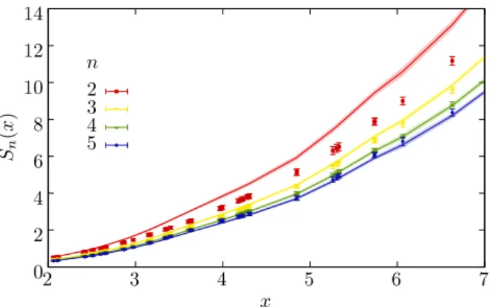
Using the formalism presented above for the deter-mination of R´enyi entanglement entropies for n ≥ 2, we computed Sn,A for the resonant Fermi gas for n =
2,3,4,5, as a function ofx=kFLA. In Fig. 11 we show
our main results. To interpret those results, we briefly discuss the noninteracting case. In Refs. [49–53] it was shown that the leading-order behavior or the entangle-ment entropy of non-interacting 3D fermions as a func-tion ofxis given by
Sn,A(x) =c(n)x2lnx+o(x2), (100)
where
c(n) = 1 +n −1 24(2π)d−1
Z
∂Ω
Z
∂Σ
dSxdSk|nˆx·nˆk| (101)
where Ω is the real-space regionAscaled to unit volume with normal ˆnx, Σ is the Fermi volume scaled by the
0.12 0.14 0.16 0.18 0.2 0.22
0 2 4 6 8 10
Nx
0.05 0.1 0.15 0.2 0.25 0.3 0.35
1 10
S2
(
x
)
/
(
x
2ln
x
)
x 16
14 12 108
6 S
2
(
x
)
/x
2
x
FIG. 10: Second R´enyi entropy of the unitary Fermi gas in units of x2lnx(main) and x2 (inset), wherex = kFLA.
Note the linear scale in the main plot and logarithmic scale in the inset. Although the range of values ofxis limited by our computational power (as set by method and hardware), the fact that the main plot is consistent with a straight line is a strong indication that the leading behavior of the entan-glement entropy as a function ofxis logarithmic. Moreover, we see that that behavior sets in as early asx ' 2, which is roughly consistent with the non-interacting case shown in Fig. 2.
Fermi momentum with unit normalnˆk. In our case, A is a cubic subsystem (as in Fig. 1) and a spherical Fermi volume.
The noninteracting case is shown in Fig. 11 in two ways. The asymptotic result at large x is shown with crosses on the right edge of the plot, extended into the plot (as a visual aid) with dashed black horizontal lines forn= 2,3,4,5 (top to bottom). With a thick red dashed line we show the casen= 2 at finitex, as obtained with the overlap-matrix method [60].
Our results for Sn,A for the unitary Fermi gas (data
points with error bands) appear to heal to the noninter-acting limit when the slow decay (see below) to a con-stant at large x is taken into account; this statement holds especially in then= 2 case where the sub-leading oscillations allow for a relatively clean fit. Indeed, our fits forn= 2 give
S2,A(x) =ax2lnx+bx2, (102)
witha= 0.114(2) andb= 0.04(1), while Eq. (101) yields c(2) = 3/(8π)'0.119366. . .. Whilec(2) are different to within our uncertainties, they are surprisingly close (be-tween 3 and 6%). The sub-leading behavior is consistent with an area law ∝ x2. As n is increased, sub-leading oscillations become increasingly apparent; however, they are mild enough that it is still possible to discern the asymptotic behavior at large x. For n = 3,4,5, oscil-lations notwithstanding, the results in the large-xlimit appear again to be close to the noninteracting case.
Using our results for the entanglement entropiesSn as
0.1 0.12 0.14 0.16 0.18 0.2 0.22 0.24
1 10 100
n 0.05
0.15 0.25 0.35
1 10
Sn
(
x
)
/
(
x
2 ln
x
)
x 2
3 4 5
Sn
(
x
)
/x
2
x
FIG. 11: R´enyi entropies of ordern= 2,3,4,5 (data points with error bands in red, yellow, green, and blue, respectively) of the unitary Fermi gas in units ofx2lnx(main plot) andx2 (inset), wherex=kFLA. Note the logarithmic scale in the
xaxis. The red dashed line shows the non-interacting result forn = 2, obtained using the overlap matrix method. The black dotted lines plotted over then= 2 data correspond to a fit the functional formf(x) =a+b/ln(x) (central line, with uncertainties marked by upper and lower dotted lines). The crosses on the right, and the corresponding horizontal dotted lines, indicate the expected asymptotic valuec(n) (from top to bottom, for n = 2,3,4,5) for a non-interacting gas (see Refs. [49–53]), which we reproduce in Eq. (101); numerically, they arec(2) = 0.11937...,c(3) = 0.10610...,c(4) = 0.09947..., andc(5) = 0.09549....
spectrum as a function of x. We studied the decay of (1−n)Sn/n to a constant value which, given Eq. (98),
we identified as −λ1. In Fig. 12 we show the result of using that sole eigenvalue to approximate Sn. As
ex-pected, higher ordersnemphasize the contribution from the lowest entanglement eigenvalue (highest eigenvalue of the reduced density matrix), which progressively domi-nates Sn as nincreases. From the n dependence ofSn,
it is also possible to study the degeneracy of the lowest entanglement eigenstate; at largen,
(1−n) n Sn'
lnd1
n −λ1+. . . , (103) where the ellipsis indicates exponentially suppressed terms, and d1 is the degeneracy associated with λ1. We find a vanishing first term, which indicates that d1 is consistent with unity.
VI. SUMMARY AND CONCLUSIONS
We implemented two different lattice methods to char-acterize non-perturbatively the entanglement properties of three-dimensional spin-1/2 fermions in the strongly interacting, resonant regime of short interaction range and large scattering length, i.e. the unitary limit. This regime is scale invariant (in fact, non-relativistic confor-mal invariant) in the sense that it presents as many scales
0 2 4 6 8 10 12 14
2 3 4 5 6 7
n
Sn
(
x
)
x 2
3 4 5
FIG. 12: R´enyi entanglement entropy Sn as a function of
x=kFLAforn= 2,3,4,5 (top to bottom). Monte Carlo
re-sults are shown as data points with error bars. The solid lines show the result of computingSnusing only the lowest
entan-glement eigenvalueλ1, i.e. the approximation Sn = nn−1λ1.
Uncertainties appear as shaded regions around the central value.
as non-interacting gases and therefore its properties are universal characteristics of three-dimensional quantum mechanics, i.e. in the same sense as critical exponents that characterize phase transitions.
We analyzed the two-body spectrum of the entangle-ment Hamiltonian along the BCS-BEC crossover and pre-sented results for the low-lying part, which displays clear features as the strength of the coupling is varied, such as eigenvalue crossing close to the resonance point and merging in the BEC limit. The lowest two eigenvalues in the spectrum correspond to the largest two eigenval-ues of the reduced density matrix, which are separated by the Schmidt gap. We found that the latter displays a sharp change at strong coupling, in the vicinity of the conformal point (kFa)−1= 0.
We also carried out a statistical characterization of the high entanglement spectrum, which appears as a quasi-continuum distribution with well defined mean and standard deviation, which we mapped out along the crossover. We found that the mean of the distribution tends to infinity in the noninteracting limit, which indi-cates that that sector is due to non-perturbative effects in the entanglement Hamiltonian. In contrast, the low-lying part of the spectrum has a finite noninteracting limit. All of the above two-body results were obtained with non-perturbative non-stochastic methods which are eas-ily generalizable to higher particle numbers (as we show analytically and diagramatically for 3 particles).
In addition, we studied the R´enyi entropies of degree n= 2,3,4, and 5 of many fermions in the unitary limit, which we calculated using a method recently developed by us (based on an enhanced version of the algorithm of Ref. [56]). We found that, remarkably, the largex= kFLA (i.e. subsystem size) limit for those entanglement
behavior using 2≤x≤10. For entropies of ordern >2, on the other hand, we found that sub-leading oscillations are enhanced, but not enough to spoil the visualization of the asymptotic behavior at largex.
Our experience with Monte Carlo calculations ofSn,A
in 1D gave us empirical indication that the entangle-ment properties of the unitary Fermi gas might not be too different from those of a non-interacting gas. How-ever, since unitarity corresponds to a strongly correlated, three-dimensional point, that intuition could very well have been wrong. Our calculations indicate that the leading-order asymptotic behavior is approximately con-sistent with that of a non-interacting system, while the sub-leading behavior is clearly different.
The recent measurement of the second R´enyi entropy of a bosonic gas in an optical lattice [19, 20] shows that it is possible to experimentally characterize the entan-glement properties of the kind of system analyzed here. Our calculations are therefore predictions for such ex-periments for the case of fermions tuned to the unitary limit.
Acknowledgments
This material is based upon work supported by the National Science Foundation under Grants No. PHY1306520 (Nuclear Theory Program) and PHY1452635 (Computational Physics Program). We
gratefully acknowledge discussions with L. Ram-melm¨uller.
Appendix A: Exact evaluation of the path integral for finite systems
In order to illustrate the details as well as the generality of this technique, we evaluate the path integral for a four-component tensor from which each of the above traces may be obtained by suitable index contraction.
To this end, we define
Rac,bd=
Z
DσU[σ]abU[σ]cd. (A1)
We first write out each of the matricesU[σ] in its product form. That is, we reintroduce the expression
U[σ] =
Nτ
Y
j=1
Uj[σ]. (A2)
For each contribution to theN-body transfer matrix, ex-actlyNfactors of the matrixU[σ] appear, and as a result each temporal lattice point appears in the integrand N times. Writing out the integrand and grouping by times-lice, we obtain
Rac,bd =
Z
DσU[σ]abU[σ]cd=
Z
Dσ U1[σ]U2[σ] . . . UNτ[σ]
ab
U1[σ]U2[σ] . . . UNτ[σ]
cd (A3)
= X
k1,k2,...,kNτ−1 l1,l2,...,lNτ−1
Z
DσU1[σ]ak1 U1[σ]cl1 U2[σ]k1k2 U2[σ]l1l2
. . . UNτ[σ]kNτ−1bUNτ[σ]lNτ−1d
(A4)
= X
k1,k2,...,kNτ−1 l1,l2,...,lNτ−1
Nτ
Y
j=1
Z
Dσ(τj)Uj[σ]kj−1kj Uj[σ]lj−1lj
, (A5)
where we set k0=a,l0=c, kNτ =b, andlNτ =d, and
used the notation
Dσ(τ)≡Y r
dσ(r, τ)
2π . (A6)
Using the specific form of the individualUfactors, we find
Z
Dσ(τj)Uj[σ]kj−1kjUj[σ]lj−1lj (A7)
=X
p,q p0,q0
Z
Dσ(τj)Tkj−1pVj[σ]pqTqkj
Tlj−1p0Vj[σ]p0q0Tq0l j
,
which using our chosen form ofVbecomes
=X
p,q p0,q0
Tkj−1pTqkjTlj−1p0Tq0ljδpqδp0q0 ×
Z
Dσ(τj) 1 +A sinσ(p, τj)
1 +A sinσ(p0, τj)
=X
p,q p0,q0
where we used
Z
Dσ(τj) 1 +A sinσ(p, τj)
1 +A sinσ(p0, τj)
= 1 + (eτ g
−1)δpp0. (A8)
Thus, we arrive naturally at the definition
[M2]ac,bd = KabKcd+ (eτ g−1)Iabcd, (A9)
as the transfer matrix in the two-particle subspace, where
Kij =
X
p
TipTpj, (A10)
Iijkl =
X
p
TipTpjTkpTpl. (A11)
Indeed, this definition ofM2as a transfer matrix makes sense, because
Rac,bd=
X
k1,k2,...,kNτ−1 l1,l2,...,lNτ−1
Nτ
Y
j=1
[M2]kj−1kj,lj−1lj, (A12)
or more succinctly,
Rac,bd=
h
MNτ
2
i
ac,bd. (A13)
In a similar fashion, one may show without much diffi-culty that the transfer matrix of the three-body problem
(for distinguishable particles, i.e. no symmetrization or antisymmetrization is enforced) is
[M3]abc,def =KadKbeKcf+ (eτ g−1)Jabc,def, (A14)
where
Jijk,lmn=KilIjkmn+KjmIikln+KknIijlm. (A15)
The pattern from this point on is clearly visible: there is one term for each ‘spectator’ particle that does not participate in the interaction, while the other two are accounted for by an interacting term governed by the
Iabcdobject. One may thus infer the form of the transfer
matrix for higher particle numbers.
Appendix B: Auxiliary parameter dependence
In this Appendix we show a few more examples on the mild dependence of the entanglement-entropy derivative
hlnQ[σ]iλ as other parameters are varied. In all cases, the data shown corresponds to full 3D calculations in the unitary regime.
In Fig. 13 (top) we show the variation of that derivative when the R´enyi order is changed from n= 2 to n= 5, at fixed particle number and region size. In Fig. 13 (bot-tom) we show howhlnQ[σ]iλ changes when the particle
number is varied, at fixed R´enyi ordern.
[1]Ultracold Fermi Gases, Proceedings of the Interna-tional School of Physics “Enrico Fermi”, Course CLXIV, Varenna, June 20 – 30, 2006, M. Inguscio, W. Ketterle, C. Salomon (Eds.) (IOS Press, Amsterdam, 2008). [2] I. Bloch, J. Dalibard, and W. Zwerger,Many-body physics
with ultracold gases, Rev. Mod. Phys.80, 885 (2008); [3] S. Giorgini, L. P. Pitaevskii, and S. Stringari,Theory of
ultracold atomic Fermi gases, Rev. Mod. Phys.80, 1215 (2008).
[4] M. Lewenstein, A. Sanpera, V. Ahufinger, Ultracold Atoms in Optical Lattices: Simulating Quantum Many-body Systems, (Oxford University Press, Oxford, 2012) [5] M. H. Anderson, J. R. Ensher , M. R. Matthews, C.
E. Wieman, E. A. Cornell,Observation of Bose-Einstein condensation in a dilute atomic vapor, Science269, 198 (1995).
[6] C. C. Bradley, C. A. Sackett, J. J. Tollett, R. G. Hulet, Evidence of Bose-Einstein Condensation in an Atomic Gas with Attractive Interactions, Phys. Rev. Lett. 75, 1687 (1995).
[7] K. N. Davies, M. O. Mewes, M. R. Andrews, N. J. van Druten, D. S. Durfee, D. M. Kurn, W. Ketterle, Bose-Einstein Condensation in a Gas of Sodium AtomsPhys. Rev. Lett. 75, 3969 (1995).
[8] G. Brumfiel, Focus: Nobel Prize – The Coolest Atoms, Phys. Rev. Focus8, 20 (2001).
[9] C. A. Regal, M. Greiner, and D. S. Jin, Observation of Resonance Condensation of Fermionic Atom Pairs, Phys. Rev. Lett.92, 040403 (2004).
[10] C. Chin, R. Grimm, P. Julienne, and E. Tiesinga Fesh-bach resonances in ultracold gases, Rev. Mod. Phys.82, 1225 (2010).
[11] G. Pagano, M. Mancini, G. Cappellini, L. Livi, C. Sias, J. Catani, M. Inguscio, and L. Fallani,Strongly Interacting Gas of Two-Electron Fermions at an Orbital Feshbach Resonance, Phys. Rev. Lett.115, 265301 (2015). [12] M. H¨ofer, L. Riegger, F. Scazza, C. Hofrichter, D. R.
Fernandes, M. M. Parish, J. Levinsen, I. Bloch, and S. F¨olling, Observation of an Orbital Interaction-Induced Feshbach Resonance in 173Yb, Phys. Rev. Lett. 115, 265302 (2015).
[13] S. Cornish,Viewpoint: Controlling Collisions in a Two-Electron Atomic Gas, Physics8, 125 (2016).
[14] M. J. H. Ku, A. T. Sommer, L. W. Cheuk, M. W. Zwier-lein, Revealing the Superfluid Lambda Transition in the Universal Thermodynamics of a Unitary Fermi Gas, Sci-ence335, 563 (2012).
[15] E. Cocchi, L. A. Miller, J. H. Drewes, M. Koschorreck, D. Pertot, F. Brennecke, and M. K¨ohlEquation of State of the Two-Dimensional Hubbard ModelPhys. Rev. Lett. 116, 175301 (2016).
Fermi-−70
−60
−50
−40
−30
−20
−10 0
0 0.2 0.4 0.6 0.8 1
LA/L= 5/12,N = 172
h
ln
Q
[
σ
]
iλ
λ
n= 5 n= 4 n= 3 n= 2
−20
−15
−10
−5 0
0 0.2 0.4 0.6 0.8 1
L= 12`,n= 2,N = 136
h
ln
Q
[
σ
]
iλ
λ
LA/L= 5/12 LA/L= 4/12 LA/L= 3/12 LA/L= 2/12
FIG. 13: Top: λdependence ofhlnQ[σ]iλfor several R´enyi
orders n = 2,3,4,5, for subsystem size LA = 5/12L, for
N = 172 fermions at unitarity in a box of size L = Nx`
(whereNx = 12 points and`= 1). Bottom: λdependence
of hlnQ[σ]iλ for several subsystem sizes LA, for N = 136
fermions at unitarity in a box of sizeL=Nx`(whereNx= 12
points and`= 1), and for R´enyi ordern= 2.
Hubbard ModelPhysics9, 44 (2016).
[17] C. Cao, E. Elliott, J. Joseph, H. Wu, J. Petricka, T. Sch¨afer, J. E. Thomas,Universal Quantum Viscosity in a Unitary Fermi Gas, Science331, 58 (2011).
[18] J. A. Joseph, E. Elliott, and J. E. Thomas, Shear Vis-cosity of a Unitary Fermi Gas Near the Superfluid Phase Transition, Phys. Rev. Lett.115, 020401 (2015). [19] R. Islam, R. Ma, P. M. Preiss, M. Eric Tai, A. Lukin,
M. Rispoli, and M. Greiner,Measuring entanglement en-tropy in a quantum many-body system, Nature528, 77 (2015).
[20] A. M. Kaufman, M. E. Tai, A. Lukin, M. Rispoli, R. Schittko, P. M. Preiss, M. Greiner, Quantum thermal-ization through entanglement in an isolated many-body system, arXiv:1603.04409.
[21] B. Zeng, X. Chen, D.-L. Zhou, X.-G. Wen,Quantum In-formation Meets Quantum Matter – From Quantum En-tanglement to Topological Phase in Many-Body Systems, arXiv:1508.02595.
[22]The BCS-BEC Crossover and the Unitary Fermi Gas, edited by W. Zwerger (Springer-Verlag, Berlin, 2012). [23] E. Zohar, J. I. Cirac, and B. Reznik, Quantum
simula-tions of gauge theories with ultracold atoms: Local gauge invariance from angular-momentum conservation, Phys.
Rev. A88, 023617 (2013).
[24] E. Zohar and M. Burrello Formulation of lattice gauge theories for quantum simulations, Phys. Rev. D 91, 054506 (2015).
[25] T. Pichler, M. Dalmonte, E. Rico, P. Zoller, and S. Mon-tangeroReal-Time Dynamics in U(1) Lattice Gauge The-ories with Tensor Networks, Phys. Rev. X 6, 011023 (2016).
[26] I. Bloch, J. Dalibard, S. Nascimb`ene,Quantum simula-tions with ultracold quantum gases, Nature Physics8, 267 (2012).
[27] I. M. Georgescu, S. Ashhab, and F. Nori,Quantum sim-ulation, Rev. Mod. Phys.86, 153 (2014).
[28] A. Reiserer and G. Rempe, Cavity-based quantum net-works with single atoms and optical photons, Rev. Mod. Phys.87, 1379 (2015).
[29] G. A. Baker, Jr.,Neutron matter model, Phys. Rev. C 60, 054311 (1999).
[30] Bertsch, G. F., 1999, in the announcement of the Tenth International Conference on Recent Progress in Many-Body Theories (unpublished).
[31] D. B. Kaplan, M. J. Savage, and M. B. Wise, A New Expansion for Nucleon-Nucleon Interactions, Phys. Lett. B424, 390 (1998).
[32] D. B. Kaplan, M. J. Savage, and M. B. Wise, Two-Nucleon Systems from Effective Field Theory, Nucl. Phys. B534, 329 (1998).
[33] K. M. OHara, S. L. Hemmer, M. E. Gehm, S. R. Granade, J. E. Thomas,Observation of a Strongly-Interacting De-generate Fermi Gas of Atoms, Science298, 2179 (2002). [34] D. Eagles, Possible Pairing without Superconductivity at Low Carrier Concentrations in Bulk and Thin-Film Superconducting Semiconductors, Phys. Rev. 186, 456 (1969).
[35] A. J. Leggett,Cooper pairing in spin-polarized Fermi sys-tems, J.Phys. (Paris) Colloq.41, C7 (1980).
[36] P. Nozieres and S. Schmitt-Rink, Bose condensation in an attractive fermion gas: From weak to strong coupling superconductivity, J. Low. Temp. Phys.59, 195 (1985). [37] K. Balasubramanian, J. McGreevy, Gravity duals for
non-relativistic CFTs, Phys. Rev. Lett. 101, 061601 (2008).
[38] D. T. Son,Toward an AdS/cold atoms correspondence: A geometric realization of the Schrdinger symmetry, Phys. Rev. D78, 046003 (2008).
[39] S. Kachru,Viewpoint: Glimmers of a connection between string theory and atomic physics, Physics1, 10 (2008). [40] Y. Nishida and D. T. Son,Nonrelativistic conformal field
theories. Phys. Rev. D76, 086004 (2007)
[41] L. Amico, R. Fazio, A. Osterloh, and V. Vedral, Entan-glement in many-body systems, Rev. Mod. Phys.80, 517 (2008).
[42] R. Horodecki, P. Horodecki, M. Horodecki, K. Horodecki, Quantum entanglement, Rev. Mod. Phys.81, 865 (2009). [43] J. Eisert, M. Cramer and M. B. Plenio,Colloquium: Area laws for the entanglement entropy, Rev. Mod. Phys.82, 277 (2010).
[44] M. Srednicki,Entropy and Area, Phys. Rev. Lett.71, 666 (1993).
[45] T. Nishioka, S. Ryu, T. Takayanagi,Holographic Entan-glement Entropy: An Overview, J. Phys. A 42, 504008 (2009).


![FIG. 4: λ dependence of hln Q[σ]i λ for a subsystem of size L A = 5/12L, for N = 34, 68, 104, 136, 172 fermions at uni-tarity in a box of size L = N x ` (where N x = 12 points and](https://thumb-us.123doks.com/thumbv2/123dok_us/8274763.2191461/9.918.474.831.82.304/fig-dependence-subsystem-size-fermions-tarity-size-points.webp)


![FIG. 13: Top: λ dependence of hln Q[σ]i λ for several R´ enyi orders n = 2, 3, 4, 5, for subsystem size L A = 5/12L, for N = 172 fermions at unitarity in a box of size L = N x ` (where N x = 12 points and ` = 1)](https://thumb-us.123doks.com/thumbv2/123dok_us/8274763.2191461/17.918.82.440.79.534/fig-dependence-orders-subsystem-fermions-unitarity-size-points.webp)
