conrad_yavuz_RoF_2016.pdf

(1)

Momentum and Reversal: Does What Goes

Up Always Come Down?*

Jennifer Conrad

1

and M. Deniz Yavuz

2

1

Kenan-Flagler Business School, University of North Carolina and2Krannert School of Management,

Purdue University

Abstract

The stocks in a momentum portfolio, which contribute to momentum profits, do not experience significant subsequent reversals. Conversely, stocks that do not contribute to momentum profits over the intermediate horizon exhibit subsequent reversals. Merging these separate securities into a single portfolio causes momentum and rever-sal patterns to appear linked. Stocks with momentum can be separated from those that exhibit reversal by sorting on size and book-to-market equity ratio. Controlling for proxies for behavioral biases, market illiquidity, and macroeconomic factors does not affect our results.

JEL classification: G10, G11, G12, G14, D03

1. Introduction

Momentum portfolio returns (Jegadeesh and Titman, 1993) are one of the most persistent,1

puzzling, and hence studied, patterns in finance. Many researchers have shown that a mo-mentum portfolio, which buys past winners and sells past losers, exhibits profits in the first 6–12 months. Other papers have shown that momentum profits are followed by reversals

or negative returns (Jegadeesh and Titman, 1993;Chan, Jegadeesh, and Lakonishok, 1996)

immediately after the first year, while longer-run reversals in 4–5 years are not significant

after controlling for Fama–French three factors (Fama and French, 1996).

* We are grateful for comments from Nicholas C. Barberis, Long Chen, Martijn Cremers, Zhi Da, Kent Daniel, Phil Dybvig, Huseyin Gulen, Byoung-Hyoun Hwang, Narasimhan Jegadeesh, Jonathan Lewellen, Ralitsa Petkova, Jacob Sagi, Charles Trzcinka, Sunil Wahal, and seminar participants at Purdue University, State of Indiana Conference, and Washington University in St Louis.

1 It is found in international markets (Rouwenhorst, 1998), in other asset classes (Asness, Moskowitz, and Pedersen, 2013), industries (Moskowitz and Grinblatt, 1999) and in out-of-sample periods (Carhart, 1997;Jegadeesh and Titman, 2001;Chabot, Ghysels, and Jagannathan, 2010). Persistence of these patters is especially puzzling given that momentum strategies are commonly associated with institutional investors (Grinblatt, Titman, and Wermers, 1995;Badrinath and Wahal, 2002).

VC_{The Authors 2016. Published by Oxford University Press on behalf of the European Finance Association. All rights} reserved. For Permissions, please email: [email protected]

Review of Finance, 2016, 1–27 doi: 10.1093/rof/rfw006

at Purdue University Libraries ADMN on August 5, 2016

http://rof.oxfordjournals.org/

(2)

Daniel, Hirshleifer, and Subrahmanyam (1998);Barberis, Shleifer, and Vishny (1998); andHong and Stein (1999)develop models that can explain both momentum and reversal patterns. These models’ ability to explain such time-series patterns is considered to be an

advantage over other theories,2_{which may explain intermediate-horizon momentum (see,}

e.g.,Berk, Green, and Naik, 1999), or long-horizon reversals (see, e.g.,Fama and French,

1996) but generally cannot explain both. However, evidence for a connection between

mo-mentum and reversals is not universal (see, e.g.,Rouwenhorst, 1998). It seems fair to say

that an explanation for momentum returns is still being debated. And, understanding the link between momentum and longer-horizon reversals is an important element of this debate.

Our main contribution is to show that there is no pervasive link between short-term mo-mentum and long-run reversals. Momo-mentum portfolio stocks that actually exhibit momen-tum in the short run do not exhibit reversal in the long run. In contrast, momenmomen-tum portfolio stocks that exhibit reversal in the short run continue to exhibit reversal in the long run. Merging these two sets of stocks into the momentum portfolio makes momentum and reversal patterns appear to be linked. In addition, we show that a momentum portfolio can be separated into subcomponent portfolios, which separately exhibit momentum and rever-sal, using stock characteristics at the time of portfolio formation. The component that ex-hibits momentum has returns that are large and persistent over time, do not show variation with proxies for behavioral biases, and are not explained by macroeconomic factors. In addition, this component is comprised of securities with relatively lower arbitrage costs.

We assume that, if momentum and reversal are linked, we should expect all “relative strength” portfolios to display both momentum and reversal patterns. Second, momentum and reversal patterns should happen consecutively. Third, stronger momentum should

pre-dict stronger reversals (Hirshleifer, 2001).

The standard momentum portfolio displays significant momentum in the 0–6 month interval and significant reversal in the 12–24 month interval. We begin by sorting momen-tum portfolio stocks into realized winners and losers based on the median of subsequent 6-month returns. The “realized momentum” portfolio includes original (past) winners that continue to be relative winners and original losers that continue to be relative losers in the first 6 months. The “contrarian” portfolio includes original winners (losers) that exhibit re-versal in the first 6 months. We find that conditional on being included in the realized mo-mentum portfolio, the probability of exhibiting reversal in the 12–24 month period is 46%, which is statistically significantly lower than 50%; securities that realize a momentum profit are less likely to exhibit reversal than we would expect by random chance.

Of course, reversal returns may be more attributable to those securities that experience momentum in the first 6 months. We find that the portfolio of stocks that exhibit momentum in the first 6 months does not exhibit statistically significant reversal in any horizon up to 5 years. In contrast, the contrarian portfolio displays significant reversal in risk-adjusted

re-turns in the 12–24 month period (–0.24% per month, t-statistic of 2.78). Therefore,

2 Differences in returns may be explained by cross-sectional variation in mean returns (Lo and MacKinlay, 1990;Conrad and Kaul, 1998), or by time-variation in expected returns (Berk, Green, and Naik, 1999;Chordia and Shivakumar, 2002;Johnson, 2002;Avramov and Chordia, 2006;Sagi and Seasholes, 2007;Liu and Zhang, 2008).

(3)

standard momentum portfolio reversals seem to be arising from persistence in the returns of

stocks that exhibit contrarian behavior in the first 6 months.3

The second part of the article examines whether we can identify stocksex antethat

ex-hibit persistent reversals, and those that experience momentum. The persistence in returns of realized momentum and contrarian portfolios suggests that characteristics, which have been shown to generate dispersion in returns, could be used to identify these stocks. We de-compose the standard momentum portfolio into separate portfolios based on independent sorts of past returns (winners and losers), and size and book-to-market equity ratio as char-acteristics (terciles), which proxy for expected returns. Specifically, we construct a portfolio (MAX), which shorts low expected returns losers that are relatively large or which have lower book-to-market equity ratios, while investing in high expected return winners that are relatively small or which have higher book-to-market equity ratios. In contrast, the min-imum portfolio (MIN) buys winner stocks with low expected returns and sells loser stocks with high expected returns. All other stocks are included in the NEUTRAL portfolio, which buys winners and sells losers with similar expected returns.

We find that MAX displays momentum but no reversal. Specifically, MAX’s average raw returns are 1.31% per month in the 0–6 month horizon (t-statistic of 6.43), and never exhibits significant reversals. In sharp contrast, MIN exhibits no evidence of momentum

and exhibits significant return reversals over the longer horizon: returns are 0.66%,

0.73%, and0.33% per month in the 6–12, 12–24, and 24–36 month horizons. The NEUTRAL portfolio displays both momentum and reversal patterns. However, the mo-mentum profits of the NEUTRAL portfolio occur only in the earlier half of our time period, while reversals occur only in the latter half of the sample. Therefore, even for the momen-tum portfolio formed from stocks with neutral characteristics, momenmomen-tum and reversal pat-terns do not appear to be linked, indicating that decoupling of the two patpat-terns is not driven solely by stock characteristics.

Mechanically, MAX and MIN load quite differently on size and book-to-market equity ratio. Therefore, we estimate the alphas of these portfolios after controlling for Fama– French three factors, estimating rolling regressions with these factors, conditioning factors on macroeconomic variables, and using characteristics-matched portfolio returns. The in-ferences remain the same.

We also examine the differences in MAX and MIN across other firm characteristics, including return on assets, the investment/sales ratio, leverage, R&D investment/sales, divi-dend growth, asset growth, accruals, and illiquidity. We find evidence of significant differ-ences between MAX and MIN in illiquidity, asset growth, investment/sales, and return on assets. As a consequence, we estimate alphas after controlling for investment, profitability,

and liquidity factors, using theFama and French (2015)five-factor model as well as the

Pastor–Stambaugh (2003)four-factor model. We obtain similar return patterns.

We test whether proxies shown to explain momentum such as lagged market returns (Cooper, Gutierrez, and Hameed, 2004), the investor sentiment index (Antoniou, Doukas, and Subrahmanyan, 2011), market illiquidity (Avramov, Cheng, and Hameed, 2014), or

3 Any explanation, such as a momentum life-cycle, that links momentum and reversal patterns implies that the realized momentum portfolio should exhibit reversal at some point in the future; we find no evidence of such a reversal in any subperiod out to 5 years. Unless such a life-cycle in mentum extends past 5 years, our evidence is more consistent with the simple explanation that mo-mentum and reversal patterns are not linked.

(4)

macroeconomic factors (Liu and Zhang, 2008) can explain the return patterns we docu-ment. We find that MIN returns load significantly on lagged market returns and an investor sentiment index, but MAX returns, which exhibit momentum, do not. This is consistent with other evidence that momentum profits are not explained by investment sentiment

measures (Moskowitz, Ooi, and Pedersen, 2012;Stambaugh, Yu, and Yuan, 2012). We

find that both MAX and MIN portfolio loser returns load positively and significantly on market illiquidity; this is not what one would expect if shorting constraints were driving

the results (although it is consistent with the results ofAvramov, Cheng, and Hameed,

2014). In fact, MAX losers are more liquid compared with MIN losers, implying that

MAX profits should be easier to arbitrage away. Macroeconomic factors explain a portion of the return continuation in the first 6 months for both portfolios and a portion of the re-versal in MIN returns between 12 and 24 months. Regardless, the time-series patterns and the decoupling of momentum and reversal patterns always remain in our results.

Our results indicate that momentum and reversals are separate phenomena. We find that the differences in characteristic-adjusted MAX and MIN returns are positive, and rela-tively stable, declining monotonically over the 3-year horizon. Our results point to an inter-action between characteristics and past returns, which may proxy for an omitted risk factor, or a behavioral bias that does not generate mispricing and correction, as a potential

explanation for momentum profits.4

2. Are Momentum and Reversal Patterns Linked?

If momentum and reversal patterns are linked, the primary predictions are that, on average, a winner (loser) from the formation period will over- (under-)perform in the intermediate term, and then go on to under- (over-)perform; reversals should follow momentum. In add-ition, under the assumption of segmented markets, the stronger the continuation in the

intermediate horizon, the stronger the reversal should be (Hirshleifer, 2001).

2.1 Standard Momentum Portfolio Time-Series Return Patterns

We consider all stocks (share codes 10 and 11) trading on the NYSE, Amex, and Nasdaq between January 1965 and December 2010 in the CRSP database. We employ the method ofLo and MacKinlay (1990)such that the weight of each stock within the loser and winner portfolios is determined by the absolute difference of its prior 6-month return from the average prior 6-month return of all stocks. This method ensures that we have a large num-ber of stocks in each portfolio when we use portfolios formed by the intersection of past re-turns and characteristics sorts in subsequent analysis. We categorize a stock as a winner (loser) if its prior 6-month return is higher (lower) than the average prior 6-month return of all stocks. We skip a month after portfolio formation in order to avoid market microstruc-ture issues.

InTable I, we present the returns to winner, loser, and winner–loser portfolios using all

stocks. We find that the winner minus loser (WL) portfolio earns 0.50% per month.

Controlling for Fama–French factors does not explain these returns; in fact, the alpha for the momentum strategy increases, to 0.65% per month. Following the initial 6-month

hold-ing period,WLreturns are flat in the following 6 months (months 6–12), and then

re-verse: average monthly returns in months 12–24 are0.36% per month (with at-statistic

4 Asness (1997)argued that such an interaction may exist between momentum and value.

(5)

of3.63) and continue to experience weak reversals in months 24–36 (0.16% per month,

with at-statistic of1.73). Returns over a longer horizon of 36–48 months are not

signifi-cant although there is some weak reversal in year 5 with a monthly return of0.15% per

month (the t-statistic is1.73). Once we control for Fama–French three factors, longer

horizon reversals in years 4–5 are insignificant (consistent withFama and French, 1996),

but the reversal returns immediately after the first year are0.22% per month and

signifi-cant (with at-statistic of1.99).

Overall, the momentum and reversal patterns observed inTable Iare consistent with

the results presented in previous papers (e.g.,Jegadeesh and Titman, 1993,2001;Chan,

Jegadeesh, and Lakonishok, 1996): portfolios formed using prior intermediate-horizon re-turns exhibit continuation in the following 6 months, followed by reversal over the next 2– 3 years.

2.2 Do Stocks Exhibit Reversal After Exhibiting Momentum?

If momentum and reversals patterns are linked, we expect stocks that exhibit momentum in the 0–6 month period to be more likely to exhibit reversal in the 12–24 month period. To examine whether momentum and reversal returns are generated by the same securities, we separate the momentum portfolio into two subcomponents. The “realized momentum” Table I.Standard momentum portfolio returns

The table shows monthly returns for the winner, loser, and winner minus loser portfolios for

the 0–6, 6–12, 12–24 and 24–36 month holding periods. Panel A shows monthly alphas with re-spect to Fama–French three factors and Panel B shows raw returns. The sample consists of all

NYSE, Amex, and Nasdaq stocks between January 1965 and December 2010. A stock is catego-rized as winner(loser) if its past 6 month return is higher(lower) than average past 6 month

re-turn of all stocks. A stock’s weight in a portfolio is determined by the absolute difference between stocks’ past 6 month return and the average past 6 month return of all stocks. Weights

are normalized to sum up to 1 within loser and winner portfolios. We skip 1 month between the portfolio formation period and the subsequent holding period. Thet-statistics are calculated using Newey–West standard errors with 12 months lag and reported in the second row.

0–6 6–12 12–24 24–36 36–48 48–60 months months months months months months

Panel A: All stocks monthly Fama–French three factor alphas

Winner 0.36 0.04 0.20 0.18 0.10 0.19 3.64 0.51 2.55 2.43 1.20 2.44 Loser 0.30 0.12 0.01 0.06 0.09 0.05

2.16 0.99 0.14 0.68 1.08 0.64

Winnerloser 0.65 0.08 0.22 0.12 0.01 0.14 3.96 0.55 1.99 1.32 0.17 1.68 Panel B: All stocks monthly raw returns

Winner 1.07 0.57 0.42 0.41 0.45 0.39

3.43 1.97 1.49 1.60 1.75 1.59

Loser 0.57 0.68 0.78 0.57 0.46 0.53

1.67 2.10 2.71 2.18 1.91 2.59 Winnerloser 0.50 0.11 0.36 0.16 0.00 0.15 2.76 0.75 3.63 1.73 0.06 1.73

(6)

portfolio includes past winners and losers that exhibit momentum in the first 6 months, that is, past winners that are winners and past losers that are losers. The “contrarian” port-folio includes stocks that exhibit reversal in the first 6 months, that is, past winners that are losers and past losers that are winners.

If reversal follows momentum, we expect stocks in the “realized momentum” portfolio

to be more likely to exhibit reversals in the 12–24 month period.Table IIshows that 46%

of original (past 6 month) winners, and 58% of original losers, continue as winners and los-ers, respectively, in the subsequent 6-month period. Of realized momentum winnlos-ers, 59.6% go on to experience some reversal; of the realized momentum losers, 38.9% reverse. On average, 46% of realized momentum stocks exhibit some reversal, which is statistically significantly less than the 50% we would expect if there were no relation between the

likeli-hood of momentum and subsequent reversals (p-value¼0.00 using the binomial

distribu-tion). By comparison, 50% of the securities in the contrarian portfolio experience reversals in the 12–24 month period. That is, instead of securities that experience momentum being more likely to reverse, the stocks that do not contribute to momentum are more likely to experience reversals.

Of course, it may be that the reversal returns generated by “realized momentum” securities are larger in magnitude. We examine the returns of “realized momentum” and “contrarian” portfolios over the subsequent 12–24 month period. Return continuation and reversals are considered anomalous to the extent that they are not explained by known risk factors.

Therefore, we consider Fama–French three factor-adjusted returns.Table IIIreports

risk-ad-justed returns of the portfolios in the 12–24 month period after portfolio formation—the period in which the standard momentum portfolio exhibits significant reversal. We find that the realized momentum portfolio does not exhibit statistically significant reversal in the 12–24 month period. In contrast, the contrarian portfolio displays significant reversal in the 12–24

Table II.Fraction of stocks that follow momentum and reversal patterns

The table reports probability of being categorized as high or low return stocks in the portfolio holding periods of 0–6 months and 12–24 months conditional on being high or low return stock

in the previous period. We useLo–MacKinlay (1990)methodology where a stock is categorized as winner(loser) if its past 6 month return is higher(lower) than average past 6 month return of

all stocks. The sample consists of NYSE, Amex, and Nasdaq stocks between 1965 and 2010. We skip 1 month between the portfolio formation period and the subsequent holding period.

6 to 0 0 to 6 12 to 24 6 to 0 0 to 6 12 to 24 months months months months months months

High 43.7%

High 46.4%

High 41.4%

Low 56.3%

High 41.6%

High 41% Low

59.6%

Low 59%

Low 53.6%

High 40.2%

Low 58.4%

High 38.9% Low

59.8%

Low 61.1%

(7)

month period, with an alpha of0.28% per month and at-statistic of2.69. The evidence in Table III, Panel B shows that similar results are obtained using theJegadeesh and Titman (1993)methodology.

To further explore return persistence, we rank these stocks into deciles based on their first 6-month holding period return, subsequent 12–24 month and 24–36 month returns and examine the correlations among relative return rankings. The correlations are always positive and significant across all horizons (results available upon request).

In summary, the evidence indicates that stocks in the component portfolios, on average, display persistence in relative returns in the portfolio evaluation period rather than momen-tum followed by reversal. More importantly, stocks that contribute to momenmomen-tum and re-versal returns are distinct—that is, we find relatively little evidence, in either the fraction of securities or in their returns, that securities which experience momentum in the first 6 months are more likely to experience subsequent reversals.

Table III.Do stocks that exhibit momentum reverse?

The table reports monthly alpha with respect to Fama–French three factors of momentum

folios formed from winner and loser stocks that exhibit momentum (realized momentum port-folio) versus stocks that exhibit reversal (contrarian portport-folio) in the first 6 months after

portfolio formation. Panel A usesLo–MacKinlay (1990)methodology where A stock is catego-rized as winner(loser) if its past 6 month return is higher(lower) than average past 6 month

re-turn of all stocks. A stock’s weight in a portfolio is determined by the absolute difference between stocks’ past 6 month return and the average past 6 month return of all stocks. Panel B

usesJegadeesh and Titman (1993)methodology of categorizing stocks into extreme winner and loser deciles according to their past 6 month returns. We also drop stocks under price of

five dollars at the time of portfolio formation. To be included stocks need to have prior 6 month returns and 0–6 month returns. The sample consists of NYSE, Amex, and Nasdaq stocks

be-tween 1965 and 2010. We skip 1 month bebe-tween the portfolio formation period and the subse-quent holding period. The t-statistics are reported in the second row and calculated using Newey–West standard errors with 12 months lag.

Realized momentum portfolio Contrarian portfolio Realized minus contrarian

Time Winnerloser t-stats Winnerloser t-stats Returns t-stats

Panel A:Lo and MacKinlay (1990)methodology

0–6 months 8.14 24.21 7.07 29.01 15.21 27.94 6–12 months 0.79 4.31 0.32 2.47 1.10 5.11 12–24 months 0.18 0.89 0.24 2.78 0.26 1.99 24–36 months 0.19 1.36 0.12 1.62 0.07 0.51 36–48 months 0.04 0.42 0.02 0.27 0.07 0.57 48–60 months 0.15 1.15 0.10 1.40 0.05 0.45 Panel B:Jegadeesh and Titman (1993)methodology

0–6 months 8.78 24.7 7.53 25.91 16.32 27.3 6–12 months 1.07 4.68 0.13 0.82 1.20 4.81 12–24 months 0.11 0.61 0.23 1.99 0.34 2.27 24–36 months 0.18 0.89 0.11 1.17 0.07 0.40 36–48 months 0.03 0.23 0.07 0.63 0.10 0.63 48–60 months 0.18 0.98 0.13 1.01 0.06 0.44

(8)

2.3 Alternative Explanations

This evidence could be consistent with more complex theories of momentum, which still in-dicate a link between momentum and reversals. As one example, it may be that the port-folios we construct are capturing securities that are in different phases of a “momentum

life-cycle”, as inLee and Swaminathan (2000). Specifically, our realized momentum

port-folio may include securities that are relatively early in their momentum life-cycle, while the contrarian portfolio includes securities that have already begun to reverse. Another alterna-tive explanation is that the stocks that are included in the realized momentum portfolio are selected by double sorting on momentum and hence may be more likely to exhibit persist-ence or continuation.

Regardless, any explanation that argues a link between momentum and reversal implies that the realized momentum portfolio should go on to exhibit reversal in the long(er) run.

We examine this possibility.Table IIIshows that the realized momentum portfolio does not

exhibit any significant reversal up to 5 years after portfolio formation. In fact, there is no statistical difference between the realized momentum and contrarian portfolio returns after the first 2 years. Assuming that the momentum life-cycle (for any security exhibiting mo-mentum) is no longer than 5 years, the evidence continues to suggest that momentum and reversal patterns are not linked.

3. Identifying Stocks with Momentum versus Reversals

The results inTable IIIindicate that momentum and reversal returns arise from different

stocks. If we can identify, at the time of portfolio formation, those securities that are likely to experience momentum or reversal, we may be able to better understand the sources of these return patterns.

The persistence in return rankings that we observe in the previous section could be a re-sult of differences in the expected returns of these stocks. To explore this issue, we form

size and book-to-market ratio-based portfolios that differ in expected returns (seeBanz,

1981;Fama and French, 1992). We use size at the time of portfolio formation and the

book-to-market equity ratio calculated as inFama and French (1992). We drop stocks that

have negative book-to-market equity ratio at the time of portfolio formation. We sort stocks into terciles based on these characteristics. We classify stocks into the high risk group if the stock is included in the high risk group (small market capitalization or high book-to-market equity) according to at least one characteristic and included in at least the medium risk category using the other characteristic. We classify stocks into the low risk group if the stock is included in the lowest risk group according to at least one characteristic and included at most in the medium risk category using the other characteristic. All other stocks are categorized in the medium risk group.

We create portfolios at the intersection of characteristic or risk terciles and momentum winners and losers. MAX invests in the highest risk tercile winners and lowest risk tercile losers, that is, MAX buys high market and small winners and sells low book-to-market and large losers. In contrast, the MIN portfolio invests in lowest risk tercile winners and highest risk tercile losers. Finally, the NEUTRAL portfolio includes stocks that are not categorized into either MAX or MIN. As a consequence, the winner and loser sides of the NEUTRAL portfolio should have relatively similar stock characteristics.

We may inadvertently sort stocks based on other characteristics that are correlated with

size or book-to-market equity ratio.Table IVprovides summary statistics of our MAX,

(9)

T able IV . Summary statistics of portfolios formed by characteristics and momentum The table provides summary statistics of stocks in MAX, MIN, and NEUTRAL portfolios winner and loser sides. Panel A provides median values, while Pane lB provides weighted quintiles of characteristics, where weights are based on past 6 months returns of stocks, across the entire sample period. MAX is a zero in-vestment portfolio, which buys the past winners in the highest expected return tercile and sells the past losers in the lowest expected return tercile . MIN is a zero investment portfolio, which buys the past winners in the lowest expected return tercile and sells the past losers in the highest expected return tercile. NEUTRAL include the middle risk winners minus middle risk losers. Stocks are sorted into expected return terciles using stock characteristics book-to-market and size. We first sort stocks into terciles using size and book-to-market independently. We classify stocks into the high risk group if the stock is inc luded in the high risk group according to at least one characteristic and included in at least medium risk by the other characteristic. We classify stocks into the low risk group if the stock is included in the lowest risk group according to at least one characteristic and included at most in the medium risk by the other characteri stic. All other stocks are categorized in the medium risk group. A stock is categorized as winner(loser) if its past 6 month return is higher(lower) than average past 6 month return of all stocks. Characteristics that use accounting values are calculated as in Fama and French (1992) . Size is the stock market capitalization at the time of portfolio formation. Book-to-market is calculated as in Fama and French (1992) . Investment/sales is capital expenditures divided by sales. Returns on assets is equal to net income divided by total assets. Leverage is debt in current liabilities plus long-term debt divided by total assets. R&D expense s/Sales is equal to R&D expenses divided by sales. Dividend growth is total dividend growth over the prior year. Asset growth is total asset growth over the prior y ear. Accruals is change in non-cash current assets minus change in current liabilities minus depreciation and amortizations as in Hirshleifer, Hou, and Teoh (2009) . Illiquidity ( Amihud, 2002 ) is measured over a month at the time of portfolio formation. The sample consists of NYSE, Amex, and Nasdaq stocks between 1965 and 2010. Portfolio Size Book-to-market Investment/ Sales Return on assets Leverage R&D expenses/sales Dividend growth Asset growth Accruals Illiquidity Average number of stocks Panel A: Medians (unless otherwise stated) MAX 25 1.30 0.03 0.02 0.21 0.01 0.00 0.03 1.07 1.02 555 winners MAX 383 0.38 0.05 0.06 0.17 0.04 0.09 0.13 2.6 0.02 753 losers MIN 512 0.41 0.05 0.06 0.17 0.04 0.09 0.12 3.0 0.01 670 winners MIN 16 1.20 0.03 0.02 0.22 0.01 0.00 0.04 0.9 2.14 790 losers (continued)

(10)

T able IV . Continued Portfolio Size Book-to-market Investment/ Sales Return on assets Leverage R&D expenses/sales Dividend growth Asset growth Accruals Illiquidity Average number of stocks NEUTRAL 122 0.77 0.04 0.04 0.21 0.02 0.05 0.07 1.8 0.09 439 winners NEUTRAL 57 0.58 0.04 0.03 0.21 0.03 0.04 0.07 0.96 0.30 596 losers Panel B: Characteristics quintiles weighted by relative past 6 months returns MAX 1.94 4.33 2.53 2.24 3.09 2.76 1.79 2.42 3.00 3.64 555 winners MAX 3.85 1.74 3.22 3.33 2.81 3.12 2.26 3.45 3.00 2.11 753 losers MIN 4.01 1.84 3.14 3.29 2.80 3.12 2.24 3.26 2.92 1.85 670 winners MIN 1.61 4.10 2.67 2.27 3.17 2.74 1.81 2.62 3.04 4.09 790 losers NEUTRAL 3.02 2.98 2.87 2.65 3.08 2.95 1.97 2.78 2.94 2.68 439 winners NEUTRAL 2.31 2.28 3.02 2.58 3.00 3.03 1.98 2.90 3.00 3.44 596 losers

(11)

MIN, and NEUTRAL portfolios across various characteristics including size, book-to-mar-ket ratio, return on assets, investment/sales, leverage, R&D investments/sales, dividend

growth, asset growth, accruals (as inHirshleifer, Hou, and Teoh, 2009), and illiquidity

(Amihud, 2002) (variable definitions are inTable IV). Panel A reports medians of charac-teristics, whereas Panel B first sorts stocks into quintiles based on characteristics and then calculates weighted averages of quintile categories, where weights are based on the past

6-month returns as in our portfolio return calculations.5

By construction, MAX winners have a smaller size and a higher book-to-market ratio than MIN winners, and MAX losers have higher market capitalization and smaller book-to-market ratios than MIN losers. There are also some differences across portfolios based on return on assets, investment/sales, asset growth, and illiquidity. We control for these dif-ferences in subsequent analyses.

As an advantage of using theLo and MacKinlay (1990)methodology, which includes

all stocks in the analysis, our portfolios continue to be well diversified. The average number of securities in these portfolios changes between 439 (NEUTRAL winners) and 790 (MIN losers); the minimum number of securities in any portfolio in any interval is 72.

We use independent sorts of characteristics and past returns to categorize stocks into portfolios. As a consequence, we do not expect important differences in formation period

returns (seeBandarchuk and Hilscher, 2013). Average prior (total) 6-month returns

differ-ences between winner and loser securities are 52% for MAX, 52% for NEUTRAL, and 49% for the MIN portfolios. It seems unlikely that these modest differences in the prior 6-month returns of MAX, NEUTRAL, and MIN will cause differences in the portfolio load-ings on the momentum component of the strategy; however, we test this possibility later in the article.

Given that we use characteristics sorts, our article is related to the large literature

docu-menting the effect of sorting on various stock characteristics on momentum profits.6

However, our focus is different. Since ourex postresults indicate that momentum and

re-versals are not linked, we examine whether momentum and reversal patterns can be

sepa-ratedex anteusing stock characteristics. Our methodology is more similar toNagel (2001),

who examines buying (selling) value-winners (growth-winners) and selling (buying) growth-losers (value-losers). We also examine reversal patterns in momentum after the first year, during which most of the reversals happen in our sample, rather than long-term

rever-sals in 4–5 years as inNagel (2001).

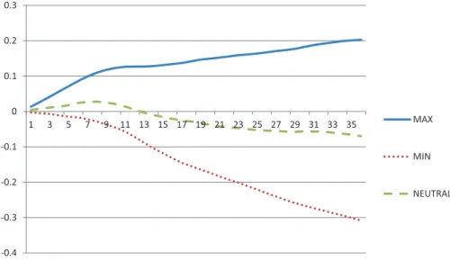
3.1 Raw Return Patterns

Figure 1shows the event time cumulative returns of our portfolios. Although MAX exhibits strong return continuation in the short run, MIN does not. In fact, MIN continues to ex-hibit negative returns in the long run. In other words, the long-run negative returns of MIN do not seem to be a reversal of short-term momentum but instead a continuation of nega-tive performance.

5 Both methods prevent extreme values of ratios affecting mean calculations.

6 Asness (1997);Hong, Lim, and Stein (2000);Lee and Swaminathan (2000);Nagel (2001);Lewellen (2002);Avramov et al. (2007);Sagi and Seasholes (2007);Asness, Moskowitz, and Pedersen (2013); Wahal and Yavuz (2013); andDa, Gurun, and Warachka (2014).

(12)

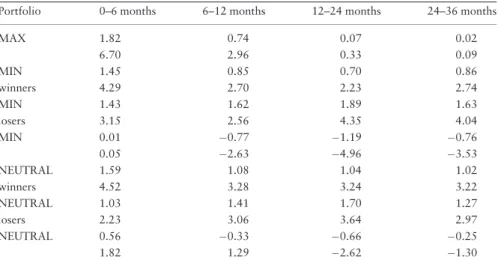
Table V, Panel A displays the average monthly returns of MAX, NEUTRAL, and MIN

portfolios. MAX has an average monthly return of 1.31% (t-statistic¼6.43) in the 0–6

month interval and 0.49% (t-statistic¼2.56) in the 6–12 month holding period, but has no

significant subsequent reversals. MIN has no significant momentum profits in the first 12

months but later displays significant negative returns of0.66%,0.73%, and0.33%

per month in the 6–12, 12–24, and 24–36 month horizons (t-statistics¼ 3.20,4.63, and

2.30, respectively).7_{The NEUTRAL portfolio returns lie in between those of MAX and} MIN and display both momentum and reversals; however even in this case, we find that

these patterns are the result of aggregating returns across different time periods.8_{Table V}_,

Panel B shows that very similar results are obtained by using theJegadeesh and Titman

(1993)methodology, which sorts stocks into deciles based on past returns and invests only in extreme winner and loser stocks.

Overall, when examining raw returns, MAX exhibits momentum but does not exhibit reversal; MIN does not have significant momentum in the first 6 months, but experiences significant negative returns after the first 6 months. In fact, a momentum portfolio that buys all winners and sells all losers except stocks in the MIN portfolio displays significant momentum but no reversal. This implies that reversals arise entirely from the inclusion of securities in MIN, which by construction load negatively on size and book-to-market ratio. Next we explore whether known risk factors explains these findings.

-0.4 -0.3 -0.2 -0.1 0 0.1 0.2 0.3

1 3 5 7 9 11 13 15 17 19 21 23 25 27 29 31 33 35 MAX

MIN

NEUTRAL

Figure 1.The figure plots the average event time cumulative raw returns of MAX, MIN, and NEUTRAL portfolios. These portfolios are described inTable V.

7 We obtain similar patterns when size or book-to-market is individually used as a risk factor in sort-ing stocks into expected return terciles (not reported).

8 Specifically, we examine the returns to MAX, MIN, and NEUTRAL portfolios in two approximately equal subperiods (1965–1987 and 1988–2010). NEUTRAL displays significant momentum but no re-versal in the earlier subperiod, but no momentum and significant rere-versal in the latter subperiod.

(13)

Table V.MAX, MIN, and NEUTRAL portfolio’s raw returns

The table shows the monthly raw returns of MAX, MIN, and NEUTRAL portfolios for the 0–6, 6–

12, 12–24, and 24–36 month holding periods. MAX is a zero investment portfolio, which buys the past winners in the highest expected return tercile and sells the past losers in the lowest

ex-pected return tercile. MIN is a zero investment portfolio, which buys the past winners in the low-est expected return tercile and sells the past losers in the highlow-est expected return tercile.

NEUTRAL include the middle risk winners minus middle risk losers. Stocks are sorted into ex-pected return terciles using stock characteristics of size and book-to-market. We first sort stocks

into terciles using size and book-to-market independently. We classify stocks into the high risk group if the stock is included in the high risk group according to at least one characteristic and

included in at least medium risk by the other characteristic. We classify stocks into the low risk group if the stock is included in the lowest risk group according to at least one characteristic

and included at most in the medium risk by the other characteristic. All other stocks are catego-rized in the medium risk group. Book-to-market is calculated as inFama and French (1992). Size

is the stock market capitalization at the time of portfolio formation. A stock is categorized as winner(loser) if its past 6 month return is higher(lower) than average past 6 month return of all

stocks. A stock’s weight in a portfolio is determined by the absolute difference between stocks’ past 6 month return and the average past 6 month return of all stocks. Weights are normalized

to sum up to 1 within loser and winner sides of portfolios. The sample consists of NYSE, Amex, and Nasdaq stocks between 1965 and 2010. We skip 1 month between the portfolio formation

period and the subsequent holding period. Thet-statistics are reported in the second row and calculated using Newey–West standard errors with 12 months lag.

Portfolio 0–6 months 6–12 months 12–24 months 24–36 months

Panel A:Lo and MacKinlay (1990)methodology

MAX 1.35 0.80 0.60 0.51

winners 4.00 2.57 2.03 1.99

MAX 0.04 0.31 0.58 0.58

losers 0.13 1.05 2.08 2.17

MAX 1.31 0.49 0.02 0.06

6.43 2.56 0.11 0.48

MIN 0.78 0.30 0.21 0.31

winners 2.64 1.08 0.78 1.17

MIN 0.96 0.96 0.94 0.64

losers 2.61 2.78 3.12 2.44

MIN 0.18 0.66 0.73 0.33

0.74 3.20 4.63 2.30

NEUTRAL 1.00 0.53 0.45 0.40

winners 3.13 1.85 1.63 1.56

NEUTRAL 0.59 0.76 0.81 0.49

losers 1.62 2.18 2.63 1.81

NEUTRAL 0.41 0.23 0.36 0.09

2.02 1.31 2.98 1.00

Portfolio 0–6 months 6–12 months 12–24 months 24–36 months Panel B:Jegadeesh and Titman (1993)methodology

MAX 1.99 1.39 1.25 1.32

winners 5.48 3.91 3.70 4.07

MAX 0.17 0.65 1.18 1.29

losers 0.45 1.69 3.17 3.40

(continued)

(14)

3.2 Risk-Adjusted Return Patterns

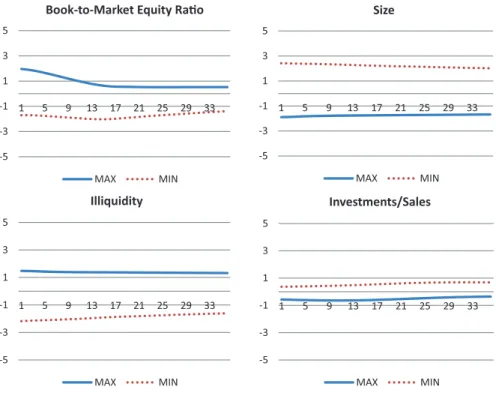
Given that our portfolios differ substantially in terms of size, book-to-market, and other

characteristics summarized inTable IV, we first examine how these differences evolve over

time.Figure 2reports differences in the characteristic quintiles of winner and loser sides of

MAX and MIN. The initial loadings of MAX on size, book-to-market, illiquidity, and asset growth are all associated with higher returns, while the loading on return on assets implies lower returns. Differences in leverage, R&D/sales, dividend growth, and accruals seem small. After the first year, differences between winner and loser sides disappear for book-to-market, return on assets, and asset growth, while differences in size and illiquidity re-main. Unsurprisingly, MIN is the mirror image of MAX at the time of portfolio formation: its initial loadings on size, book-to-market, illiquidity, and asset growth are all associated with lower returns and the loading on return on assets implies higher returns. However, the differences between the winner and loser sides of the MIN portfolio are persistent across all characteristics through time, in contrast to that of MAX portfolio. These differences in portfolio characteristics across size, book-to-market, investment, profitability, and illiquid-ity measures justify controlling for related risk premiums.

Table VIshows MAX, MIN, and NEUTRAL portfolio returns after adjusting for risk using several methods. Given that our portfolios load very differently on size and book-to-market ratio (by construction), we start by using the Fama–French three factor model to

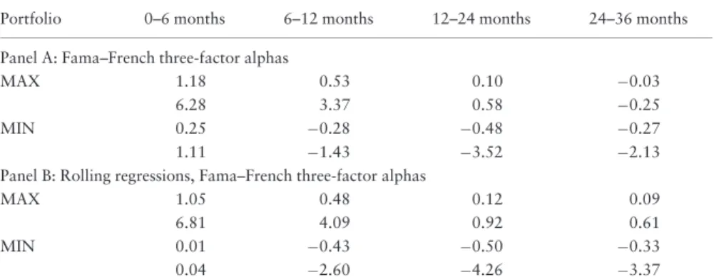
control for risk. Table VI, Panel A shows that MAX has an average monthly return of

1.18% (t-statistic¼6.28) in the 0–6 month holding period, but has no significant

subse-quent reversals. MIN has no significant momentum profits in the first 6–12 months, but

ex-periences significant reversals of0.48% and0.27% per month in the 12–24 and 24–36

month horizons (t-statistics¼ 3.52 and2.13, respectively). Portfolio loadings on factors

are consistent with patterns observed inFigure 2. MAX loads significantly positively on

SMB and HML in the first 6 months with coefficients of 0.48 and 0.30, respectively. These

coefficients decline over the next 12–24 months, to 0.15 and0.04, respectively. MIN

loads significantly negatively on SMB and HML in the first 6 months with coefficients of 0.42 and0.88, respectively. However, the risk loadings for MIN do not decline over Table V.Continued

MAX 1.82 0.74 0.07 0.02

6.70 2.96 0.33 0.09

MIN 1.45 0.85 0.70 0.86

winners 4.29 2.70 2.23 2.74

MIN 1.43 1.62 1.89 1.63

losers 3.15 2.56 4.35 4.04

MIN 0.01 0.77 1.19 0.76

0.05 2.63 4.96 3.53

NEUTRAL 1.59 1.08 1.04 1.02

winners 4.52 3.28 3.24 3.22

NEUTRAL 1.03 1.41 1.70 1.27

losers 2.23 3.06 3.64 2.97

NEUTRAL 0.56 0.33 0.66 0.25

1.82 1.29 2.62 1.30

(15)

time. The persistence in the risk exposures for MIN arises primarily from persistence in the winner portfolio: low risk winners continue to be low risk over time.

We obtain very similar results using the Fama–French three-factor model with 5 year

over-lapping regressions (Table VI, Panel B), to account for the possibility that factor loadings may

change over time. We also consider the possibility that loadings on these factors may be

sensi-tive to the macroeconomy. Specifically, we employ theFerson and Schadt (1996)

method-ology to control for the possibility that loadings on Fama–French three factors may change

with the term premium and default premium.9_{The results, in Panel C of}_{Table VI}_{, indicate}

that the time series of MAX and MIN portfolio excess returns exhibit the same patterns. Given that our portfolios display visible differences across profitability (return on assets) and investment ratios (asset growth and investment/sales), we next examine return patterns

after controlling for theFama and French (2015)five-factor model (Table VI, Panel D). Again,

we obtain very similar patterns; MAX has significant momentum in the 0–6 and 6–12 month periods but exhibits no reversals, while MIN has no momentum but exhibits significant rever-sal between 12–24 and 24–36 months. Neither MIN nor MAX significantly loads on profit-ability. MAX loads significantly positively on the investment factor only in the first 6 months

with a coefficient of 0.61 (t-statistic¼1.93) but not afterwards; this is consistent with the

-5 -3 -1 1 3 5

1 5 9 13 17 21 25 29 33

Book-to-Market Equity Rao

MAX MIN

-5 -3 -1 1 3 5

1 5 9 13 17 21 25 29 33

Size

MAX MIN

-5 -3 -1 1 3 5

1 5 9 13 17 21 25 29 33

Illiquidity

MAX MIN

-5 -3 -1 1 3 5

1 5 9 13 17 21 25 29 33

Investments/Sales

MAX MIN

Figure 2.The figures plot the differences in weighted average of characteristics quintiles of winner and loser portfolios of MAX and MIN during the portfolio holding period between 1 and 36 months. Weights are based on past 6-month returns of stocks relative sample average returns in the same period. Portfolios and characteristics are explained inTable V.

9 Term premium is the difference between 10 and 1 year constant maturity treasury bonds and the de-fault premium is the difference between Moody’s Seasoned Baa minus Aaa Corporate Bond Yield.

(16)

differences in exposure to asset growth converging between winner and loser sides of MAX, as

shown inFigure 2. MIN has a weakly negative coefficient on investment only in the 12–24

month interval (0.28 with at-statistic of1.82). Overall, investment and profitability factors

do not appear to play an important role in explaining the returns patterns that we observe.

We also control for differences in the (il)liquidity of our portfolios using thePastor and

Stambaugh (2003)four-factor model (in Panel E ofTable VI). Neither MAX nor MIN sig-nificantly loads on the liquidity factor at any horizon. Not surprisingly, we obtain similar return patterns after this adjustment for both MAX and MIN. In a later section, we also ex-plore the effect of market level illiquidity on our results.

-5 -3 -1 1 3 5

1 5 9 13 17 21 25 29 33

Return on Assets

MAX MIN

-5 -3 -1 1 3 5

1 5 9 13 17 21 25 29 33

Asset Growth

MAX MIN

-5 -3 -1 1 3 5

1 5 9 13 17 21 25 29 33

Leverage

MAX MIN

-5 -3 -1 1 3 5

1 5 9 13 17 21 25 29 33

R&D/Sales

MAX MIN

-5 -3 -1 1 3 5

1 5 9 13 17 21 25 29 33

Dividend Growth

MAX MIN

-5 -3 -1 1 3 5

1 3 5 7 9 11131517192123252729313335 Accruals

MAX MIN

Figure 2.Continued

(17)

Table VI.Risk-adjusted returns

MAX and MIN portfolios are defined inTable V. The sample consists of NYSE, Amex, and

Nasdaq stocks between 1965 and 2010. We skip 1 month between the portfolio formation period and the subsequent holding period. Thet-statistics are reported in the second row and calculated using Newey–West standard errors with 12 months lag.

Panel A: Fama–French three-factor alphas

MAX 1.18 0.53 0.10 0.03

6.28 3.37 0.58 0.25

MIN 0.25 0.28 0.48 0.27

1.11 1.43 3.52 2.13

Panel B: Rolling regressions, Fama–French three-factor alphas

MAX 1.05 0.48 0.12 0.09

6.81 4.09 0.92 0.61

MIN 0.01 0.43 0.50 0.33

0.04 2.60 4.26 3.37

Panel C: Conditional Fama–French three-factor alphas (term and default premium as conditioning variables)

MAX 1.20 0.61 0.13 0.00

5.88 3.90 0.76 0.03

MIN 0.27 0.26 0.51 0.29

1.19 1.27 3.58 2.33

Panel D: Fama–French five-factor alphas

MAX 1.01 0.59 0.12 0.02

3.84 2.83 0.74 0.13

MIN 0.11 0.23 0.44 0.25

0.35 0.98 2.82 2.05

Panel E: Pastor–Stambaugh four-factor alphas

MAX 1.21 0.53 0.05 0.04

6.19 3.14 0.28 0.30

MIN 0.26 0.27 0.46 0.30

1.04 1.27 3.20 2.28

Panel F: Characteristic-matched returns (33 size and book-to-market sorts)

MAX 0.79 0.16 0.16 0.16

3.79 0.78 1.01 1.12

MIN 0.32 0.29 0.42 0.20

1.60 1.89 3.66 1.93

Panel G: Characteristic-matched returns (1010 size and book-to-market sorts)

MAX 0.74 0.14 0.16 0.16

3.84 0.83 0.80 0.96

MIN 0.24 0.22 0.34 0.03

1.36 1.91 3.90 0.23

Panel H: Carhart four-factor alphas

MAX 0.40 0.21 0.02 0.03

2.29 1.24 0.12 0.24

MIN 0.49 0.45 0.37 0.15

2.95 2.13 2.62 1.20

(18)

In further tests, we control for differences in size and book-to-market characteristics of

our portfolios using an approach similar to that ofDanielet al. (1997). Each month in the

holding period, we assign every security to a matching characteristic portfolio, based on size and book-to-market equity ratios calculated at the time of portfolio formation. Figure 3 presents the cumulative returns of MAX and MIN and their characteristic-matched portfolio cumulative returns with two standard error bands. Cumulative MAX re-turns are significantly higher than characteristic-matched rere-turns for up to 2 years. -0.05

0.00 0.05 0.10 0.15 0.20 0.25 0.30 0.35

1 3 5 7 9 11 13 15 17 19 21 23 25 27 29 31 33 35

MAX

MAX Char.

+ 2SE

- 2SE

-0.35 -0.3 -0.25 -0.2 -0.15 -0.1 -0.05 0

1 3 5 7 9 11 13 15 17 19 21 23 25 27 29 31 33 35

MIN

MIN Char.

+ 2SE

- 2SE

Figure 3.The figure plots the average event time cumulative raw returns of MAX and MIN portfolios and their corresponding characteristics matched portfolios (MAX char and MIN char) with two stand-ard error (SE) bands, which are calculated using Newey–West with lags equal to cumulative return horizon. MAX and MIN portfolios are described inTable V.

(19)

Cumulative MIN returns are slightly higher than characteristic-matched portfolio returns in the first year, but are lower afterwards, always remaining within two standard error bands. The decline in MIN cumulative returns from month 6 to 18 indicates that monthly returns are persistently lower than the corresponding characteristics-matched portfolio monthly returns during this time period. Despite these differences, characteristic-matched returns for MAX are significantly higher than zero for the entire 36-month horizon, while those for MIN are significantly lower than zero for almost the entire time horizon. These results motivate formally evaluating characteristic-adjusted MAX and MIN returns.

In Panel F ofTable VI, we subtract the monthly return of the characteristic-matched

portfolio from the individual security’s return, and re-calculate the characteristic-adjusted MAX and MIN monthly returns. The return differences between these portfolios, especially in the 0–6 month horizon, are significantly reduced, consistent with differences in charac-teristics between the two portfolios being highest in this period. Regardless, characteristic-adjusted MAX continues to have significant momentum in the 0–6 month period and no re-versal afterwards. On the other hand, characteristic-adjusted MIN does not exhibit signifi-cant momentum in the 0–6 month period; instead, it has negative and signifisignifi-cant returns in the 6–12 month and 12–24 months.

In robustness checks, we sort and match on characteristics in a number of different

ways. InTable VI, Panel G we first sort stocks in deciles (instead of terciles) using size and

book-to-market equity, and assign stocks into the high risk category if they are ranked high-est according to one characteristic and are ranked in at least the 7th decile portfolio

accord-ing to the other. We match MAX and MIN stocks with 1010 characteristic-sorted

portfolios and re-calculate characteristic-adjusted returns.10_{Results are qualitatively}

simi-lar across all of these tests.

In summary, after we control for differences in several risk factors and the characteris-tics of MAX and MIN portfolios in various ways, our findings remain. Of course, we are using risk-adjustment methods that are similar to those used elsewhere in the momentum literature—and those results typically show that momentum and reversal patterns survive risk adjustment. As a consequence, it is possible that these controls are inadequate and that the remaining return patterns are due to an omitted risk factor. We consider this possibility in more detail below.

4. Understanding Sources of Momentum

Our evidence to this point indicates that momentum and reversal patterns are separate phenomena—and that forming portfolios at the intersection of characteristics and past re-turns can separate the two. Perhaps more importantly, return continuation seems to be iso-lated in MAX portfolio returns. Examining how these returns are reiso-lated to, or can be explained by, behavioral biases, investor sentiment, liquidity constraints, or macroeco-nomic factors may contribute to our understanding of the sources of momentum.

4.1 Market States

Cooper, Gutierrez, and Hameed (2004)use market states, defined by the lagged returns of the overall market, as a proxy for the behavioral biases that might explain momentum

10 We also obtained similar results after updating the book-to-market equity ratio monthly; this was done by updating market values monthly and updating book values annually.

(20)

returns. In particular, lagged market returns could be a proxy for aggregate investor

confi-dence (Daniel, Hirshleifer, and Subrahmanyam, 1998) or aggregate risk aversion, which

causes greater delayed overreaction and momentum as inHong and Stein (1999).

We follow a similar empirical strategy toCooper, Gutierrez, and Hameed (2004), who

regress cumulative returns of the momentum portfolio on risk factors and then examine the relation between the residuals of this regression and past market returns and its square. We find that lagged market returns positively and significantly explain standard momentum

portfolio profits, confirmingCooper, Gutierrez, and Hameed’s (2004)findings.

y = 0.0097x + 0.0115

-0.4 -0.3 -0.2 -0.1 0 0.1 0.2 0.3

-0.5 0 0.5 1

MAX 6 month returns and past 36 month market returns

y = 0.0272x - 0.0061

-0.4 -0.3 -0.2 -0.1 0 0.1 0.2 0.3 0.4

-0.5 0 0.5 1

MIN 6 month returns and past 36 month market returns

y = -0.0004x + 0.0147

-0.4 -0.3 -0.2 -0.1 0 0.1 0.2 0.3

-3 -2 -1 0 1 2 3

MAX 6 month returns and investor senment index

y = 0.0041x - 0.0011

-0.4 -0.3 -0.2 -0.1 0 0.1 0.2 0.3 0.4

-3 -2 -1 0 1 2 3

MIN 6 month returns and investor senment index

y = 0.0011x + 0.013

-0.4 -0.3 -0.2 -0.1 0 0.1 0.2 0.3

0 0.2 0.4 0.6 0.8

MAX 6 month Returns and Market Illiquidity

y = -0.05x + 0.0014

-0.4 -0.3 -0.2 -0.1 0 0.1 0.2 0.3 0.4

0 0.2 0.4 0.6 0.8

MIN 6 month Returns and Market Illiquidity

Figure 4.The figures plot the monthly returns of the MAX and MIN portfolios in the 0–6 months after portfolio formation on they-axis and other variables on thex-axis. The portfolios are described in

Table V.

(21)

Figure 4plots lagged 36-month returns and future 6-month returns of the MAX and MIN portfolios. Lagged market returns seem to be positively related to the first 6-month re-turn of MIN but not to that of MAX. Confirming this observation, when the dependent variable is the first 6-month return of MIN, the coefficient on lagged market returns is

0.035 with at-statistic of 2.92. However, lagged market returns have no significant

ex-planatory power for the corresponding returns of MAX—which is where momentum prof-its are significant. Moreover, there does not seem to be a connection between the significance of lagged market returns in explaining short-run returns, and the effect of lagged market returns on long-run reversals. Indeed, alphas from this regression (reported inTable VII, Panel A) indicate that MAX and MIN return patterns not only persist, but also appear to be exacerbated when we control for market states.

Overall, lagged market returns do not seem to be an important determinant of MAX portfolio return continuation, and consequently are unlikely to be a fundamental determin-ant of momentum returns.

4.2 Investor Sentiment Index

Baker and Wurgler (2006)construct a sentiment index that predicts future returns of vari-ous zero investment portfolios. If the behavioral biases that can potentially explain momen-tum patterns are correlated with investor sentiment, or if these biases also affect the underlying sentiment proxies discussed above, then we might expect the sentiment index to be correlated with momentum return patterns, and perhaps subsequent reversals as well (Antoniou, Doukas, and Subrahmanyan, 2011).

We test whether the investor sentiment index explains the return patterns that we docu-ment. We measure investor sentiment at the time of portfolio formation by taking a simple average of the sentiment index in the prior 6 months. The sentiment index for a given month is calculated as the average sentiment index of the overlapping momentum port-folios. To control for the sentiment level, we use a regression specification similar to that of Baker and Wurgler’s regression specification (5). Thus, we regress momentum portfolio re-turns on average sentiment in addition to the Fama–French three factors. We find that the investor sentiment index is positively correlated with the returns of the momentum port-folio that invests in all stocks, although this relationship is not significant at the 10% level.

The results indicate that the investor sentiment index is not significant in explaining

re-turns of MAX, but it is (weakly) significant (coefficient of 0.0046 andt-statistics of 1.83) in

explaining the first 6 months returns of the MIN portfolio. These results can also be

inferred fromFigure 4, which plots the subsequent 6-month returns of our portfolios and

the investor sentiment index at the portfolio formation period. Moreover, investor senti-ment is not significant in explaining the returns of any portfolio in the longer horizon 12– 24 and 24–36 month intervals. Thus, there appears to be no link between the portion of momentum explained by the sentiment index and long-run reversals.

Overall, the results in Panel B ofTable VIIindicate that the investor sentiment index is

not important in explaining the time-series patterns that we document, in particular for MAX portfolio returns where momentum profits are evident.

4.3 Market Illiquidity and Arbitrage Constraints

If momentum portfolio returns are a result of arbitrage constraints, then momentum returns

should be higher when aggregate market illiquidity is higher. Recently,Avramov, Cheng, and

(22)

Hameed (2014)consider a possible relation between momentum and market illiquidity, and find, contrary to this intuition, that momentum profits are higher in liquid markets. This is consistent with our finding that MAX has higher returns, despite the fact that constructing MAX involves shorting larger losers which are more liquid compared with MIN portfolio losers. In addition, recall that, despite differences in the (il)liquidity of MAX and MIN,

con-trolling for a liquidity factor does not affect return patterns (seeTable VI, Panel E).

In a separate test, we consider whether variation in market illiquidity is associated with the returns patterns of MAX and MIN portfolios. We measure market illiquidity as the

value-weighted average of each stock’s monthlyAmihud (2002)illiquidity, estimated using

Table VII.Controlling for market factors

The table shows alphas of MAX and MIN portfolios for the 0–6, 6–12, 12–24, and 24–36 month

holding periods after controlling for Fama and French three factors and measures of market sentiment at the time of portfolio formation. Coefficients of past market return and its squared

and investor sentiment index and their significance levels are provided in the text. Panel A re-ports alphas from a regression of portfolio returns on Fama–French three factors and past 36

months market return and its square. We calculate past 36 month return for each month as the equally weighted past 36 month returns of all portfolios that contribute to MAX and MIN returns

for that month. Past 36 months returns are measured at the time of portfolio formation. Panel B reports alphas from a regression of portfolio returns on Fama–French three factors and market

sentiment index fromBaker and Wurgler (2006). We calculate sentiment index for each month as the equally weighted sentiment index of all portfolios that contribute to MAX and MIN

re-turns for that month. Sentiment index is measured at the time of portfolio formation. MAX, MIN portfolios are defined inTable V. The sample consists of NYSE, Amex, and Nasdaq stocks. We

skip 1 month between the portfolio formation period and the subsequent holding period. Thet -statistics are reported in the second row and calculated using Newey–West standard errors

with 12 months lag.

Panel A: Controlling for past market return and market return squared

MAX 1.04 0.66 0.39 0.21

4.84 3.24 2.02 1.34

MIN 0.04 0.33 0.46 0.42

0.14 1.35 3.24 2.58

Panel B: Controlling forBaker and Wurgler (2006)investor sentiment index

MAX 1.30 0.63 0.14 0.01

6.87 4.20 0.79 0.08

MIN 0.34 0.25 0.52 0.29

1.61 1.25 3.62 2.28

Panel C: Controlling for market illiquidity

MAX 1.27 0.39 0.02 0.24

4.79 1.71 0.11 1.32

MIN 0.41 0.31 0.40 0.19

1.31 1.23 2.09 1.13

Panel D: Alpha over returns predicted by Chen, Roll and Ross five factors

MAX 1.00 0.14 0.20 0.14

4.92 0.69 1.12 1.01

MIN 0.34 0.68 0.53 0.24

1.15 2.81 3.21 1.50

(23)

daily data. We use only NYSE/AMEX stocks in the calculation (as inAvramov, Cheng, and Hameed, 2014). The market illiquidity is lagged by 1 month for each momentum portfolio and market illiquidity for a given month is calculated as the average market illiquidity of the overlapping momentum portfolios. We regress momentum portfolio returns on market illiquidity in addition to the Fama–French three factors. These results are presented in Panel C ofTable VII.

For the conventional momentum portfolio, market illiquidity is negatively and

signifi-cantly correlated with momentum portfolio returns, confirming the results ofAvramov,

Cheng, and Hameed (2014). In contrast, both MAX and MIN portfolios returns load nega-tively but insignificantly on market illiquidity in the first 6 months. The negative coeffi-cients arise from the loser side of the portfolios: both MAX and MIN losers (which are shorted) load positively and significantly on market illiquidity. The loadings on market illi-quidity are insignificant for longer horizons, with the exception that MAX has a positive and significant loading in the 24–36 month interval.

Our focus is on the time-series patterns of MAX and MIN alphas, after controlling for market illiquidity. The results in Panel C show that the return patterns of MAX and MIN

remain the same. These results can also be inferred fromFigure 4, which plots the

subse-quent 6-month returns of our portfolios and market illiquidity. In summary, arbitrage con-straints do not seem to explain return continuation in MAX and momentum and reversal patterns continue to be separable.

4.4 Macro-Factors

The findings inAvramov and Chordia (2006)indicate that there may be an undiscovered

risk factor, perhaps related to the business cycle, which has the potential to explain

momen-tum returns. More recently,Liu and Zhang (2008)show that industrial production as a

risk factor can explain a substantial portion of momentum returns. Motivated by these studies we explore whether business cycles affect our findings.

We followLiu and Zhang (2008)and estimate predicted returns using macroeconomic

factors. Specifically, we use the five factors employed inChen, Roll, and Ross (1986)as our

fundamental variables: (log) change in monthly industrial production index, unexpected

in-flation, change in expected inin-flation, term premium, and default premium.11

To estimate premiums associated with macro-variables, we use thirty test portfolios: ten size portfolios, ten book-to-market equity ratio portfolios, and ten momentum portfolios. All portfolios are downloaded from Kenneth French’s website. In the first stage, we use 60-month rolling regressions to estimate factor loadings of the test portfolios on the

macro-fac-tors. In the second stage, we use the methodology inFama–MacBeth (1973)to estimate risk

premiums for the five factors. Next, we use rolling regressions with 60-month windows to es-timate our portfolios’ betas with respect to the calculated risk premiums. Later, betas (based on lagged information) are used together with risk premiums to calculate predicted portfolio

returns. In Panel D ofTable VII, we report the alphas of our portfolios, calculated by

sub-tracting predicted returns from realized returns. We find that MAX returns are reduced by 30 basis points in the first 6 months and by 10–25 basis points in subsequent intervals. MIN re-turns are also reduced by 15 basis points in the first 6 months, followed by an increase of about 20 basis points in the interval between 12 and 24 months. Our findings are consistent

11 We download factors from Laura Liu’s website, where detailed definitions of these variables are provided.

(24)

with macro-factors explaining a non-trivial fraction of initial momentum returns. However, MAX intermediate term profits remain significant after controlling for macro-factors.

4.5 An Omitted Risk Factor

The results presented inTable VI indicate that the differences in characteristic-adjusted

MAX and MIN returns are positive, and relatively stable, declining monotonically over the 3-year horizon that we examine (averaging 0.47%, 0.45%, 0.26%, and 0.04% per month, in months 0–6, 6–12, 12–24, and 24–36, respectively). In fact, these patterns are similar to the difference between MAX and MIN alphas with respect to Fama–French three factors, which also decline slowly over time (with alphas at 0.93%, 0.81%, 0.38%, and 0.24% per month in months 0–6, 6–12, 12–24, and 24–36, respectively).

It is difficult to ascribe the different behavior of characteristic-adjusted MAX and MIN re-turns to either momentum, or characteristics, alone. First, considered as momentum

strat-egies, MAX and MIN have similar loadings on the momentum factor12_{and the results}

remain similar after controlling for the Carhart four-factor model (Table VI, Panel H).

Second, since the results inTable VI, Panels F and G are characteristic-adjusted returns, it

seems unlikely that the differences are due to market capitalization, or book-to-market effects alone. The results may indicate an omitted risk factor beyond the characteristics we control for or that their interactions with past returns act as a proxy for the omitted risk factor.

5. Conclusion

We present evidence that short-term momentum and long-run reversals are separate phe-nomena. Stocks that display momentum in the first 6 months do not display significant re-versal in the long run. In contrast, contrarian stocks in the first 6 months display significant reversal in the 12–24 month period. Merging these separate subgroups of securities makes momentum and reversal patterns appear to be linked.

We show that it is possible to identify portfolios of stocks that have momentum from those that experience reversals at the time of portfolio formation, using size and book-to-market equity ratio as characteristics that predict returns. A portfolio (MAX) that buys small, high book-to-market stocks and sells large market capitalization, high book-to-mar-ket stocks displays significant momentum but no reversal. In contrast, a portfolio (MIN) that buys large, high book-to-market stocks and shorts small, low book-to-market stocks has no momentum, but exhibits significant reversal. These returns patterns are not ex-plained by differences in loading on known risk factors or after adjusting for characteris-tics-matched returns using various methods. In all of the tests, it appears that momentum and reversal patterns are separate and distinct.

To better understand sources of momentum, we analyze whether these return patterns are explained by market level investor sentiment, past market returns, market illiquidity, or macro-variables. We find that MAX portfolio returns are potentially easier to arbitrage away (since shorting less illiquid and larger stocks should be cheaper) but display larger re-turn continuations, which do not vary with investor sentiment, past market rere-turns, or mar-ket illiquidity. Macroeconomic variables explain a portion of profits, but the residual profits for MAX remain positive and large.

12 The coefficient of the momentum factor is 0.83 for the MAX portfolio and 0.78 for the MIN portfolio and highly significant for both in explaining the first 6-month returns.