R E S E A R C H
Open Access
Controlling the dynamic range of a
Josephson parametric amplifier
Christopher Eichler
*and Andreas Wallraff
*Correspondence:
Department of Physics, ETH Zürich, Zürich, 8093, Switzerland
Abstract
One of the central challenges in the development of parametric amplifiers is the control of the dynamic range relative to its gain and bandwidth, which typically limits quantum limited amplification to signals which contain only a few photons per inverse bandwidth. Here, we discuss the control of the dynamic range of Josephson parametric amplifiers by using Josephson junction arrays. We discuss gain,
bandwidth, noise, and dynamic range properties of both a transmission line and a lumped element based parametric amplifier. Based on these investigations we derive useful design criteria, which may find broad application in the development of practical parametric amplifiers.
1 Introduction
Due to the rapidly evolving field of quantum optics and information processing with su-perconducting circuits the interest in low-noise amplifiers has dramatically increased in the past five years and has lead to a body of dedicated research on Josephson junction based amplifiers [–]. The most successful quantum limited detectors which have so far been realized in the microwave frequency range are based on the principle of parametric amplification [–]. Josephson parametric amplifiers (JPAs) have not only been used to generate squeezed radiation [, , –], but moreover enabled the realization of quan-tum feedback and post-selection based experiments [–], the efficient displacement measurement of nanomechanical oscillators [] and the exploration of higher order pho-ton field correlations [, ].
While JPAs have been demonstrated to operate close to the quantum limit, their
perfor-mance is to date mostly limited by their relatively small dynamic range,i.e.the saturation
of the gain for large input signals. Here, we discuss the control of the dynamic range by making use of Josephson junctions arrays in the parametric amplifier circuit, which we have already employed in recent experiments [, ]. After reviewing the principles of parametric amplification we discuss bandwidth and noise constraints in dependence on the circuit design, based on which we derive simple strategies for optimized circuit design.
2 Principles of parametric amplification
2.1 Parametric processes at microwave frequencies
In quantum optics the wordparametricis used for processes in which a nonlinear
re-fractive medium is employed for mixing different frequency components of light. Such processes are parametric in the sense that a coherent pump field, applied to a nonlinear
medium, modulates its refractive index, which appears as aparameterin a semi-classical treatement. This time-varying parameter is affecting modes with frequencies detuned from the frequency of the pump field and can stimulate their population with photons. The energy for creating these photons is provided by the pump field.
The refractive index in optics is equivalent to the impedance of electrical circuits. In order to realize parametric processes at microwave frequencies we therefore modulate an effective impedance. This is achieved by varying the parameters of either a capaci-tive or an induccapaci-tive element in time. Although there have been early proposals for fast time-varying capacitances [], it now is considered to be more convenient to make use
of dissipationless Josephson junctions for this purpose. In a regime in which the currentI
flowing through a Josephson junction is much smaller than its critical currentIC≡eEJ/
its associated inductance is approximatelyL≈LJ( +(I(t)/IC)). Applying anACcurrent
through the junction using appropriate microwave drive fields therefore leads to the
de-sired time-varying impedance. Because of the proportionality of the inductanceLto the
square of the currentI(t), such a drive results in a four-wave mixing process []. The effective impedance can alternatively be modulated by varying the magnetic flux threading a superconducting quantum interference device (SQUID) loop [] such that
the effective inductance is approximately modulated proportionally to the AC currentI(t)
flowing in the loop,L≈LJ( +I(t)/I). The quantityIin this expression depends on the DC flux bias point of the SQUID loop. Since the relation between current and inductance is in this case linear, the magnetic flux drive results in a three-wave mixing process [].
In order to enhance parametric amplification in a well-controlled frequency band while suppressing it for frequencies out of this band, the modulated Josephson inductance is frequently integrated into a microwave frequency resonator. This is the simplest way to control the band in which parametric amplification occurs. A number of variations of this basic idea are now explored. The circuit design has recently been modified to achieve a spatial separation of signal and idler modes [, , –] and to build traveling wave amplifiers, in which a field is amplified while propagating in forward direction coaxially with a pump field [, ]. Various drive mechanisms ranging from single and double pumps [] to magnetic flux drives [, , ] have been explored. Being aware of this variety of possible approaches, we focus here on a single mode (degenerate) parametric amplifier driven with one pump tone close to its resonance frequency.
2.2 Circuit QED implementation of a parametric amplifier
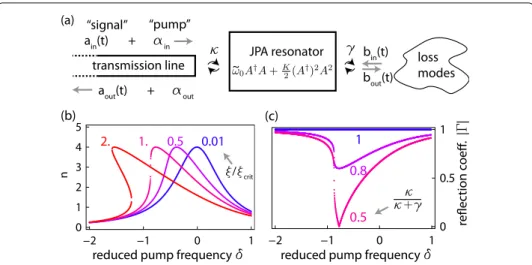
The JPA essentially is a weakly nonlinear oscillator, in which the nonlinearity is provided by Josephon tunnel junctions. In practice, this is typically realized either as a transmission line resonator shunted by a SQUID [, , ], see Figure (a), or as a lumped element nonlinear oscillator []. The use of a SQUID instead of single tunnel junction guarantees tunability of the resonance frequency. Since resonator-based parametric amplifiers pro-vide amplification in a narrow band only, tunability is highly desirable to match the band of amplification with the frequency of the signal to be amplified.
The relevant part of the Hamiltonian which describes the parametric amplifier consid-ered here can be written as
HJPA=ω˜A†A+
K
Figure 1 Schematic and operation of the parametric amplifier.(a) Circuit diagram of a transmission line resonator based parametric amplifier. The resonator is coupled with capacitanceCκto a transmission line where input and output modes are spatially separated using a circulator. A 20 dB directional coupler between theλ/4-resonator and the circulator is used to apply the pump field required for modulating the SQUID inductance. The second port of the directional coupler can be used to interferometrically cancel out the pump tone reflected from the sample. (b) Phase of the reflected probe signalvs.drive power for two characteristic drive frequencies below (blue) and above (red) the bifurcation threshold. (c) Illustration of the nonlinear oscillator response in the quadrature plane. The blue circle represents various input fieldsαinclose to the one indicated by the gray circle in (b). Due to the nonlinear response of the resonator they are transformed into output fieldsαoutindicated by the red ellipse.
whereAlabels the annihilation operator of the intra-resonator field. Expressions for the
resonance frequencyω˜/πand the effective Kerr nonlinearityKare derived in Section
based on the full circuit model. In the following section we analytically study the dynam-ics of this system using the input-output formalism. Before presenting the mathematical derivations, we qualitatively describe different dynamical regimes of this nonlinear oscil-lator and explain the mechanism which leads to amplification.
If we assume for the moment that the JPA has no internal losses, all the incident power is
reflected from the resonator and the classical response (i.e.reflection coefficient) is
com-pletely specified by the phaseϕof the reflected field. In contrast to a linear system, whereϕ
only depends on the frequencyω/π, it also depends on the power of the probe field in the
case of a nonlinear oscillator. In Figure (b), the theoretically expected value ofϕis
plot-ted as a function of the probe amplitude for two characteristic drive frequencies. While the phase is constant for low drive powers (quasi-linear response), the phase changes sig-nificantly for increased drive power. Depending on the probe frequency we either find a bistable regime where two stable solutions exist [, ] or a regime where the phase has a unique solution (red and blue data sets in Figure (b)). In both cases the phase significantly depends on the input power. The bistable response can for example be used to realize a bifurcation amplifier [, ] and for nonlinear dispersive readout [], which has been intensely studied in the context of circuit QED.
Since we are particularly interested inlinearamplification the following discussion is
Figure 2 Input-output model.(a) Schematic of the input-output model used for calculating the response of the parametric amplifier in the presence of additional loss modes. (b) Normalized pump field photon numbernin the resonator as a function of reduced pump frequencyδfor effective drive strengths ξ/ξcrit= 0.01, 0.5, 1, 2, whereξcrit= –1/√27. (c) Absolute value of the reflection coefficient||for different coupling ratiosκ/(κ+γ) = 1, 0.8, 0.5.
imagine that the device is constantly driven at a frequency and power at which the
re-flected phaseϕ depends sensitively on power (see gray circle in Figure (b)), the system
will strongly react to small perturbations. Such perturbations, which could be caused by an additional small signal field for example, are therefore translated into a large change of the output field.
We illustrate this process leading to amplification by plotting the resonator response
for input fieldsαin with slightly varying amplitude and phase. In Figure (c) we indicate
the input fields by a blue circle around the mean value (arrow). The small differences in
amplitude of the input field translate into large changes inϕof the output fieldαout(red
ellipse). If we interpret the arrow in Figure (c) as a constant pump field and its difference to the points on the blue circle as an additional signal, the signal is either amplified or deamplified depending on its phase relative to the pump.
The mechanism of amplification can thus be understood intuitively by considering the nonlinear response to a monochromatic drive field. In order to characterize the exact be-havior of input fields with finite bandwidth we analyze the response in more detail below.
3 Input-output relations for the parametric amplifier 3.1 Classical nonlinear response
Here, we employ the input-output formalism [, ] to calculate the nonlinear resonator response discussed qualitatively in the previous section. The derivation presented here is inspired by Ref. []. A schematic of the input-output model is shown in Figure . The
nonlinear resonator is coupled with rateκto a transmission line, through which the pump
and signal fields propagate. Based on this model and the Hamiltonian in Eq. () we obtain the following equation of motion for the intra-resonator field
˙
A= –iω˜A–iKA†AA–
κ+γ
A+
√
In addition to the coupling to transmission line modesAin(t) with rateκ we account for
potential radiation loss mechanisms by introducing the coupling to modesbin(t) with loss
rateγ, compare Figure (a). A boundary condition equivalent to
Aout(t) =
√
κA(t) –Ain(t), ()
also holds for the loss modes. When operating the device as a parametric amplifier, the
input fieldAin is typically a sum of a strong coherent pump field and an additional weak
signal field. Since this signal carries at least the vacuum noise, it is treated as a quantum field. In this formalism this particular situation is accounted for by decomposing each field mode into a sum of a classical part and a quantum part
Ain(t) =
ain(t) +αin
e–iωpt, Aout(t) =
aout(t) +αout
e–iωpt, ()
A(t) =a(t) +αe–iωpt,
whereα,αin,αoutrepresent the classical parts of the field which are associated with the
pump, whilea,ain,aoutaccount for the quantum signal fields. Since allα’s are complex
numbers the modesasatisfy the same bosonic commutation relations as modesAdo. By
multiplying the field modes defined in Eq. () with the additional exponential factore–iωpt,
one works in a frame rotating at the pump frequencyωp. The strategy is to first solve the
classical response for the pump fieldαexactly and then linearize the equation of motion
for the weak quantum fieldain the presence of the pump. Finally, we derive a scattering
relation between input modesainand reflected modesaout.
The steady state solution for the coherent pump field is determined by
i(ω˜–ωp) +
κ+γ
α+iKαα∗=√καin, ()
which follows immediately by substituting Eq. () into Eq. () and collecting only the c-number terms. By multiplying both sides with their complex conjugate we get to the equa-tion
κ
(κ+γ)|αin| =
ωp–ω˜
κ+γ
+
|α|–(ωp–ω˜)K (κ+γ) |α|
+
K
κ+γ
|α|, ()
which determines the average number of pump photons|α|in the resonator. Eq. ()
re-duces to
=
δ+
n– δξn+ξn, ()
by defining the scale invariant quantities
δ≡ωp–ω˜
κ+γ , α˜in≡
√
καin
κ+γ , ξ≡
| ˜αin|K
κ+γ , n≡
|α|
| ˜αin|
. ()
δis the detuning between pump and resonator frequency in units of the total resonator
and nonlinearity, also expressed in dimensionless units. Finally,nis the mean number of pump photons in the resonator relative to the incident pump power. As an important consequence, we notice from Eq. () that only the product of drive power and nonlinearity determines the dynamics but not each quantity itself. Therefore, a small nonlinearity can at least in principle be compensated by increasing the drive power. Properties such as the gain-bandwidth product are therefore independent of the strength of the nonlinearity as long as the pump power is much larger than the power of amplified fluctuations.
Further-more, the solutions of Eq. () for negativeξ values are identical to those for positiveξ up
to a sign change inδ. Sinceξ is negative for the Josephson parametric amplifier, we focus
on this particular case.
Equation () is a cubic equation innand can therefore be solved analytically. We do not
present the lengthy solutions here explicitly, but assume in the following that we have an explicit analytical expression fornin terms ofδandξ. In Figure (b) we plotnfor various parametersξ as a function ofδ. At the critical valueξcrit= –/
√
the derivative∂n/∂δ
diverges and thus the response of the parametric amplifier becomes extremely sensitive to small changes. For even stronger effective drive powersξ/ξcrit> the cubic Eq. () has three real solutions. The solutions for the high and low photon numbers are stable, while the intermediate one is unstable. The system bifurcates in this regime as mentioned earlier.
The critical detuning below which the system becomes bistable isδcrit= –
√
/. The crit-ical point (ξcrit,δcrit) is the one at which both∂δ/∂nand∂δ/∂nvanish. In scale invariant
units the maximal value ofnis , which is reached at the detuningδ= ξ.
Experimentally, the system parameters are characterized by measuring the complex
re-flection coefficient≡αout/αin. Based on the input-output relationαout=
√
κα–αinand Eq. () we evaluate this reflection coefficient as
= κ
κ+γ
–iδ+iξn
– . ()
In Figure (c) we plot the absolute value of the reflection coefficient atξ=ξcritfor various
loss ratesγ. For vanishing lossesγ = all the incident drive power is reflected from the
device and||= . Note that also in this case the resonance is clearly visible in the phase
of the reflected signal (not shown here). When the loss rate γ becomes similar to the
external coupling rateκpart of the radiation is dissipated into the loss modes. In the case
of critical couplingγ =κ all the coherent power is transmitted into the loss modes at
resonance. This is equivalent to the case of a symmetrically coupledλ/ resonator, for
which the transmission coefficient is one at resonance [].
3.2 Linearized response for weak (quantum) signal fields
Under the assumption that the photon flux associated with the signal a†inainis much
smaller than the photon flux of the pump field|αin|, we can drop terms such asKa†aα, be-cause they are small compared to the leading termsKa†αandKa|α|. By neglecting these
terms we obtain a linearized equation of motion forain the presence of the pump field.
In order to preserve the validity of this approximation even for larger input signals, the
amplitudeαof the pump field needs to be increased. Experimentally, this can be achieved
Substituting Eq. () into Eq. () and keeping only terms which are linear inaone finds
˙ a(t) =i
ωp–ω˜– K|α|+i
κ+γ
a(t) –iKαa†(t) +√κain(t) +√γbin(t). ()
Since Eq. () is linear, we can solve it by decomposing all modes into their Fourier com-ponents
a(t)≡κ√+γ π
∞
–∞de
–i(κ+γ)ta
()
and equivalently forain,andbin,. Note that the detuningbetween signal frequencies
and the pump frequency, is expressed here in units of the linewidthκ+γ. Substituting the
Fourier decompositions into Eq. () and comparing the coefficients of different harmon-ics, results in
=
i(δ– ξn+) –
a–iξneiφa†–+c˜in,, ()
where ˜cin,≡(√κain,+√γbin,)/(κ+γ) is the sum of all field modes incident on the
resonator. Furthermore, in Eq. ()φis the phase of the intra-resonator pump field, defined
byα=|α|eiφ. The fact that Eq. () couples modesa anda
†
–can be interpreted as a wave
mixing process. In order to expressain terms of the input fieldscin,, Eq. () is rewritten as a matrix equation
˜ cin,
˜ c†in,–
=
i(–δ+ ξn–) + iξneiφ –iξne–iφ i(δ– ξn–) +
a
a†–
. ()
By inverting the matrix on the right hand side, the quantum part of the intra-resonator fieldais expressed in terms of the incoming field˜cin,
a=
i(δ– ξn–) + (i–λ–)(i–λ+)˜
cin,+
–iξneiφ (i–λ–)(i–λ+)˜
c†in,– ()
withλ±=± (ξn)– (δ– ξn). Using Eq. (), the final transformation between input and output modes is
aout, = gS,ain,+gI,a †
in,–+
γ
κ(gS,+ )bin,+
γ κgI,b
†
in,– (a)
γ/κ→
= gS,ain,+gI,a †
in,–, (b)
with
gS,= – +
κ κ+γ
i(δ– ξn–) + (i–λ–)(i–λ+)
()
and
gI,=
κ κ+γ
–iξneiφ (i–λ–)(i–λ+)
Figure 3 Parametric amplifier gain.(a)G=|gS,|2vs.pump tone detuningδand drive strengthξat zero signal detuningand forκ=γ. For increasing drive strengthξthe detuning for maximum gain is indicated by the dashed white line. A cut through the data for the highest valueξ= 0.98ξcritis shown as the solid white line in the bottom part. (b) Gain as a function of signal detuningfor the indicated drives strengthsξ/ξcrit and optimal pump detuning. The exact gain curves (solid lines) are well approximated by Lorentzian lines (black dashed lines).
Eq. (b) is the central result of this calculation. The output field at detuningfrom the
pump frequency is a sum of the input fields at frequencies and –multiplied with
the signal gain factorgS,and the idler gain factorgI,, respectively. The additional noise
contributions introduced via the loss modesbin,vanish in the limitγ/κ→. In the ideal
caseγ = , the coefficientsgS,andgI,satisfy the relation
G≡ |gS,|=|gI,|+ ()
and Eq. (b) is identical to a two-mode squeezing transformation [, ] with gainG.
The two-mode squeezing transformation describes a linear amplifier in its minimal form (compare Ref. []), of which we discuss characteristic properties in the following section.
3.3 Gain, bandwidth, noise and dynamic range
For simplicity we consider the case of no lossesγ = , for which the parametric amplifier
response is described by Eq. (b). An incoming signal at detuningis thus amplified by
the power gainG=|gS,| and mixed with the frequency components at the opposite
detuning from the pump. Characteristic properties of the parametric amplifier, such as
the maximal gain and the bandwidth, are thus encoded in the quantitygS,as a function
of pump-resonator detuningδ, effective drive strengthξand detuning between signal and
pump.
In Figure (a) we plot the gainGfor zero signal detuning = as a function ofδ
andξ. We find that the maximal gain increases with increasing drive strengthξ while
the optimal value forδ at which this gain is reached, shifts approximately linearly with
increasingξ. The optimal values forδare indicated as a dashed white line in Figure (a).
Mathematically, the gain diverges whenξ approaches the critical valueξcrit. In practice,
the gain is limited to finite values due to the breakdown of the stiff pump approximation (see discussion below).
By changing the pump parametersξandδwe can adjust the gainGto a desirable value,
presence of finite internal lossesγ > . Once the pump parameters are fixed we character-ize the bandwidth of the amplifier by analyzing the gain as a function of the signal detun-ing. In Figure (b) we plot the gain as a function offor the indicated values ofξ/ξcrit
and the corresponding optimal pump detuningsδ(compare dashed white line in (a)). The
gain curves are well approximated by Lorentzian lines as indicated by the dashed black lines in Figure (b). When the gain is increased, the band of amplification becomes
nar-rower. This is quantitatively expressed by the gain-bandwidth relation√GB≈, whereB
is the detuningfor which the gain reaches half of its maximal value. This gain-bandwidth
relation follows from the Lorentzian approximation of the gain curves shown as black
dashed lines in Figure (b)) and holds for gain values above a few dB. Remember that
is defined in units of the resonator linewidthκ+γ, which means that the amplifier
band-width equals approximately the resonator lineband-width divided by the square root of the gain. When operating the JPA, we also have to understand its behavior in terms of added
noise. In the ideal case with zero loss rate (γ = ), the input-output relation of the
para-metric amplifier in Eq. (b) has the minimal form of a scattering mode amplifier []. The amplification process reaches the vacuum limit as long as the input modes are cooled into
the vacuum. In practice, however, the device may have finite lossγ which increases the
ef-fectively added noise by a factor of (κ+γ)/κ. This is due to the additional amplified noise,
which originates from the modesbin,and contributes to the output fieldaout,(compare
Eq. (a)). Another potential source of noise is related to the stability of the resonance fre-quency of the parametric amplifier. Magnetic flux noise in the SQUID loop may lead to a fluctuating resonance frequency and thus a fluctuating effective gain.
In the derivation made in the previous sections we have assumed that the solution of the classical drive field is unaffected by the presence of additional signal and quantum fluctu-ations at the input. This is known as the stiff pump approximation [], which assumes that the pump power at the output is equal to the pump power at the input of the JPA. This is of course an approximation, since the pump field provides the energy which is neces-sary for amplifying the input signal. The stiff pump approximation is valid as long as the pump power is significantly larger than the total output power of all amplified (quantum) signal and vacuum fields. In order to quantitatively analyze the pump depletion due to the
presence of amplified fields we add the terms iKa†aα andiKaα∗ to the left hand
side of Eq. () and solve Eq. () and Eq. () self-consistently. This mean-field approach is similar to the one used in Ref. []. For our calculation we model the incoming signal
field, which is to be amplified, as white noise with average photon numbernthper unit
time and bandwidth. Based on this model we find that the gain decreases when the signal
strength exceeds a certain value, see Figure (a). The number of input photonsnthat which
this happens becomes smaller with decreasing ratioκ/|K|. This is expected because the
pump power close to the bifurcation point is proportional toκ/|K|and provides the
en-ergy required for amplification. For small valuesκ/|K|the gain is reduced even fornth= due to the amplification of vacuum fluctuations (see blue data points in Figure (a)). As a
measure of the dynamic range we specify the dB compression point of the JPA,i.e.the
valuen dB of input photonsnthat which the JPA gainGdecreases by dB compared to
the stiff pump approximated gain value. As shown in Figure (b), the dB compression point increases proportionally toκ/|K|in the limit ofn dB. The presence of constant
vacuum fluctuations leads to a gain compression by more than dB even fornth= when
Figure 4 Dynamic range of the JPA.(a) GainG0as a function of the photon numbernthof the input signal
field for the three indicated ratiosκ/|K|. (b) 1 dB compression point as a function ofκ/|K|for various gain valuesG0.
powerPp=ωp|αin|with the power of amplified signal and vacuum fields
Pout
γ=
= ωpκ(nth+ )
d
π(G– ). ()
Making use of the gain-bandwidth relation we find the following scaling of the ratio be-tween the two powers
Pout
Pp ∝
(nth+ )|
K|
κ G. ()
The results shown in Figure (b) together with Eq. () indicate that the validity of the
stiff pump approximation is essentially determined by the ratioPout/Pp. The calculations
furthermore show that the dynamic range can be increased by reducing the ratio|K|/κ
of the JPA, which seems to be the case also for flux driven parametric amplifiers []. In Section we discuss how to achieve small nonlinearities by making use of multiple SQUIDs connected in series.
4 Effective system parameters from distributed circuit model
In the previous section we have analyzed the model of a nonlinear resonator with
reso-nance frequencyω˜, Kerr nonlinearityKand decay rateκ. Here, we explicitly derive this
effective Hamiltonian from the full circuit model of aλ/ - transmission line resonator,
which is terminated by a SQUID loop at the short-circuited end and coupled capacitively to a transmission line, see Figure (a). These calculations allow us to determineω˜,K,κ from the distributed circuit parameters and give insight into potential limitations of the effective model. We also compare the obtained parameter relations with those of a lumped element parametric amplifier.
4.1 Resonator mode structure in the linear regime
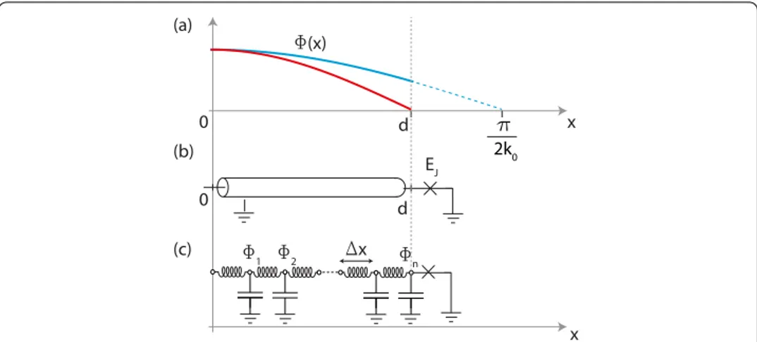
Figure 5 Circuit model.(a) Distribution of the magnetic flux field(x) along theλ/4-resonator for the fundamental resonator modej= 0, without (red) and with (blue) a Jospehson junction. The additional Josephson inductance changes the boundary condition such that neither the current nor the voltage is zero at positionx=d. The resulting increase in the effective wavelengthπ/(2k0) is indicated by the dashed blue
line. (b) Transmission line resonator of lengthdwith a Josephson junction at the grounded end. (c) Lumped element representation with indicated discretized magnetic flux fieldjas used in Eq.().
The total Lagrangian of the system in the magnetic flux field(x) has a transmission
line part and a term which describes the SQUID at positionx=d(Figure ).
L=
d
dx
c
∂t(x)
–
l
∂x(x)
+EJcos
(d)
ϕ
, ()
with the reduced flux quantumϕ=/e. Since we work in a limit in which the plasma
frequency of the SQUID is much larger than the resonance frequencies of interest, we neglect the self-capacitance of the SQUID. Note that Ref. [] provides a detailed study of the effect of the self-capacitance in various parameter regimes. We furthermore describe
the SQUID as a single junction with tunable effective Josephson energyEJ.
We first investigate the linear regime of the system, in which the cosine potential of the SQUID is approximated as a quadratic potential.
EJcos
(d)
ϕ
≈const –
(d)
ϕ
. ()
Due to the spatial derivative in the Lagrangian in Eq. () all local fields in the chain are coupled to their nearest neighbors and the normal mode structure is found by solving the Euler-Lagrange equation∂t(δL/δ˙) –δL/δ= of the transmission line resonator. This
results in the wave equation
v∂x(x) –∂t(x) = , ()
with the phase velocityv= /√cl, of which the general solution can be written as a sum of
normal modes
(x) =
∞
j=
The valid wavevectorskjare determined by the boundary conditions at the two ends of the
λ/ transmission line. The open end atx= requires that the current∂x(x)/lvanishes,
which is implicitly satisfied by choosing the cosine ansatz in Eq. (). On the shorted end the boundary condition is modified by the presence of the Josephson junction. In order to determine this boundary condition, we evaluate the Euler-Lagrange equation at position
x=d. For this purpose it is convenient to write the Lagrangian in a discretized form, see
Figure (c) and compare Ref. []:
L= lim
n→∞ n
j=
x
c
(∂tj)
–
l
(j–j–)
x
–
EJ
n
ϕ
, ()
where n=(x=d) andx=d/n. Evaluating ∂t(∂L/∂˙n) –∂L/∂n= leads to the
equation
l∂x(d) +EJ
(d)
ϕ = . ()
Substituting the ansatz () into Eq. () and comparing the resulting coefficients of the
independent variablesφj, results in the transcendental equation
kjdtan(kjd) =ld
EJ
ϕ
≡ld LJ
. ()
Here, we have defined the Josephson inductanceLJ=ϕ/EJ. The infinite set of solutionskj
of this equation determines the normal modes structure of the system in the linear regime.
In the limit in which the SQUID inductanceLJvanishes, Eq. () is solved by the poles of
tan(kjd), and we recover the normal modes of theλ/ resonator
kj()d=π
( + j) withj∈ {, , , , . . .}. ()
As a first order correction to this result in the limit ofLJ/ld, we expand Eq. () to
first order in (kj()–kj)dand findkjLJ/ld= (k()–kj) or equivalently
kj≈
k()j
+LJ/ld
. ()
For the fundamental mode withj= this linearized approximation is typically accurate
even for inductance ratios up toLJ/ld≈., whereas for the higher harmonic modes the
linearized equation breaks down for much smaller values ofLJ/ld. A comparison between
the exact solution based on Eq. () and the approximate solution in Eq. () is shown in Figure for the first three resonant modes. When higher harmonics are expected to be relevant one should solve Eq. () numerically in order to determine the exact wave numberskj.
4.2 Kerr nonlinear terms and effective Hamiltonian
Figure 6 Resonance frequencies of the first three modes as a function of Josephson energy.The solid line results from the exact numerical solution of Eq.()while the dashed line shows the linearized solution in Eq.(). The bare resonance frequency is chosen to be 7 GHz and the impedance of the transmission line resonator 50.
SQUID. For the purposes of parametric amplification the phase drop across the junction is desired to be small,n/ϕ< ,i.e.the current flowing through the Josephson junction is small compared to its critical current. We can therefore expand the SQUID cosine po-tential and take into account only the first non-quadratic correction
EJcos
n
ϕ
= const –
EJ
n
ϕ
+
EJ
n
ϕ
+· · ·. ()
In Section we discuss under which circumstances such an approximation may break down. Substituting the normal mode decomposition Eq. () into the Taylor expansion of the Lagrangian results in
L=
∞
i= ˙
φiCiφ˙i–φiL–i φi
+
∞
j,i,k,l=
Nijklφiφjφkφl ()
with the effective capacitances and inductances []
Ci=c
d
dxcos(kix) =
cd
+sin(kid) kid
,
L–i = L–J cos(kid) +
ki l
d
dxsin(kix) ()
Eq. () = (kid)
ld
+sin(kid) kid
,
and the nonlinearity coefficients
Nijkl=
EJϕ
–
m∈{i,j,k,l}
cos(kmd). ()
As expected the linear part of the Lagrangian is diagonal in the normal mode basis. It
describes a set of uncoupledLCoscillators for which the effective resonance frequencies
coincide with the product of phase velocity and wave vectorωj=kjv= / LjCj.
tak-ing only self-interactions and two-mode interactions into account, results in the Hamilto-nian
H=
∞
i=
qiCi–qi+φiL–i φi
–
∞
j=i
Niijjφiφj –
∞
i
Niiiiφi. ()
In a quantum regime qi andφi are operators which satisfy the commutation relation
[φj,qk] =δkj/iand it is convenient to write the Hamiltonian in terms of normal mode
annihilation and creation operators []
φj=iφzpf,j
a†j –aj
, qj=qzpf,j
aj+a†j
()
withqzpf,i=
√
ωiCi/ andφzpf,i=
√
/ωiCi. The abbreviation zpf stands for zero point
fluctuations. Performing a rotating wave approximation (i.e.removing all terms with an
unequal number of creation and annihilation operators), and neglecting the small photon
number independent frequency shifts due to the nonlinear terms (i.e.Lamb shifts) we
arrive at
H=
∞
i=
ωia
†
iai+
Kii
a
†
ia
†
iaiai+
∞
j=i
Kija
†
iaia
†
jaj ()
with
Kij= –
EJ φzpf ϕ
cos(kid)cos(kjd). ()
The quantityK=Kis the Kerr nonlinearity of the fundamental mode, which is used for
the parametric amplification process. The terms proportional toKijwith unequali=jare
cross Kerr interaction terms which couple different modes to each other. Such an interac-tion can for example be used for counting the number of photons in one mode by probing another one with a coherent field [–], similarly to a dispersive qubit measurement. Note that the values resulting from Eq. () are divided by the square of the number of SQUIDs, if an array is used instead of a single SQUID, as discussed in the following sec-tion.
4.3 Decay rate and resonance frequency correction for lowQresonators
Since the parametric amplifier bandwidth is proportional to the decay rateκ, typical
de-vices are designed to have a low external quality factor, which is achieved by increasing the
coupling capacitanceCκbetween transmission line and resonator (Figure ). The coupling
of an oscillator to the environment shifts its resonance frequencyωj→ ˜ωj[], which can
be significant if the coupling rate is large. When designing parametric amplifier devices, it is therefore necessary to take these shifts into account. Based on the effective inductance and capacitances calculated in Eq. () we find
˜
ωj ≈ ω
j
+Cκ/Cj
=
(Cj+Cκ)Lj
and κj≈
˜
ωjCκR
Cκ+Cj
()
for resonance frequency and decay rate of thejth mode of the parametric amplifier device.
4.4 Lumped element JPA
As already mentioned in the introduction, a JPA can also be realized as a lumped element
resonator by shunting a SQUID with a large capacitanceCJ [, ]. In this case the
res-onator is described by the transmon Hamiltonian [], which in the deep transmon limit
EJEC≡e/CJ takes the form of Eq. () with anharmonicityK≈EC/and resonance
frequencyω˜≈/ LJCJ. Also for this type of resonators the coupling rateκto the
trans-mission line can be designed independently ofEJ andECby designing an appropriate
ca-pacitive network. Similarly as for the transmission line JPA, the description in terms of the effective Hamiltonian Eq. () is based on the assumption that for relevant resonator fields the phase drop across the Josephson junctions is small (compare Eq. ()). In the following section we study the validity of this approximation when the resonator is driven close to the bifurcation point where we expect parametric amplification to occur and analyze its implications for realizing a parametric amplifier with large bandwidth and dynamic range.
5 Bandwidth and dynamic range constraints 5.1 Validity of the quartic approximation
In Section . we have shown that the dynamic range of the JPA scales withκ/|K|. Also
the bandwidth becomes larger with increasingκ, which indicates that a largeκis desirable
for JPAs. However, there are limitations on the maximal possible value forκas discussed
in the following.
For deriving the Hamiltonian in Eq. (), or more generally Eq. (), we have expanded the
SQUID cosine potential to quartic order in the dimensionless flux variablen/ϕ, where
n≡(x=d) is the phase drop across the SQUID. To guarantee that this
approxima-tion holds when we operate the device in the parametric amplificaapproxima-tion regime, we have to
make sure thatn/ϕis small even when it is driven close to the bifurcation point. This
is equivalent to keeping the current flowing through the SQUID small compared to the critical current.
To characterize the validity of the low order expansion of the cosine potential, we define
the maximal coherent field inside the resonatorαmaxas the one for whichn=ϕ. This is
the coherent amplitude, at which the current flowing through the SQUID equals its critical
current. According to Eq. () and Eq. () a coherent fieldαin modejleads to a maximal
amplitude ofn=φzpf,jαcos(kjd) across the tunnel junctions, based on which we define
the critical amplitude as
αmax,j=
ϕ
φzpf,j
cos(kjd)
= ϕ
φzpf,j
ld
LJkjdsin(kjd)
. ()
The low order expansion of the cosine potential is only valid if the field inside the resonator
αis much smaller than this maximal amplitudeα<αmax,j. In Section . we have found that
the photon number in a resonator mode at the bifurcation point isNcrit= (κ+γ)/
√
K.
The ratio between Ncritand the maximal coherent photon numberNmax,j≡ |αmax,j| is
therefore given by
Ncrit
Nmax,j
=√κ
EJcos(kjd)
ϕ
φzpf
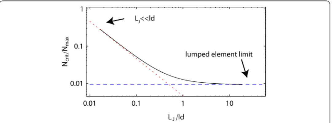
Figure 7 Validity of the quartic approximation.RatioNcrit/Nmaxaccording to Eq.()(black), in the lumped element limit (dashed blue) and in the limit of small participation ratioLJld(dotted red) for the
parameters{ ˜ω0/2π,Q}={7 GHz, 1,000}.
In order to minimize the effect of higher order nonlinearities we want to keep this ratio small. It has the following two interesting limits
Ncrit
Nmax,j
= ⎧ ⎨ ⎩
√
Q –ld
LJ, forLJld,
√
Q
–, for lumped element JPA. ()
This is an important result, which sets clear constraints on both the maximally achievable bandwidth and the dynamic range of the JPA. If we wantNcrit/Nmax,jto be small,κneeds to
be sufficiently small as well. One may also want to increase the dynamic range by reducing the Kerr nonlinearity|K|. While this can in principle be achieved by choosing a small ratio
LJ/ldbetween Josephson and geometric inductance, care has to be taken when using this
approach because additional geometric inductance leads to a larger ratio Ncrit/Nmax as
illustrated in Figure .
Interestingly, we find that in the lumped element case the Josephson inductance LJ,
and with it the Kerr nonlinearityK, can in principle be made smaller without affecting
Ncrit/Nmax. However, in practice a small Josephson inductance has to be compensated
by a large lumped element capacitor to retain the desired resonance frequency, which is challenging to realize without introducing additional parasitic geometric inductances. It therefore seems difficult to build a parametric amplifier with large bandwidth and high dynamic range at the same time using a single SQUID only. In the following we show how
one can keepNcrit/Nmax constant while decreasing the nonlinearity and thus increasing
the dynamic range of the amplifier, by replacing the single SQUID with a serial array ofM
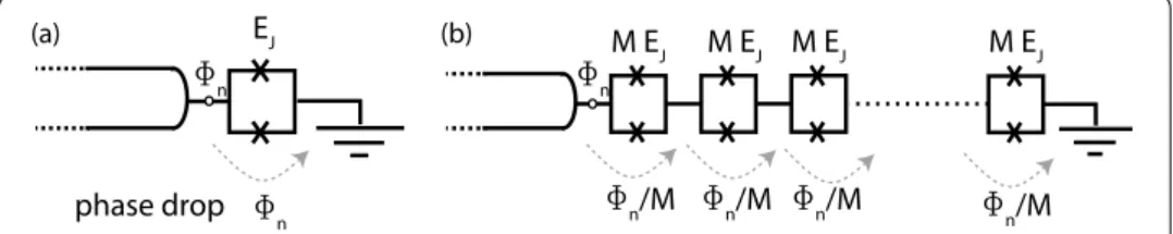
SQUIDs ofM-times larger Josephson energy per SQUID (Figure ).
5.2 Josephson junction arrays
For simplicity we assume that all SQUIDs in the array have the same effective Josephson energyMEJ. Since the spatial extent of the junction is still small compared to typical
reso-nance wavelengths, we can treat the array as a lumped element. To derive the nonlinearity of the oscillator for this situation we investigate how the different terms in the Lagrangian scale withM.
Figure 8 Schematic of the SQUID array.(a) The phase drop across a single SQUID junction is proportional to the node fluxn(indicated by the circle) at the end of the transmission line. (b) If we replace the single
junction by an serial array ofMjunctions withMtimes larger Josephson energy, the phase drop across each junction is by a factor ofMsmaller while the total effective Josephson inductance stays the same.
phase dropn/Macross each SQUID, see Figure . As a result the quadratic term in the
Lagrangian scales as
EJ
n
→M
−→
M
i=
MEJ
n
M
=EJ
n ()
and thus remains constant. This agrees with our expectation, since the total linear Joseph-son inductance has not been changed. However, the quartic term scales like
EJ
n
→M
−→
M
i=
MEJ
n
M
=
M
EJ
n, ()
which leads to a quadratic decrease in the effective Kerr nonlinearityK→K/Mand thus
a quadratic increase inNcrit∝M. Furthermore, the maximal photon number also scales
asNmax∝Msince the critical current of each junction is larger by a factor ofM. In other
words, the ratioNcrit/Nmaxonly depends on the total Josephson inductance whereas the
bifurcation power increases quadratically inM. We thus conclude that the dynamic range
of a JPA can be increased without affecting the amplifier bandwidth, by using an array of SQUIDs instead of a single SQUID. This conclusion is valid for both the transmission line JPA and the lumped element JPA.
In practice, the Josephson energies in the array are not all equal due to inhomogeneous coupling to the external magnetic flux and scatter in the critical current of Josephson junctions due to unavoidable variations in fabrication. A quantitative analysis of the influ-ence of such variations of Josephson energies on the parametric amplifier characteristics could be an interesting task for future studies. This would help to quantify limitations in the accessible tuning range of the parametric amplifier and a realistic understanding of the breakdown of the low order expansion of the cosine potential. For such an approach the methods used in Ref. [] could turn out to be useful.
6 Conclusion
SQUID arrays instead of single SQUIDs provides the possibility to enhance the strength of the pump field close at the bifuraction point and with it the dynamic range of the JPA.
Competing interests
The authors declare they have no competing interests.
Authors’ contributions
All authors contributed equally to the work in this article.
Acknowledgements
The authors would like to acknowledge helpful discussions with Alexandre Blais, Vitaly Shumeiko and Sebastian Schmidt. This work was supported by the European Research Council (ERC) through a Starting Grant and by ETHZ.
Received: 30 May 2013 Accepted: 25 September 2013 Published: 29 January 2014
References
1. Yurke B, Buks E:J Lightwave Technol2006,24:5054.
2. Castellanos-Beltran MA, Lehnert KW:Appl Phys Lett2007,91:083509.
3. Tholén E, Ergül A, Doherty E, Weber F, Grégis F, Haviland D:Appl Phys Lett2007,90:253509. 4. Kinion D, Clarke J:Appl Phys Lett2008,92:172503.
5. Yamamoto T, Inomata K, Watanabe M, Matsuba K, Miyazaki T, Oliver WD, Nakamura Y, Tsai JS:Appl Phys Lett2008,
93:042510.
6. Castellanos-Beltran MA, Irwin KD, Hilton GC, Vale LR, Lehnert KW:Nat Phys2008,4:929. 7. Palacios-Laloy A, Nguyen F, Mallet F, Bertet P, Vion D, Esteve D:J Low Temp Phys2008,151:1034. 8. Kamal A, Marblestone A, Devoret M:Phys Rev B2009,79:184301.
9. Bergeal N, Schackert F, Metcalfe M, Vijay R, Manucharyan VE, Frunzio L, Prober DE, Schoelkopf RJ, Girvin SM, Devoret MH:Nature2010,465:64.
10. Hatridge M, Vijay R, Slichter DH, Clarke J, Siddiqi I:Phys Rev B2011,83:134501. 11. Vijay R, Slichter DH, Siddiqi I:Phys Rev Lett2011,106:110502.
12. Gao J, Vale LR, Mates JAB, Schmidt DR, Hilton GC, Irwin KD, Mallet F, Castellanos-Beltran MA, Lehnert KW, Zmuidzinas J, Leduc HG:Appl Phys Lett2011,98:232508.
13. Eichler C, Bozyigit D, Lang C, Baur M, Steffen L, Fink JM, Filipp S, Wallraff A:Phys Rev Lett2011,107:113601. 14. Abdo B, Kamal A, Devoret M:Phys Rev B2013,87:014508.
15. Kamal A, Clarke J, Devoret MH:Phys Rev B2012,86:144510. 16. Louisell WH, Yariv A, Siegman AE:Phys Rev1961,124:1646. 17. Gordon JP, Louisell WH, Walker LR:Phys Rev1963,129:481. 18. Mollow BR, Glauber RJ:Phys Rev1967,160:1076.
19. Clerk AA, Devoret MH, Girvin SM, Marquardt F, Schoelkopf RJ:Rev Mod Phys2010,82:1155.
20. Mallet F, Castellanos-Beltran MA, Ku HS, Glancy S, Knill E, Irwin KD, Hilton GC, Vale LR, Lehnert KW:Phys Rev Lett2011,
106:220502.
21. Flurin E, Roch N, Mallet F, Devoret MH, Huard B:Phys Rev Lett2012,109:183901.
22. Menzel EP, Di Candia R, Deppe F, Eder P, Zhong L, Ihmig M, Haeberlein M, Baust A, Hoffmann E, Ballester D, Inomata K, Yamamoto T, Nakamura Y, Solano E, Marx A, Gross R:Phys Rev Lett2012,109:250502.
23. Vijay R, Macklin C, Slichter DH, Weber SJ, Murch KW, Naik R, Korotkov AN, Siddiqi I:Nature2012,490:77. 24. Johnson JE, Macklin C, Slichter DH, Vijay R, Weingarten EB, Clarke J, Siddiqi I:Phys Rev Lett2012,109:050506. 25. Ristè D, van Leeuwen JG, Ku H-S, Lehnert KW, DiCarlo L:Phys Rev Lett2012,109:050507.
26. Campagne-Ibarcq P, Flurin E, Roch N, Darson D, Morfin P, Mirrahimi M, Devoret MH, Mallet F, Huard B:Phys Rev X2013,
3:021008.
27. Teufel JD, Donner T, Li D, Harlow JW, Allman MS, Cicak K, Sirois AJ, Whittaker JD, Lehnert KW, Simmonds RW:Nature 2011,475:359.
28. Eichler C, Bozyigit D, Wallraff A:Phys Rev A2012,86:032106.
29. Eichler C, Lang C, Fink JM, Govenius J, Filipp S, Wallraff A:Phys Rev Lett2012,109:240501.
30. Steffen L, Salathe Y, Oppliger M, Kurpiers P, Baur M, Lang C, Eichler C, Puebla-Hellmann G, Fedorov A, Wallraff A:Nature 2013,500:319.
31. Louisell WH:Coupled Mode and Parametric Electronics. New York: John Wiley; 1960. 32. Slusher RE, Hollberg LW, Yurke B, Mertz JC, Valley JF:Phys Rev Lett1985,55:2409. 33. Burnham DC, Weinberg DL:Phys Rev Lett1970,25:84.
34. Bergeal N, Vijay R, Manucharyan VE, Siddiqi I, Schoelkopf RJ, Girvin SM, Devoret MH:Nat Phys2010,6:296. 35. Bergeal N, Schackert F, Frunzio L, Devoret MH:Phys Rev Lett2012,108:123902.
36. Roch N, Flurin E, Nguyen F, Morfin P, Campagne-Ibarcq P, Devoret MH, Huard B:Phys Rev Lett2012,108:147701. 37. Ho Eom B, Day PK, LeDuc HG, Zmuidzinas J:Nat Phys2012,8:623.
38. Yaakobi O, Friedland L, Macklin C, Siddiqi I:Phys Rev B2013,87:144301.
39. Wilson CM, Johansson G, Pourkabirian A, Simoen M, Johansson JR, Duty T, Nori F, Delsing P:Nature2011,479:376. 40. Wustmann W, Shumeiko V:Phys Rev B2013,87:184501.
41. Dykman M, Krivoglaz M:Phys A, Stat Mech Appl1980,104:480. 42. Marthaler M, Dykman MI:Phys Rev A2006,73:042108.
43. Siddiqi I, Vijay R, Pierre F, Wilson CM, Metcalfe M, Rigetti C, Frunzio L, Devoret MH:Phys Rev Lett2004,93:207002. 44. Vijay R, Devoret MH, Siddiqi I:Rev Sci Instrum2009,80:111101.
47. Walls DF, Milburn GJ:Quantum Optics. Berlin: Springer; 1994.
48. Göppl M, Fragner A, Baur M, Bianchetti R, Filipp S, Fink JM, Leek PJ, Puebla G, Steffen L, Wallraff A:J Appl Phys2008,
104:113904.
49. Braunstein SL, van Loock P:Rev Mod Phys2005,77:513. 50. Caves CM:Phys Rev D1982,26:1817.
51. Wallquist M, Shumeiko VS, Wendin G:Phys Rev B2006,74:224506. 52. Bourassa J, Beaudoin F, Gambetta JM, Blais A:Phys Rev A2012,86:013814.
53. Girvin SM:Lectures delivered at Ecole d’Eté Les Houches. To be published by Oxford University Press, 2011. 54. Imoto N, Haus HA, Yamamoto Y:Phys Rev A1985,32:2287.
55. Sanders BC, Milburn GJ:Phys Rev A1989,39:694.
56. Santamore DH, Goan H-S, Milburn GJ, Roukes ML:Phys Rev A2004,70:052105. 57. Buks E, Yurke B:Phys Rev A2006,73:023815.
58. Helmer F, Mariantoni M, Solano E, Marquardt F:Phys Rev A2009,79:052115.
59. Johnson BR, Reed MD, Houck AA, Schuster DI, Bishop LS, Ginossar E, Gambetta JM, DiCarlo L, Frunzio L, Girvin SM, Schoelkopf RJ:Nat Phys2010,6:663.
60. Suchoi O, Abdo B, Segev E, Shtempluck O, Blencowe MP, Buks E:Phys Rev B2010,81:174525.
61. Kirchmair G, Vlastakis B, Leghtas Z, Nigg SE, Paik H, Ginossar E, Mirrahimi M, Frunzio L, Girvin SM, Schoelkopf RJ:Nature 2013,495:205.
62. Koch J, Yu TM, Gambetta J, Houck AA, Schuster DI, Majer J, Blais A, Devoret MH, Girvin SM, Schoelkopf RJ:Phys Rev A 2007,76:042319.
63. Ferguson DG, Houck AA, Koch J:Phys Rev X2013,3:011003.
doi:10.1140/epjqt2