Parametric Modelling of Flexible Plate Structures Using Ant Colony Optimization

AENSI Journals

Australian Journal of Basic and Applied Sciences

ISSN:1991-8178

Journal home page: www.ajbasweb.com

Corresponding Author: N.S.A.A. Jalil, Universiti Kebangsaan Malaysia, Department of Mechanical and Material Engineering, Faculty of Engineering& Built Environment, Malaysia.

E-mail: nsaajalil@siswa. um.edu.my

Parametric Modelling of Flexible Plate Structures Using Ant Colony Optimization

1_{N.S.A.A. Jalil,} 2_{S. Julai,} 1_{R. Ramli}

1_{Universiti Kebangsaan Malaysia, Department of Mechanical and Material Engineering, Faculty of Engineering & Built Environment}

Malaysia.

2_{Universiti Kebangsaan Malaysia , 50300 Kuala Lumpur, Selangor, Malaysia}

A R T I C L E I N F O A B S T R A C T

Article history:

Received 15 April 2014 Received in revised form 22 May 2014

Accepted 25 October 2014 Available online 10 November 2014

Keywords:

Ant colony optimization; parametric identification; flexible plate structures

Background: This paper presents parametric modelling of flexible plate structures using ant colony optimization (ACO). The global optimization technique of ACO is utilized to obtain a dynamic model of a flexible plate structure based on one-step-ahead (OSA) prediction. Objective: The structure is subjected to three different disturbance signal types, namely random, pseudo random binary sequence (PRBS), and finite duration step. The fitness function for the ACO optimization is the mean-squared error (MSE) between the measured and estimated outputs of the plate. Results: The validation of the algorithm is presented in both time and frequency domains. The developed ACO modelling approach will be used for active vibration control systems design and development in future work. Conclusion The performance of ACO2 has been shown to outperform ACO1 in minimizing the prediction error, resulting in a good level of accuracy of the estimated model.

© 2014 AENSI Publisher All rights reserved. To Cite This Article: N.S.A.A. Jalil, S. Julai and R. Ramli., Parametric Modelling of Flexible Plate Structures Using Ant Colony Optimization. Aust. J. Basic & Appl. Sci., 8(19): 258-263 2014

INTRODUCTION

System identification deals with the problem of building mathematical models of dynamical systems based on observed data from the system in either the time or frequency domain. Modeling and identification techniques help develop knowledge about a system. They are prerequisites to many practices in engineering and technology and are especially important in the field of automatic control. Estimation of the parameter values involves uncertainties that are due to limitations of the mathematical models used to represent the behaviour of the real structure, the presence of measurement error in the data, and insufficient excitation and response bandwidth. In model-based control systems design a good model should capture the most important dynamic behaviour of the process in realistic conditions while remaining as simple as possible (Alasty, A., R. Shabani, 2006; Papadimitriou, C., 2004; Sanchez, J.M.M., 1996; Vasquez, J.R.R., 2008).

Ant colony optimization (ACO) is a meta-heuristic inspired by a foraging behaviour of ants that has been effectively applied to tackle hard combinatorial optimization problems. The fundamental component of ACO is a solution structured mechanism, which simulates the decision making processes of ant colonies as they seek for food whereby finally find the most competent route from their nests to food sources. ACO is a probabilistic search approach that is based on inspiration of evolutionary process for the search of resolutions to the various types of optimization problems in continuous domain. The adaptation of the ant colony algorithm to the handling of continuous domain is done by substituting the discrete probability distribution with a continuous one without any major conceptual changes to its construction. Based on the objective values in continuous domain, achieving the global optimal solution can be more abruptly and refined search attempts within expectant regions by self-adjusting the path searching behaviours of the ant. Within the past decade, ACO has attracted and inspired scholar attentions to endeavour improvement and amendment of ACO algorithms.

Flexible Plate Structure:

Flexible structure systems are known to demonstrate an intrinsic property of vibration when subjected to disturbance forces, leading to component and structural damage. Study of the natural modes, frequencies and the dynamic behavior of flexible plates have received considerable attention due to the range of applications, including bridge decks, solar panels, and electronic circuit board design. There is a growing need for developing suitable modeling and control strategies for such systems due to the highly non-linear dynamics of such systems. It is crucial to obtain an accurate model of a plate structure in order to control the vibration of the plate efficiently.

Dynamic modeling and simulation of a flexible plate structure using the finite difference (FD) method have been reported in Darus & Tokhi (2002), where a flat, square plate with all edges clamped has been considered. The classical dynamic equation of a thin rectangular plate is developed using partial differential equation (PDE) derived from Leissa (1969) and Timoshenko & -Krieger (1959).

D q t

w D y

w y x

w x

W _

       

   

2 2 4 4 2 2

4 4 4

2 

(1)

where

w

is the lateral deflection in the

z

direction, r is the mass density per unit area, q = q(x, y) is the transverse external force at point (x, y) and has dimensions of force per unit area,



2

w



t

2 is the acceleration in the z direction,



312(1 )



v Eh

D  is the flexural rigidity with v representing the Poisson ratio, h the thickness of the plate, and E the Young’s modulus. The details of flexible plate equation can be referred to Julai and Tokhi (2010).

Ant Colony Optimization:

The basic ACO algorithm actually fits a discrete problem only and is not suitable for solving continuous optimization problems such as linear or non-linear programming. Applying this algorithm to continuous domains was not straightforward where the main issue is how to model a continuous nest neighbourhood with a discrete structure. As the design problem can always be formulated as optimization problem in continuous design space, the ACO algorithm applied in any field should be modified accordingly (Chen, L., 2003; Socha, K., M. Dorigo, 2008).

The first step in ACO is to initialize all the pheromone. ACO has a common framework which consists of Solution Construction Operator, Pheromone Update Operator and Daemon Action.

Solution construction operator:

The solution construction operator is performed by each ant to construct its routing path (i.e., a solution of the problem) based on the pheromone and heuristic information available. More precisely, the routing path of each ant is constructed edge by edge until the routing path is completely established. The probability of selecting edge eij, i.e., the probability of an ant at subsolution i selecting j as the next subsolution (i.e.,

subsolution i + 1), is defined as

     





 

otherwise , j if

0

] [ ] [

] [ ] [ )

( j

i k

is is

ij ij k

ij t ik

p  

 

 

 

(2)

where Nik denotes the set of candidate subsolutions (i.e., subsolutions that can be selected by ant k at subsolution

i); τij and ηij denote, respectively, the pheromone value and the heuristic value associated with eij.

Pheromone update operator:

The pheromone update will update the pheromone values that are associated with the search experience of ACO. On the other hand, the pheromone evaporation is used to avoid rapid convergence to a local region (Billings, S.A., 1994). The pheromone update operator employed for updating the pheromone value of each edge eij is defined as

ij ij

ij t n



t





(  ) () ₍₃₎

where ρ is a coefficient such that (1 – ρ ) represents the evaporation trail between t and t + n, τij is











m

k k

ij ij

1





(4)

where k

ij













otherwise

j)

(i,

connection

from

goes

ant

k

if

0

th

k ij

L Q k



(5)

where Q is a constant and Lk is the tour length of the kth ant. The coefficient ρ must be set to a value 0 < ρ < 1 to

avoid unlimited accumulation of trail.

Daemon Actions:

This is an optional component which is used to implement centralized actions that cannot be implemented by a single ant, such as local search, and pheromone re-initialization.

ACO1:

The development of ACO1 has been presented in (Quan, H., H. Chao, 2007; Wang, L., Q. Wu, 2001). This algorithm is referred to as ACO1 throughout this work. Here, the optimization problem is solved by a cooperation of artificial ant colony by exchanging information via pheromone deposited on graph edges. The essence of ACO1 is composed of two parts:

1. A state transition rule used by an ant to determine the next destination of a complete tour, and 2. A pheromone updating rule in allocating a greater amount of pheromone to shorten the tour.

Let the vector X = [x1, x2, ..., xn] be the parameters to be optimized, where n represents the total number of

parameters in the AVC system, along with upper and lower bounds to be xi∈D(xi) = [x, xi_up] with i = 1,2, ..., n.

The definition field D(xi) is divided into M subspaces, and the middle of each subspace defines a node.A single

artificial ant k (k = 1, 2, ..., Nant) where Nant is the maximum number of ants, would choose to move from one node to the other, in the total of P nodes ineach D(xi). The length of each sub-space hi can be expressed by

M

x

x

h

i i up i low

_

_





(6)

ACO2:

In ACO2, the eqn (6) is used and m ants are dispatched initially with i = 1,2, ..., n. Based on the amount of pheromone in the regions, the ants choose which region to explore using eqn (7). At first, S grids are created in the search space randomly. Lower (Lo) and upper (Up) bound is set to be [-1,1]. The initialization of the feasible solution by ant is using eqn (8). The procedure is followed by the repetition of the main loop until a termination condition is met, which may be a given number of solution constructions or a limit on the available computation time.

)rand() (Nant

tour  1 ₍₇₎

) ( ) 1 ( )

(i touri hi Lo

tion

initializa     ₍₈₎

Additionally, these solutions may be improved using RWS which stands for the roulette wheel selection. Here the RWS is based on the pheromone value of the regions. A user-defined probability q0 is used to decide whether to select the region with the highest pheromone or the region selected by the RWS method. The probability of the ant choosing region j is given by

  

 _

 

otherwise,

,

, q q if ,

max o

RWS j

j jSRj

(9)

where SR is the set of regions, τj is the pheromone value in region j, q is a uniform random number in [0,1]. The

selected pheromone value using RWS will be used in eqn (10) as follows:

Nant RWS i

Lo i Up i Lo i solution

best_ () ()[ () ()] / ₍₁₀₎

Then, the best solution will be compared with the previous solution and if satisfied, the new best solution found is determined.

Parametric System Identification:

the model. The difference between the outputs from the system and its model, i.e. y(t) and (t) will then be fed into ACO to estimate the unknown parameters for the system model.

After the maximum number of iterations has been reached, the estimated parameters will be used to update the system model, and then the above process will be repeated. Auto-regressive with exogenous (ARX) input structure is chosen to model the system (Ljung, L., T. Glad, 1994). This is expressed as





        n i m j j t u j b i t y i a y 1 0 ^ ) ( ) ( ) ( ) ( (11)

where a(i) , b(j) are denominator and numerator polynomial coefficients, n and m are number of coefficients in the denominator and numerator polynomials, y, u, and yˆ are measured output, input, and estimated output, respectively. The order of the transfer function depends on n. For optimization formula, the mean-squared error (MSE) of the difference between the outputs from the system and its model is used as defined by



       _  s i

error yi yi

S f 1 2 ^ ) ( ) ( 1 min (12)

along with upper and lower bounds on the design variables,



1



a

(

i

)



1

and



1



b

(

i

)



1

as in (10), S represents the number of input/output samples, y(i) is the measured output and yˆ(i) is the calculated model output.

RESULT AND DISCUSSION

An aluminium type plate of dimensions 1.0m×1.0m×0.32mm was divided into 20×20 sections with a sampling time 0.016 sec. The specification of the plate are mass density per area, ρ = 2.71×103 _kg/m2_{, Young’s}

modulus, E = 7.11×1010N/m2, Poisson’s ratio, υ = 0.3, moment of inertia, Ι = 5.1924×10-11kg.m2 and simulation time, t = 4 seconds. Tests were carried out with different disturbance signal types, namely random, pseudo random binary sequence (PRBS) and finite duration step. The disturbance source, detection point, and observation point were arranged at locations (7, 7), (8, 8) and (9, 14). Here the system is characterized with the detected signal as input and observed signal as output. The best result for ACO2 obtained with 15 ants in 600 iterations.

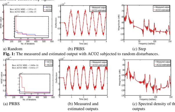
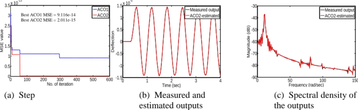
Figure 1, 2 and 3 show results of the measured and estimated output obtained with ACO2 algorithm subjected to different disturbance signal types. ACO1 was also realized for reasons of comparison of modeling in the system. As shown in figures 2(a), 3(a) and 4 (a), the ACO2 achieved the best MSE levels of 1.148×10-15, 6.641×10-17, 1.148×10-15 in the 283rd , 521st and 57th iterations, respectively, for modelling using random, PRBS and finite duration step signals.

a) Random (b) PRBS (c) Step

Fig. 1: The measured and estimated output with ACO2 subjected to random disturbances.

(a) PRBS (b) Measured and estimated outputs

(c) Spectral density of the outputs

Fig. 2: The measured and estimated output with ACO2 subjected to PRBS disturbances.

0 100 200 300 400 500 600 0

1 2 3 4 5x 10

-13

No. of iterations

M S E va lu e ACO1 ACO2

Best ACO1 MSE = 1.951e-15 Best ACO2 MSE = 1.148e-15

0 1 2 3 4

-1.5 -1 -0.5 0 0.5 1 1.5x 10

-6 Time (sec) De fle ct io n Measured output ACO2-estimated

0 1 2 3 4

-3 -2 -1 0 1 2 3x 10

-7 Time (sec) De fle ct io n Measured output ACO2-estimated

0 50 100 150

-120 -110 -100 -90 -80 -70 -60 Frequency (rad/sec) M a g n itu d e ( d B ) Measured output ACO2-estimated

0 50 100 150

-140 -130 -120 -110 -100 -90 -80 -70 Frequency (rad/sec) M a g n itu d e ( d B ) Measured output ACO2-estimated

0 100 200 300 400 500 600 0 0.2 0.4 0.6 0.8 1 1.2 1.4x 10

-14

No. of iterations

M S E va lu e ACO1 ACO2

Best ACO1 MSE = 1.869e-16 Best ACO2 MSE = 6.641e-17

20 40 60 80 0.5 1 1.5 2 2.5 3 x 10-15

20 40 60 80 0 1 2 3 4 5 6 7

(a) Step (b) Measured and estimated outputs

(c) Spectral density of the outputs

Fig. 3: The measured and estimated output with ACO2 subjected to finite duration step disturbances.

Computational time is one of the important factors to be considered in an optimization process. For comparison, at the average time of 120 sec, ACO1 achieved the best MSE levels of 1.951×10-15, 1.869×10-16, 9.116×10-14 in the 167th , 467th and 297th iterations, respectively, for modelling using random, PRBS and finite duration step signals. On the other hand, at the same iteration with ACO1, the value of MSE obtained by ACO2 is 1.9732×10-15, 7.5640×10-17 respectively for random and PRBS signals. Thus, the performance of ACO2 has improved with the use of RWS in the modeling of the flexible plate.

Conclusions:

In this work, the system identification problem has been formulated as an optimization task where ACO2 has been used to estimate parameters of the flexible plate model so as to minimize the prediction error between the measured and estimated outputs at each time step. The vibration modes of the flexible plate structure have been detected successfully with the modelling techniques considered in this investigation. OSA prediction model has been used to identify the parameters with model validity tests using correlation tests. ACO2 has been shown to outperform ACO1 in minimizing the prediction error, resulting in a good level of accuracy of the estimated model.

ACKNOWLEDGEMENT

Authors would like to express their gratitude to Minister of Higher Education of Malaysia, University Malaya (Research University Grant No. RG 117 11AET) for funding and providing facilities to conduct the research.

REFERENCES

Alasty, A., R. Shabani, 2006. Nonlinear parametric identification of magnetic bearings. Mechanics, 16(8): 451-459.

Billings, S.A., Q.M. Zhu, 1994. Nonlinear model validation using correlation tests. International Journal of Control, 60(6): 1107-1120.

Chen, L., J. Shen, L. Qin, H.J. Chen, 2003. An improved ant colony algorithm in continuous optimization. Systems Science and Systems Engineering, 12(2): 224-235.

Darus, I.Z.M., M.O. Tokhi, 2002. Modelling of flexible plate structure using finite difference method. Paper

presented at the 2nd World Engineering Conferenc, Malaysia.

Julai, S., M.O. Tokhi, 2010. Vibration suppression of flexible plate structures using swarm and genetic optimization techniques. Journal of Low Frequency Noise, Vibration and Active Control, 29(4).

Leissa, A.W., 1969. VIbration of Plates. Washington D. C.: NASA SP-60.

Ljung, L., T. Glad, 1994. Modelling of Dynamic Systems. New Jersey: Prentice-Hall.

Papadimitriou, C., 2004. Optimal sensor placement methodology for parametric identification of structural systems. Journal of Sound and Vibration, 278: 923-947.

Quan, H., H. Chao, 2007. Satellite constellation design with adaptively continuous ant system algorithm. Chinese Journal of Aeronautics, 20(4): 297-303.

Sanchez, J.M.M., 1996. Adaptive predictive control: From the concepts to plan optimization. New Jersey: Prentice-Hall.

Socha, K., M. Dorigo, 2008. Ant colony optimization for continuous domains. European Journal of Operational Research, 185(3): 1155-1173. doi: 10.1016/j.ejor.2006.06.046.

Timoshenko, S., S.W. Krieger, 1959. Theory of plates and shells. New York: McGraw-Hill Book Company.

Vasquez, J.R.R., R.R. Perez, J.S. Moriano, J.R.P. Gonzalez, 2008. System identification of steam pressure in a fire-tube boiler. Computers & Chemical Engineering, 32(12): 2839-2848.

0 50 100 150 -90

-80 -70 -60 -50 -40 -30

Frequency (rad/sec)

M

a

g

n

itu

d

e

(

d

B

)

Measured output ACO2-estimated

0 1 2 3 4

-1.5 -1 -0.5 0 0.5 1 1.5x 10

-5

Time (sec)

De

fle

ct

io

n

Measured output ACO2-estimated

0 100 200 300 400 500 600 0

0.5 1 1.5 2 2.5 3 3.5x 10

-13

No. of iteration

M

S

E

va

lu

e

ACO1 ACO2