ISSN:1991-8178
Australian Journal of Basic and Applied Sciences
Journal home page: www.ajbasweb.com
Corresponding Author: Sahil Garg, Universiti Teknologi Petronas, Department of Chemical Engineering, 32610 Bandar Seri Iskandar, Perak Darul Ridzuan, Malaysia.
Tel: +60 165307338; E-mail: [email protected]
A Neural Network Approach to Predict the Density of Aqueous MEA Solution
Sahil Garg, Azmi Mohd Shariff, M.S. Shaikh, Bhajan Lal, Asma Aftab and Nor Faiqa
Universiti Teknologi Petronas, Department of Chemical Engineering, 32610 Bandar Seri Iskandar, Perak Darul Ridzuan, Malaysia.
A R T I C L E I N F O A B S T R A C T Article history:
Received 10 October 2015 Accepted 30 November 2015 Available online 31 December 2015
Keywords:
Density; Aqueous MEA; CO2 capture;
Neural Networks
Background: Aqueous solution of alkanolamines such as MEA, DEA and MDEA has
been used as the potential solvents for the removal of acidic gases like CO2 and H2S
from power plants and various other industries. Objective: A computational model based on artificial neural networks (ANNs) has been developed to predict the density of aqueous MEA solution. Statistical analysis of the predicted data has also been performed. Results: A good agreement was found between the predicted and literature data. Conclusion: The value of low predicted error via statistical analysis showed that the applied model can successfully predict the density of the aqueous MEA solution.
© 2015 AENSI Publisher All rights reserved. To Cite This Article: Sahil Garg, Azmi Mohd Shariff, M.S. Shaikh, Bhajan Lal, Asma Aftab and Nor Faiqa., A Neural Network Approach
to Predict the Density of Aqueous MEA Solution. Aust. J. Basic & Appl. Sci., 9(37): 415-422, 2015
INTRODUCTION
Lately, it has been shown that global warming is one of the main environmental issues due to the increasing concentration of carbon dioxide (CO2)
(Mondal et al., 2015). It is subsequently important to develop and utilize efficient techniques for CO2 gas
removal. Post-combustion capture using absorption is one of the most widely used technique to remove CO2 and alkanolamines have long been recognized as
viable solvents for CO2 removal in industries and
power plants. Due to the strong base nature and fast reactivity with CO2, aqueous monoethanolamine
(MEA) is still considered as the most popular solvents for CO2 capture in industries (Wong et al.,
2015).
Physiochemical properties such as density of aqueous MEA is very important for the analysis of absorption and desorption processes (Shaikh et al., 2014; Teng et al., 1994). Many studies have been done to find out the density of aqueous MEA at different concentration and temperature conditions. But the measurement of density of aqueous MEA at different other temperatures and concentrations is very costly, time-consuming and difficult. So, lately, a new computational prediction technique named artificial neural network (ANN) has attracted great attention. For example, Golzar et al. (2014) has used multilayer perceptron ANN model to predict the thermophysical properties of binary mixtures of common ionic liquids with water or alcohol.
In this study, a computational model based on ANNs was developed to predict the density of
aqueous MEA solution. All the data used in this work was taken from literature (Han et al., 2012). A statistical analysis of the data was performed in terms of least square correlation (R2), root mean square error (RMSE), average relative deviate (ARD), standard deviation (SD) and average absolute deviation (AAD).
MATERIALS AND METHODS
The following subsections provide information about the density database utilized, ANN, and the model used, as well as the parameters and optimization processes.
Density database of aqueous MEA solution: The data used in this work for the prediction of density of aqueous MEA solution was taken from Han et al., (2012). A total of 180 data sets were taken and used to develop a computational model.
Artificial Neural Network Model:
Each neuron is associated with a set of some input connections as the processing elements and as
well as the single output, shown in Fig. 1.
Fig. 1: Schematic of components of simple neuron.
The expression for output activation can be described as follows:
( )
x =g( )
a( )
x =g(
b+∑
iwixi)
h
The function g(a(x)) is denoted as the activation function, where b is the neuron bias present in the neural network, it is biased because in case of no inputs then b would be the pre-activation.
w is the connection weight vector, described as:
[
w w w wN]
w= 1, 2, 3,....,
And x is the input vector, described as:
[
x x x xN]
x= 1, 2, 3,....,
The specific model proposed in this work for the prediction of density data is multilayer perceptron (MLP), the most common type of ANN (Torrecilla et
al., 2007).
Multilayer perceptron model (MLP):
A multilayer perceptron (MLP) is feed-forward neural network which needs a preferred output in order to learn. A MLP neural network comprises of input layer, hidden layer and output layer. The point of MLP neural network is to make a model that appropriately maps a set of input information onto a set of suitable outputs utilizing historic information so that the model can be used to generate an output when the preferred output is vague (Nikravesh and Aminzadeh, 2001). In order to train the network, MLP utilizes a supervising learning technique known as back-propagation. In this technique, at first, all the weights are adjusted arbitrarily, then the output is compared with the targeted values in the training sets and the desired error is propagated back into the network. This procedure is repeated continuously until the outputs are acceptably close to the target values (Celikoglu, 2006; Wu and Liu, 2012).
Training neural networks:
When a neural network is formed for a specific application, it is prepared to be trained. Training is the methodology by which connection weights are assumed. Initially, the weights are picked up haphazardly. There are two types of training methodology: supervised and un-supervised training. Supervised training (ST) is refined by providing neural network a set of sample data alongside the expected output from each of these samples. ST is
the most widely recognized type of neural network training. As the ST starts, the neural network is taken through a series of iterations or epochs till the time the output data matches with the targeted data with a sensibly small error. Unsupervised training (UST) is similar to ST with the exception that no targeted values are provided. UST generally arises when neural network characterize the inputs into some groups (Mirarab et al., 2014).
Validating neural networks:
After the neural network is trained, it must be assessed to check whether it is prepared for genuine use. This step is vital to be deliberately performed to figure out whether additional training is needed. To accurately validate a neural network, different data sets for validation must be kept aside from training data sets. It is exceptionally essential that different data sets may be for validation. Training the neural network with a desired set and furthermore utilizing the same set to predict the error of the whole neural network will most likely prompt to bad results. The error obtained utilizing the training sets will considerably be lower than the error on the remaining data sets of neural network. The reliability of the validated data must be maintained continuously. In the event that validation is performed poorly, this probably implies that there was data present in the validation set that was not accessible in the training set. The way that this condition should be resolved is by attempting an alternate, more arbitrary, method for differentiating the data into training and validation sets. If it fails, the validation and training sets must be merged together as one huge training set. At that point, new data must be obtained to serve as the validation data. In some situations, it may be difficult to acquire additional data for either training or validation. While this methodology will do without the security of a proper validation, if additional data cannot be acquired, this may be the only alternative (Mirarab et
al., 2014).
Testing neural networks:
helpful to plot the test error during the training process. In the event that the error in the test set reaches a minimum value at a different iteration number than the validation set error, this may show that the data sets are poorly divided. The existence of irregular noise can also have a significant impact on the capability of neural network to separate between cases near decision limits which will lead to inaccurate predictions (Mirarab et al., 2014).
Optimization procedure:
The optimal design of the artificial neural network (ANN) was figured out by trial and error
method. In this study, the number of neurons in the hidden layers was found out by optimizing the mean-squared error (MSE). Actually, a low number of neurons may not result in enabling a network to achieve the anticipated error, while a large number may cause over fitting. The performance of ANN was assessed by calculating the MSE versus number of neurons, as shown in Fig. 2. It is apparent from Fig. 2 that the lowest MSE was obtained with nine neurons. Therefore, nine neurons were selected as the optimum condition for the present study.
Fig. 2: Variation of Performance (MSE) with number of neurons.
RESULTS AND DISCUSSION
Prediction of density using ANNs:
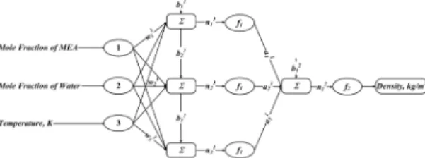
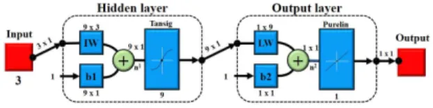
In this study, a total of 180 data points were utilized from literature to analyze the prediction performance of ANN technique. Mole fraction of water, mole fraction of MEA and operational temperature was taken as input variables, while density was assigned as output. All the 180 data points were randomly divided into three data sets, i.e. 70% for training (126 data points), 15% for validation (27 data points) and 15% for testing (27 data points).
For density prediction of aqueous MEA, a multilayer perceptron (MLP) model of ANN was utilized with back propagation algorithm. This specific model was chosen based on their capability to represent the non-linear relationship between input and output data. Levenberg-Marquardt was utilized as a training function for MLP neural network due to its good performance in non-linear regression problems (Mirarab et al., 2014). The optimum number of neurons in hidden layer was chosen by optimization procedure. Tan-sigmoid transfer function was used to train the MLP neural-network (Fig. 3). Therefore, in our study, nine neurons were selected in the hidden layers.
Fig. 3: Artificial Neural Network (ANN) design for prediction of density.
The performance analysis of prediction data for training, validation and testing data-sets was done in terms of mean square error (MSE). So, a graph of MSE vs epochs was plotted for training, validation and testing data-sets to get the best neural network configuration as shown in Fig. 4. It is clearly seen from Fig. 4 that the MSE values decreased as the
number of epochs increased because the weights have been updated after each epoch.
agreement with the literature data. Table 1 summarizes the literature and predicted data of
aqueous MEA with corresponding data sets used in the ANN modeling.
Fig. 4: Variation of Performance (MSE) vs Epochs for training, validation and testing data sets.
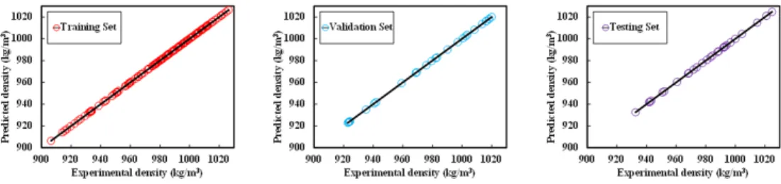
Fig. 5: Evaluation of ANN predicted and experimental data of density for training, validation and testing data sets.
Validation performed in the developed model is done by means of external test based on the following statistical quantities:
Least-squared correlation (R2):
( )
∑
∑
∑
= = − = = = = − − − − − = n i i i n i i i i n i i i x x y x x x R 1 2 1 2 1 2 2Root mean square error (RMSE):
( ) n x y RMSE n i i i i
∑
= = − = 1 2Average relative deviation (ARD):
n x y x ARD n i i i i i
∑
= = − = 1Standard deviation (SD):
∑
= − − − − = ini i x x n SD 1 2 1 1
Average absolute deviation (AAD):
n y x AAD n i i i i
∑
= = − = 1Table 1: Experimental and predicted data of density with corresponding data sets used in ANN modeling.
Run No. Temperature (K) Mole Fraction Density (kg/m3
)
x[MEA] x[H2O] Experimental Predicted
Training Set
1 298.15 0 1 997 996.99270
2 298.15 0.1122 0.8878 1010.9 1010.83227
3 298.15 0.2278 0.7722 1021.3 1021.16469
4 298.15 0.4077 0.5923 1026.3 1026.29901
5 298.15 0.5412 0.4588 1024.7 1024.72866
6 298.15 1 0 1011.9 1011.85753
7 303.15 0 1 995.6 995.60765
8 303.15 0.1122 0.8878 1008.4 1008.59162
9 303.15 0.1643 0.8357 1013.8 1013.69935
10 303.15 0.3067 0.6933 1021.4 1021.45642
11 303.15 0.4077 0.5923 1022.8 1022.82980
12 303.15 1 0 1008 1007.98017
13 308.15 0.1122 0.8878 1006.2 1006.20062
14 308.15 0.1643 0.8357 1011 1011.01756
15 308.15 0.2278 0.7722 1015.2 1015.25074
16 308.15 0.4077 0.5923 1019.3 1019.26992
17 308.15 0.5412 0.4588 1017.3 1017.33607
18 308.15 0.7264 0.2736 1012.3 1012.37012
19 308.15 1 0 1004 1004.04496
21 313.15 0.2278 0.7722 1012.1 1012.14469
22 313.15 0.4077 0.5923 1015.7 1015.65006
23 313.15 0.7264 0.2736 1008.5 1008.45972
24 318.15 0.1122 0.8878 1001.1 1001.02991
25 318.15 0.1643 0.8357 1005.3 1005.32451
26 318.15 0.2278 0.7722 1009 1008.95781
27 318.15 0.3067 0.6933 1011.4 1011.34403
28 318.15 0.4077 0.5923 1012 1011.99048
29 318.15 0.5412 0.4588 1009.7 1009.71062
30 318.15 1 0 996 996.02352
31 323.15 0 1 988 988.00682
32 323.15 0.1122 0.8878 998.1 998.26626
33 323.15 0.2278 0.7722 1005.6 1005.69385
34 323.15 0.3067 0.6933 1007.8 1007.85711
35 323.15 0.4077 0.5923 1008.3 1008.29865
36 323.15 0.5412 0.4588 1005.9 1005.86738
37 328.15 0 1 985.7 985.65316
38 328.15 0.1122 0.8878 995.5 995.39171
39 328.15 0.1643 0.8357 999.2 999.23367
40 328.15 0.2278 0.7722 1002.4 1002.35352
41 328.15 0.3067 0.6933 1004.4 1004.31514
42 328.15 0.4077 0.5923 1004.6 1004.57272
43 328.15 0.5412 0.4588 1002 1002.01007
44 333.15 0.1643 0.8357 996.1 996.04696
45 333.15 0.2278 0.7722 999 998.93687
46 333.15 0.3067 0.6933 1000.7 1000.71468
47 333.15 0.4077 0.5923 1000.8 1000.80631
48 333.15 0.5412 0.4588 998.2 998.13104
49 333.15 0.7264 0.2736 992.7 992.62845
50 333.15 1 0 983.9 983.83242
51 338.15 0 1 980.5 980.49582
52 338.15 0.1122 0.8878 989.5 989.33373
53 338.15 0.2278 0.7722 995.4 995.44392
54 338.15 0.4077 0.5923 997 996.99162
55 338.15 0.5412 0.4588 994.2 994.21871
56 338.15 1 0 979.8 979.77774
57 343.15 0.1122 0.8878 986.1 986.16073
58 343.15 0.1643 0.8357 989.4 989.40504
59 343.15 0.2278 0.7722 991.9 991.87467
60 343.15 0.3067 0.6933 993.2 993.32364
61 343.15 0.4077 0.5923 993.1 993.12119
62 343.15 0.5412 0.4588 990.2 990.26102
63 343.15 0.7264 0.2736 984.6 984.64266
64 348.15 0 1 974.8 974.81668
65 348.15 0.1643 0.8357 985.9 985.95350
66 348.15 0.2278 0.7722 988.3 988.22877
67 348.15 0.3067 0.6933 989.5 989.52662
68 348.15 0.4077 0.5923 989.2 989.18869
69 348.15 0.5412 0.4588 986.2 986.24754
70 348.15 0.7264 0.2736 980.6 980.59060
71 348.15 1 0 971.6 971.64969
72 353.15 0.1643 0.8357 982.4 982.41521
73 353.15 0.3067 0.6933 985.6 985.65857
74 353.15 0.4077 0.5923 985.2 985.18966
75 353.15 0.7264 0.2736 976.5 976.48317
76 353.15 1 0 967.5 967.54891
77 358.15 0.1122 0.8878 976.1 976.09108
78 358.15 0.1643 0.8357 978.7 978.78866
79 358.15 0.3067 0.6933 981.8 981.71790
80 358.15 0.4077 0.5923 981.2 981.12180
81 358.15 0.5412 0.4588 978 978.02690
82 358.15 0.7264 0.2736 972.3 972.31411
83 358.15 1 0 963.4 963.40991
84 363.15 0 1 965.3 965.41159
85 363.15 0.1122 0.8878 972.5 972.54587
86 363.15 0.1643 0.8357 975 975.07149
87 363.15 0.2278 0.7722 976.9 976.82083
88 363.15 0.3067 0.6933 977.7 977.70396
89 363.15 0.4077 0.5923 977.1 976.98525
90 363.15 1 0 959.2 959.22865
91 373.15 0 1 958.6 958.53860
92 373.15 0.1122 0.8878 965.3 965.15308
93 373.15 0.1643 0.8357 967.2 967.35688
94 373.15 0.2278 0.7722 969 968.81277
95 373.15 0.5412 0.4588 965.3 965.21466
96 373.15 0.7264 0.2736 959.3 959.45391
97 373.15 1 0 950.9 950.74753
98 383.15 0 1 951.2 951.16862
99 383.15 0.1122 0.8878 957.4 957.34783
100 383.15 0.3067 0.6933 960.8 960.94596
101 383.15 0.4077 0.5923 959.8 959.82462
102 383.15 0.5412 0.4588 956.5 956.42573
103 383.15 0.7264 0.2736 950.6 950.67065
104 393.15 0 1 943.4 943.32275
105 393.15 0.1122 0.8878 949.1 949.14641
106 393.15 0.3067 0.6933 952.1 952.19584
107 393.15 0.4077 0.5923 950.9 950.94956
108 393.15 0.5412 0.4588 947.6 947.50731
109 393.15 1 0 933.5 933.48524
110 403.15 0.1643 0.8357 941.9 942.06811
111 403.15 0.2278 0.7722 943.1 942.99736
112 403.15 0.5412 0.4588 938.6 938.45977
113 403.15 0.7264 0.2736 932.7 932.84226
115 413.15 0 1 926.3 926.33830
116 413.15 0.1122 0.8878 931.7 931.62617
117 413.15 0.1643 0.8357 932.9 932.96594
118 413.15 0.2278 0.7722 934 933.81835
119 413.15 0.3067 0.6933 933.8 933.97909
120 413.15 0.5412 0.4588 929.3 929.18718
121 413.15 1 0 915.7 915.69527
122 423.15 0 1 917.1 917.15144
123 423.15 0.1122 0.8878 922.3 922.21163
124 423.15 0.5412 0.4588 919.5 919.54473
125 423.15 0.7264 0.2736 914.1 914.13966
126 423.15 1 0 906.4 906.37070
Validation set
127 298.15 0.1643 0.8357 1016.3 1016.24908
128 298.15 0.7264 0.2736 1020 1019.97633
129 303.15 0.2278 0.7722 1018.2 1018.26485
130 303.15 0.7264 0.2736 1016.2 1016.21613
131 308.15 0.3067 0.6933 1018.2 1018.15288
132 313.15 0.1122 0.8878 1003.5 1003.67682
133 313.15 0.1643 0.8357 1008.3 1008.22279
134 313.15 0.5412 0.4588 1013.5 1013.53844
135 318.15 0 1 990.2 990.19181
136 323.15 0.1643 0.8357 1002.3 1002.32716
137 323.15 0.7264 0.2736 1000.6 1000.55254
138 338.15 0.3067 0.6933 997.1 997.05200
139 343.15 1 0 975.8 975.72152
140 348.15 0.1122 0.8878 983 982.89602
141 353.15 0.1122 0.8878 979.4 979.54005
142 353.15 0.5412 0.4588 982.1 982.17075
143 358.15 0 1 968.6 968.66456
144 373.15 0.3067 0.6933 969.4 969.45973
145 383.15 0.1643 0.8357 959.1 959.26831
146 403.15 0 1 935.1 935.04195
147 403.15 0.1122 0.8878 940.6 940.57638
148 403.15 0.4077 0.5923 941.9 941.89977
149 413.15 0.7264 0.2736 923.6 923.66691
150 423.15 0.1643 0.8357 923.3 923.43058
151 423.15 0.2278 0.7722 924.3 924.23176
152 423.15 0.3067 0.6933 924.1 924.33899
153 423.15 0.4077 0.5923 922.8 922.92461
Testing set
154 298.15 0.3067 0.6933 1024.8 1024.66160
155 303.15 0.5412 0.4588 1021 1021.07644
156 308.15 0 1 994 994.00377
157 313.15 0.3067 0.6933 1014.7 1014.77733
158 313.15 1 0 1000 1000.05633
159 318.15 0.7264 0.2736 1004.5 1004.51245
160 323.15 1 0 992 991.96308
161 328.15 0.7264 0.2736 996.7 996.59193
162 328.15 1 0 988 987.89476
163 333.15 0 1 983.2 983.14499
164 333.15 0.1122 0.8878 992.3 992.41228
165 338.15 0.1643 0.8357 992.7 992.76996
166 338.15 0.7264 0.2736 988.7 988.65045
167 343.15 0 1 977.7 977.71704
168 353.15 0 1 971.8 971.79896
169 353.15 0.2278 0.7722 984.5 984.50538
170 358.15 0.2278 0.7722 980.8 980.70320
171 363.15 0.5412 0.4588 973.9 973.81634
172 363.15 0.7264 0.2736 968.1 968.08259
173 373.15 0.4077 0.5923 968.5 968.51752
174 383.15 0.2278 0.7722 960.6 960.48864
175 383.15 1 0 942.3 942.15172
176 393.15 0.1643 0.8357 950.7 950.82941
177 393.15 0.2278 0.7722 952 951.87621
178 393.15 0.7264 0.2736 941.7 941.80301
179 403.15 0.3067 0.6933 943.1 943.22401
180 413.15 0.4077 0.5923 932.6 932.60333
Where xi, yi,x,y andnthe experimental data, predicted data, mean experimental data, mean predicted data and the number of data points respectively. The acquired results of above mentioned statistical quantities (R2, RMSE, ARD, SD and AAD) for density of the predicted model focused around ANN for every three sets (training, validation and testing) as well as the total data set was arranged in Table 2. From table 2, it can be presumed that the three chosen input parameter (temperature, mole fraction of MEA and water) were suitable for predicting the density and the predicted results by the model are dependable on the grounds that their correlation and error values were in a satisfactory range. Furthermore, R2 values of the predicted model
were very near to unity and their relating errors are very small (or negligible).
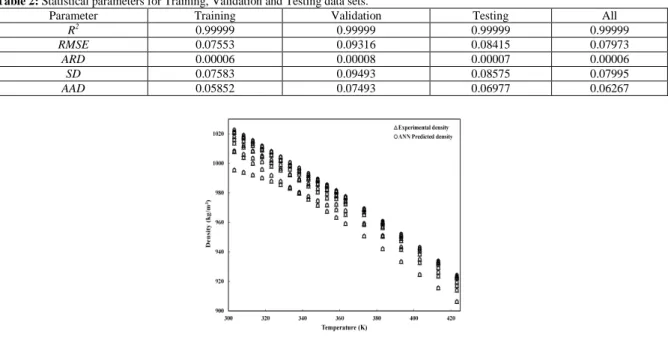
The plot of density data versus operational temperature for the literature data and ANN predicted data is shown in Fig. 6. It can been seen that predicted data showed excellent harmony with the literature data, demonstrating the applicability of ANN model to predict the density of aqueous MEA.
Table 2: Statistical parameters for Training, Validation and Testing data sets.
Parameter Training Validation Testing All
R2 0.99999 0.99999 0.99999 0.99999
RMSE 0.07553 0.09316 0.08415 0.07973
ARD 0.00006 0.00008 0.00007 0.00006
SD 0.07583 0.09493 0.08575 0.07995
AAD 0.05852 0.07493 0.06977 0.06267
Fig. 6: Density as a function of temperature for experimental data and ANN predicted data.
Fig. 7: Comparison of Experimental data with ANN predicted data in different data sets.
Conclusion:
In the present work, we have developed a model using the nonlinear artificial neural network (ANN) technique to predict the experimental density data of aqueous MEA based on temperature and mole fraction of MEA and water. The predicted results disclose that the chosen parameters i.e. inputs, were extremely suitable for the estimation of density of aqueous MEA. In addition, the statistical quality represented by different parameters and the low anticipated error of the developed model show that it can precisely anticipate the density of the aqueous MEA solution.
REFERENCES
Celikoglu, H.B., 2006. Application of radial basis function and generalized regression neural networks in non-linear utility function specification for travel mode choice modelling. Mathematical and Computer Modelling, 44: 640-658.
Golzar, K., S. Amjad-Iranagh, H. Modarress, 2014. Prediction of Thermophysical Properties for Binary Mixtures of Common Ionic Liquids with
Water or Alcohol at Several Temperatures and Atmospheric Pressure by Means of Artificial Neural Network. Ind. Eng. Chem. Res., 53: 7247-7262.
Han, J., J. Jin, D.A. Eimer, M.C. Melaaen, 2012. Density of Water (1) + Monoethanolamine (2) + CO2
(3) from (298.15 to 413.15) K and Surface Tension of Water (1) + Monoethanolamine (2) from (303.15 to 333.15) K. J. Chem. Eng. Data, 57: 1095-1103.
Mirarab, M., M. Sharifi, B. Behzadi, M.A. Ghayyem, 2014. Intelligent Prediction of CO2 Capture in Propyl Amine Methyl Imidazole Alanine Ionic Liquid: An Artificial Neural Network Model. Separation Science and Technology, 50: 26-37.
Nikravesh, M., F. Aminzadeh, 2001. Mining and fusion of petroleum data with fuzzy logic and neural network agents. Journal of Petroleum Science and Engineering, 29: 221-238.
Shaikh, M.S., A.M. Shariff, M.A. Bustam, G. Murshid, 2014. Physicochemical Properties of Aqueous Solutions of Sodium l-Prolinate as an Absorbent for CO2 Removal. J. Chem. Eng. Data, 59:
Teng, T.T., Y. Maham, L.G. Hepler, A.E. Mather, 1994. Measurement and prediction of the density of aqueous ternary mixtures of methyldiethanolamine and diethanolamine at temperatures from 25°c to 80°c. The Canadian Journal of Chemical Engineering 72, 125-129.
Torrecilla, J.S., M.L. Mena, P. Yáñez-Sedeño, J. García, 2007. Application of artificial neural network to the determination of phenolic compounds in olive oil mill wastewater. Journal of Food Engineering, 81: 544-552.
Wong, M.K., M.A. Bustam, A.M. Shariff, 2015. Chemical speciation of CO2 absorption in aqueous
monoethanolamine investigated by in situ Raman spectroscopy. Int. J. Greenhouse Gas Control, 39: 139-147.
Wu, J.D., J.C. Liu, 2012. A forecasting system for car fuel consumption using a radial basis function neural network. Expert Systems with Applications, 39: 1883-1888.