One-layer Neural Network for Solving Least Absolute Deviation Problems with Box
and Equality Constraints
ABSTRACT: In this paper, I design a new neural network for solving least absolute deviation problems with equality and box constraints. Compared with some existing models, the proposed neural network needs the fewest state variables and has only one-layer structure. By constructed a proper Lyapunov function, the following two results can be proved. First, it is stable in the sense of Lyapunov. Second, the solution of the proposed model can converge to an exact optimal solution of the problem. Finally, its validity and transient behaviors are demonstrated by some simulation results.
Keywords: Least Absolute Deviation, Neural Network, One-layer, Lyapunov Stable
Received: 3 December 2017, Revised 27 January 2018, Accepted 7 February 2018
DOI: 10.6025/jes/2018/8/2/57-71
© 2018 DLINE. All Rights Reserved
1. Introduction
Consider the following least absolute deviation problem:
where x = (x1, x2,..., xn)T∈Rn is the decision vector, A ∈ Rm x n, C ∈ Rp x n, b∈Rm, d ∈Rp, rank (C) = p < n are given parameters.
X = {x∈Rn| l < x < h} is a nonempty box set, where l, h ∈Rn (l < h) and some components of l or h can be -∞ or ∞, suitably.
As we know, (1) is called a least absolute deviation problem (see [5-7, 9, 10, 12, 27]), which often encountered in signal processing as an l1-norm optimization problem.
Cuiping Li
Shaanxi Normal University China
(1) min || Ax−b|| 1
In there, x denotes the vector to be estimated, A stands for the model matrix, b is the vector of observation, the noise and errors contained in b is dened as ||Ax − b||1, where ||.||1 denotes l1-norm in this paper. Cx = d and x∈X are constraints where we try to estimate x, conforming to min ||Ax − b||1.
Due to their excellent properties, especially the sparsity properties of the solution, least absolute deviation problems have been extensively studied by many scholars in the past decades. In the early stage, many numerical analysis methods were proposed for solving them have achieved good results (see [14-16]), while they maybe nor satisfy the requirement of real-time. Because the times they consumed in computing a solution is mainly dependent on the dimension and architecture of the problem, and the complexity of the algorithm they applied. Thus, in recent twenty years, a large number of neural network models which can be implemented by VLSI in parallel and competent for real time applications [32], have been designed and can be used to least absolute deviation problems (see [5-13, 19, 27, 30-32]) after [17] and [18]. Since least absolute deviation problems can be rewritten as minimax problems, models in [21- 23, 25, 26, 28, 29, 33] can also be applied to these problems.
For the models presented in the above references, the neural network in [31] can be used to solve (1) and requires only n + p state variables, but it is discontinuous. The models in [9, 30, 32] were designed to solve the min || x||1 problem, the first two include equality constraints and the third has equality and box constraints. They are two special cases of (1), thus cannot be used to (1) if A ≠ In, b ≠ 0 or X is not empty, where Inis a identity matrix of order n in this paper. The models proposed by Xia at. al. and Wang
at. al. in [5, 6, 8] can solve (1) without any constraints, thus they cannot be used to solve (1) when C ≠ 0 or X is not empty. After that, [22], [23] and [10] present three models can be solve (1) with only box constraints. Even though these models have good stability performances, they are hard to solve (1) unless C is invertible. Furthermore, if C is invertible, there will be only one solution for (1) which can be resulted from Cx = d and adjusted by X. The model in [7] can be applied to (1), while it requires m + 3n + 2p state variables and has two-layer structure (see (13) in Section 2). Furthermore, its solution may be feasible but not optimal in some case. (see [27, 32] and Example 1 in Section 3). The model proposed by Xue and Bian in [28] can be used to (1) which has only one-layer structure, but it needs 2(m + n) + p neurons. The neural networks in [12, 26, 27] designed by Xia and Hu at. al.
respectively, can be applied to (1). The resulting models are shown as (14), (15) and (16) in Section 2. We can see that they all require m + n + p state variables, and have more than one layer structure. Scholars Liu and Wang [29] constructed one neural network to solve minimax problems which for (1) in detail is (17) in Section 2. Even though this model needs only m+ n state variables, it is a two-layer neural network and its stability needs to find a parameter larger than 1 to guarantee the establishment of the linear matrix inequality (see (17) in Section 2). Actually, that parameter maybe nor exist in same case(see [33] and Example 1 in Section 4). Recently, the model in [33] for (1) needs only m + n state variables, but has three-layer structure. Thus, to find a new neural network for (1) which requires few state variables, and has good performances it is necessary.
Considered the above cases, this paper presents a new neural network for (1). The proposed neural network is stable in the sense of Lyapunov. For any initial point, the solution of this model converges to an optimal solution of (1). Compared with neural networks in being for (1), the proposed one needs the fewest neurons and has only one layer structure. Some numerical examples are introduced to illustrate its performances.
In this paper, the existing of a point x* which satisfies the Slater condition [20] and is an optimal solution of (1) is assumed. And,
MTis the transpose of M whether it is a matrix or a vector. P
Udefined as PU( ) = arg min|| ||, is a projection operator
which project on a closed convex set U∈Rn, and its two basic natures [4] are
A model is said to be stable in the sense of Lyapunov and globally asymptotically stable if the corresponding dynamical system is so (see [21, 24]).
The remainder of this paper is organized as follows. Section 2 includes three parts: A. constructed a projection neural network for (1); B. compared with existing models; C. analyzed the stability of the proposed neural network. Numerical simulations are shown in Sections 3. Sections 4 concludes this paper.
2. Model and Stability
This section includes three subsections. First, a new model for (1) will be built. Then, we will compare it with six existing neural networks. Finally, its stability and convergence will be studied.
2.1 Proposed Model
The following results is necessary for us to design a new neural network.
Lemma 1. x* is an optimal solution of (1) if and only if there exists a (y*, s*) ∈Y×Rp such that
where Y = {y ∈Rm|−1 < y
i < 1; i = 1, 2,... , m}.
Proof. Obviously, (1) is equivalent to the following optimization problem
which is defined on Γ = X×Y × Rp. From the saddle point theorem in [3], x* ∈Rn is an optimal solution of (4) if and only if there
exists a (y*, s*) ∈Rm + p such that (x*,y*, s*) is a saddle point of L (x, y, s) on Γ, i.e.,
From the left part of (5), the following results can be obtained
As everyone knows the first inequality of the above is called a variational inequality, and there exist a point y* satisfies it if and only if y* = PY (y* +Ax* − b) (see [2]). Then
From the right part of (5), the next result holds true
For the principle of variational inequality , the above inequality can be changed into
Hence (3) holds true.
Lemma 1 indicates that the optimal solution of (1) can be obtained by solving (3).
(3)
(4)
(5)
x* =PX (x* − ATy* + CTs*)
y* =PY (y* + Ax* − b), Cx* = d,
L (x, y, s) = yT (Ax − b) − sT (Cx − d)
where Y = {y ∈Rm|−1 < y
i < 1, i = 1, 2,... , m}. The Lagrange function for (4) is
L (x*, y, s) < L (x*, y*, s*) < L (x, y*, s*) , ∀ (x, y, s) ∈ Γ
(x − x*)T (ATy* − CTs*) > 0 ∀x ∈ X.
x* = (PX(x* − ATy* + CTs*).
y* = PY (y* +Ax* − b)
Cx* − d
(y − y*)T (b − Ax*) > 0, ∀y∈Y
Thus, to construct a new model for (1), the following variables are introduced:
By substituting y* = v* + Ax*− b into the first equality of (6), we obtain
where H = (In+ ATA )−1 is symmetric and positive definite as we know. This and Cx *= d imply that
Since rank (C) = p < n, CCTis nonsingular and (CCT )T = CCT. This and the Symmetric positive deniteness of H simply CHCT is also symmetric and positive definite.
Then
By substituting this equality into (7), we have
where
Then . By substituting them and x* into (3), we can obtain the following systems
(9)
The following lemma will reveal the relationship between solutions of (1) and (9).
Lemma 2. Let solves (9)}, then
i) If x is an optimal solution of (1), then there exist a such that with
ii) If , then is an optimal solution of (1), where and are defined in (8).
Proof. From the above analysis i) holds true, clearly.
ii) Let then
(10)
from (9), and Cx = d since = 0 and = d. On the other hand, from (8), we have
(6)
(7)
(8)
u* = x* +ATy* − CTs*,
v* = y* − Ax* +b.
x* = H (u* +ATb − ATv* + CTs*)
CH* =(u* +ATb − ATv* + CTs*) = d.
That is
This, (9) and y* = v* + Ax*− b, imply that (3) holds. The proof is completed.
Lemma 2 indicates that the optimal solution of (1) can be gotten by solving (9), and vice versa. Let , then a neural-network model to solve (1) can be defined as follows:
•
State equation•
Output equationwhere and are defined in (8), ρ > 0 is a scaling constant.
Since and can be implemented by using piecewise-activation functions [21]. Thus (11)-(12) could be implemented in simple hardware units [33].
2.2 Model Comparisons
To show the advantages of the proposed model (11)-(12), we will compare it with six neural network in being.
First, consider the model in [7] for (1) is
where A and b are defined in (1), In is a identity matrix of order n,
, . The model (13) has two-layer
structure and requires m + 3n + 2p neurons, while (11)-(12) is only one-layer and needs m + n state variables. Moreover, the convergence of (13) to an optimal solution is questionable (see [27, 33] and Example 1 in Section 3).
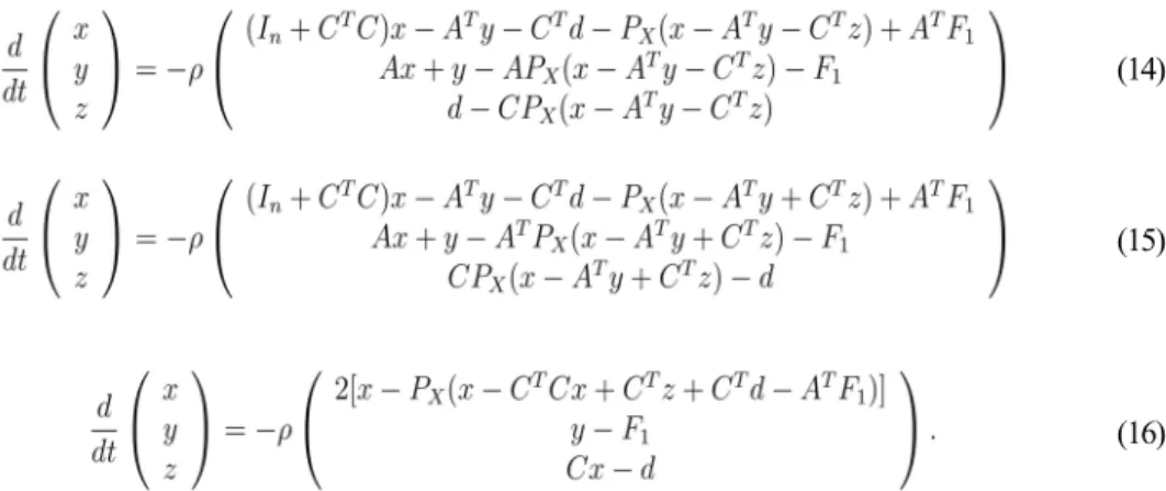
Next, let us focus on the models in [12], [26] and [27], their state equations for (1) are listed as follow
(11)
(12)
(13)
For all of (14), (15) and (16), . Their corresponding output equation are and x = x, respectively. Thus, they all require m + n + p state variables, while (11)-(12) needs m + n state variables. Furthermore, the first two of them both have two-layer and the third one has three-layer, however the model designed by this paper has only one-layer.
Third, let us look at the model in [29], for (1), which can be written in details as and
where and x = PX (x) is the corresponding output equation. Although, (17) has
m + n state variables which is same as (11)-(12), this model is two-layer. More importantly, the stability of this model maybe questionable in some case (see [33]). To guarantee the solution of (17) convergent to the optimization solution of (1), there should be exist a parameter k > 1 such that
is positive semi-definite where F2 is defined in (17) and 0 is the zero matrix with corresponding dimension. Actually, that parameter maybe not exist (see Example 1 in Section 3).
Finally, we compare the proposed model with the model in [33], whose state equations for (1) is
where and are defined in (17). The corresponding output equation is This neural network needs m + n state variables is same as (11)-(12), while it has three-layer. Thus it is more complex than the proposed one.
To see more clearly, we introduce Table 1. Table 1 shows that the proposed model has the fewest state variables and layer in structure.
Table 1. Comparison of related models in layer(s) and required neurons
(14)
(15)
(16)
(17)
2.3 Stability Result
In this subsection, the convergence and stable performance of the proposed model will be studied.
Theorem 1. For any starting point , (11) has a unique continuous solution. (11)-(12) is Lyapunov stable. The output variables and state variables will approach an optimal solution of (1) and a point in , respectively. If , the proposed model is globally asymptotically stable.
Proof: From the first inequality of (2), are non-expansive. So, the right-hand-side of (11) is Lipschitz continuous on . Such, for any , (11) has a unique continuous solution on .
From the assume in Section 1, we know (1) has an optimal solution x*. There exist a such that by Lemma 2 i). From the second inequality of (2), let , we get
by setting we have
let and we obtain
let and , we obtain
Since , then
Now, look at the following Lyapunov function
by (11)-(12), the above inequalities and equality in this subsection. Thus, is non-increasing for all t > 0 and (11)-(12) is Lyapunov stable. Hence the set {η (t) | t > 0} is bounded. The set s{η (0)) which called as -limit of η (t), is nonempty, compact, connected and invariant, and η (t) → S (η (0)) as t→ ∞ (see [1]). Clearly, dV(η, η∗) / dt = 0 for all η ∈S(η (0)). So, x = PX(2x- u) for all η ∈S(η (0)).
For all , let be a unique solution of (11) with over , then from the invariance of . Thus for all t > 0. Since S (z0) is bounded, . The remain proof is so similar like
Theorem 3 in [21], so they are leaved out in here.
3. Illustrative Examples
Four examples will be introduced in this section to illustrate the theoretical results achieved in Section 2 and the simulation performance of (11)-(12). In the following discussion, and . The first example shows that the convergence of (13) and (17) is questionable.
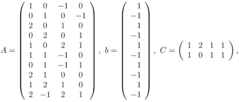
Example 1. Consider problem (1), where , and
Then it has a unique optimal point x* = (0.5, 0, 0, 0.5, −0.5)T .
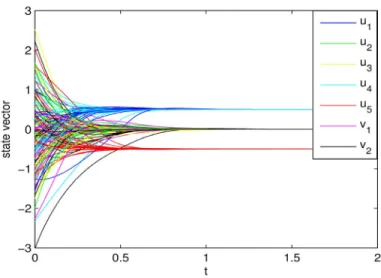
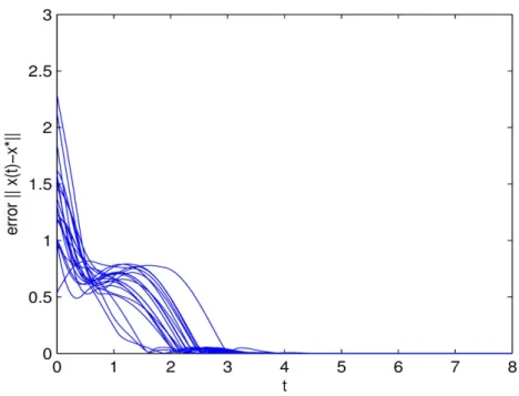
When (11)-(12) applied to this question, all simulation results with different starting points indicate that its state and output variables converge to (u*; v*) and x* respectively. For example, let ρ = 10, Figure 1 shows the convergence of state variables, Figure 2 is the trajectories of output vector, and Figure 3 depicts the convergence performance of ||x −x*||.
Figure 4 shows that the output trajectory of the model (13) with three starting points only converges to (0.125236 -0.0168240.1084110.476629 - 0.280376)T , which is only feasible, but not optimal. The error || x (t
f ) −x*|| = 0.448626. Thus, the model
(13) for this example is questionable.
Consider (17), the AF2 AT in (18) for this problem is
The eigenvalues of AF2 AT are 4.0874 and 1.2526. Thus, for any k ∈ R, the W defined in (18) could not be semi-positive or positive.
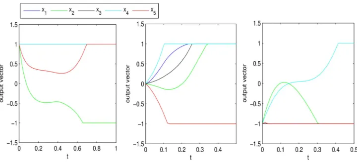
For example, Figure 5 shows that the second component of the output variables of (17) for 07 converges to 1, while for e7 and -e7
to -1; the fifth component of the output variables of (17) for e7 converges to 1, while for 07 and −e7 to -1. Therefore, the convergence of the output variables of (17) is questionable.
Example 2 shows (11) - (12) is better than (14), (15), (16) and (19).
Figure 1. Transient states of (11)-(12) with 20 random initial points in Example 1
Figure 2. Transient behavior of (11)-(12) with 20 random starting points in Example 1
Figure 5. Output trajectories of (17) with e7, 07 and - e7 in Example 1, respectively
Clearly, it has a fundamental solution system as
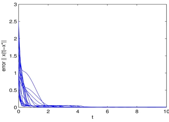
is a free variable. Thus this problem has countless solutions. When (11)-(12) used to solve this problem, all numerical results with different starting points show that its state variables converge to one of equilibrium point and its output variables converge to one optimal solution of (1). Figure 6 shows ||x (t) −x*|| of (11)-(12) with ρ = 10 and 20 random initial points converge to zero.
To compare with the proposed one, (14), (15), (16) and (19) were used to this problem. Their simulation results with three types initial points are listed in Table 2.
Figure 6. Convergence of (11)-(12) with 20 random initial points in Example 2
In there, tfrepresents the time that the stopping criterion, It N denotes the iterative number, || X(tf) − X*|| is the error of output variables, the norm of the right-side hand of these neural network being less than 10-5, is met. Table 2 shows the proposed model
convergence faster than other models.
Example 3 shows the good performances of (11)-(12) in solving general least absolute deviation.
Example 3. Consider problem (1), where X = {x∈ Rn | − 1 < x
i < 1, i = 1, 2, ..., 5}d = (1, −1)T and
We use (11)-(12) to solve this problem. All numerical results show that the state variables of (11)-(12) converge to one of its equilibrium point and its output variables are asymptotically stable at the optimal point, respectively.
Figure 7. Out trajectories of (11)-(12) with 20 random starting points in Example 3
Example 4 shows that (11)-(12) can be applied to solve large-scale problem.
Example 4 [32]. Let A = In, b = 0, (1) is the same as the problem considered by Li i.e. in [32]. Then, (11)-(12) can be applied to solve the Example 3 in [32].
Figure 8. Convergence performance of (11)-(12) with 20 random initial points in Example 3
4. Conclusion
This paper presents a one-layer model for solving least absolute deviation problems including both box and equality constraints. Compared with existing models, the proposed neural network requires the fewest neurons and layers and has good performance. The stability and convergence of proposed one is proved by introducing a Lyapunov function.
Some simulation results verify the good results in theory.
(a) (b) (c)
Figure 9. Images for Example 3. (a), (a1) and (a2) are original images; (b), (b1) and (b2) are blurred images; (c), (c1) and (c2) are restored by (11)-(12)
References
[1] LaSalle, J. P. (1976). The Stability of Dynamical Systems., Philadelphia, PA:SIAM.
[2] Kinderlehrer, D., Stampacchia, G. (1980). An Introduction to Variational Inequalities and their Applications. New York: Aca-demic.
[3] Ruszczynshi, A. (2005). Nonlinear Optimization., Princrton and Oxford, PA:USA.
[4] Bazaraa, M. S., Sherali, H. D., Shetty, C. M. (1993). Nonlinear programming-theory and algorithms, 2nd ed. New York: Wiley.
[5] Wang, Z. S., Xia, Y. S., Chen, J., Cheung, J. Y. (2000). Minimum fuel neural networks and their applications to overcomplete signal representations, IEEE Trans. Fundamental Theory and applications, 47 (8), p. 1146-1159, August.
[6] Wang, Z. S., He, Z., Chen, J. (2005). Robust time delay estimation of bioelectric signals”, IEEE Trans. Biomed. Eng, 52 (3), p 454-462, March.
[7] Wang, Z. S., Peterson, B. S. (2008). Constrained least absolute deviation neural networks”, IEEE Trans. Neural Netw., 19 (2), p 273-283, Feburuary.
[8] Xia, Y. S., Ye, D. Z. (1997). Neural network for solving L1-Norm Minimization Problem “, Acta Electronica Sinica, 25 (11), p 99-103, November
[9] Xia, Y. S., Wang, J. (1998). Neural networks for solving least absolute and related problems”, Neuro- computing, 19, p.13-21. [10] Xia, Y. S., Kamel, M. S. (2007). Cooperative recurrent neural networks for the constrained L1 estimator”, IEEE Trans. Signal Process., 55 (7), p 3192-3206, July.
[11] Xia, Y. S., Kamel, M. S. (2008). A generalized least absolute deviation method for parameter estimation of autoregressive signals”, IEEE Trans. Neural Netw., 19 (1), p 107-118, January.
[12] Xia, Y. S. (2009). A compact cooperative recurrent neural network for computing general constrained l1 norm estimators”,
IEEE Trans. Signal Process., 57 (9), p 3693-3697, September 2009.
[13] Xia, Y. S., Sun, C. Y., Zheng, W. X. (2012). \Discrete-time neural network for fast solving large linear L1 estimation problems and its application to image restoration”, IEEE Trans. Neural Netw., 23 (5), p 812-820, May.
[14] He, B. S., Liao, L.-Z. (2002). Improvements of some projection methods for monotone nonlinear variational inequalities”, J. Optim. Theory Appl., 112 (1), p 111-128.
[15] Liu, Y. W., Hu, J. F. (2016). A neural network for l1 -l2 minimization based on scaled gradient projection: Application to compressed sensing”, Neurocomputing, 173, p 988-993.
[16] Cadzow, J. A. (2002). \Minimum ‘1, ‘2, and ‘1 norm approximate solutions to an overdetermined system of linear equations”,
Digital Signal Process., 12 (4), p 524-560, October.
[17] Hopield, J. J., Tank, D. W. (1986). Computing with neural circuits: A model, Science, 233 (4764) 625-633.
[18] Tank, D. W., Hopield, J. J. (1986). Simple neural optimization networks: An A/D converter, signal decision circuit, and a linear programming circuit, IEEE Trans. Circuits Syst., CAS-33 (5) 533-541, May.
[19] Tao, Q., Fang, T. J. (2000). The neural network model for solving minimax problems with constraints, Control Theory Appl., 17 (1) 82-84. Feburuary.
[20] Avriel, M. (1976). Nonlinear Programming: Analysis and Methods. Englewood Clis, NJ: Prentice-Hall.
[21] Gao, X. B. (2004). A novel neural network for nonlinear convex programming”, IEEE Trans. Neural Netw., 15 (3) 613-621, May. [22] Gao, X. B., Liao, L. Z., Xue, W. M. (2004). \A Neural Network for a Class of Convex Quadratic Minimax Problems With Constraints, IEEE Trans. Neural Netw., 15 (3) 622-628, May.
[23] Gao, X. B., Liao, L.-Z. (2006). A novel neural network for a class of convex quadratic minimax problems, Neural Comput., 18, ( 8) 1818-1846.
[24] Gao, X. B., Liao, L.-Z. (2010). A new one-layer network for linear and quadratic programming, IEEE Trans. Neural Netw., 21, ( 6) 918-929, June.
[25] Hu, X. L., Wang, J. (2007). Solving Extended Linear Programming Problems Using a Class of Recurrent Neural Networks”,
IEEE Trans. Neural Netw., 18 (6) 1697-1708, November.
[26] Hu, X. L.(2009). Applications of the general projection neural network in solving extend linear-quadratic programming problems with linear constraints, Neurocomputing, 72, p.1131-1127.
[27] Hu, X. L., Sun, C. Y., Zhang, B. (2010). Design of recurrent neural networks for solving constrained least absolute deviation problems”, IEEE Trans. Neural Netw., 21 (7)1073-1086, July.
[28] Xue, X. P., Bian, W. (2009). A project neural network for solving degenerate quadratic minimax problem with linear con-straints”, Neurocomputing, 72, 1826-1838, 2009.
[29] Liu, Q. S., Wang, J. (2015). A Projection Neural Network for Constrained Quadratic Minimax Optimization , IEEE Trans. Neural Netw., 26 (11) 2891-2900, July 2015.
[30] Liu, Q. S., Wang, J. (2016). L1-Minimization Algorithms for Sparse Signal Reconstruction Based on a Projection Neural Network”, IEEE Trans. Neural Netw., 27 (3) 689-707, March 2016.
[31] Liu, Q. S., Yang, S. F., Wang, J. (2017). A Collective Neurodynamic Approach to Distributed Constrained Optimization”, IEEE Trans. Neural Netw., 28 (8) 1747-1757, August 2017.
[32] Li, C. P., Gao, X. B. (2016). A new neural network for l1-norm programing”, Neurocomputing, 202,p. 98-103.
[33] Gao, X. B., Li, C. P. (2017). A new neural network for convex quadratic minimax problems with box and equality constraints,