Diffusion in systems with static disorder

(1)

PHYSICAL REVIE%'

8

VOLUME 29, NUMBER 4

Diffusion

in systems with

static

disorder

P.

J.

H.Denteneer and

M. H.

Ernst

Institute for Theoretical Physics, Princetonpiein 5,P.O.Box 80006,3508-TA Utrecht, The Netherlands (Received 28June 1983)

%'e _study diffusion in systems with static disorder, characterized by random transition rates Iw„),which may beassigned to the bonds [random-barrier model (RBM)] or tothe sites [random-jump-rate model (RIM)]. We make an expansion in powers ofthe fluctuations

5„=(to„'

—

(w

')

)/

(w

')

around the exact diffusion coefficient

D=1/(to

')

in the lowfrequency regime, using di-agrammatic methods. Forthe one-dimensional models we obtain asystematic expansion in powers

of Vz of the response function (transport properties) and Green's function (spectral properties}.

The frequency-dependent diffusion coefficient in the RBM is found as Uo(z)=D —, a2V—Dz

+cxoz+a)z

+

'

',

_where _K2=

_{(5 ),}

_cxo_{mcludes lip} _{to fourth-order} _{flllctuatlons} _and

cx)lip tosixth order. In the RJM, Uo(z)

=B.

Similarly, we obtain results (very different in RBMand RJM) for

the frequency-dependent Burnett coefficient Uq(z}and the single-site Green sfunction Go(z) [which determines the density ofeigenstates

M(e}

and the inverse locaHzation length y(e} ofrelaxational modes oftlM system]. The spectral properties ofboth models are ideIltlcal Slid agree with exact re-sults at low frequencies for the spectral properties of random harmonic chains. The long-time behauior ofthe velocity autocorrelation function in RBMisq&

(t)=(

)t

'r~+(

.

)t '~' and for

the Burnett correlation function

p4(t)=(.

~~ _)t

',

_with

coefficients that vanish on a uniform

lat-tice. Forthe RJM,

g2(t)=&6+(t)

and y4(t)=( )t '~

.

The long-time behavior ofthe moments

ofdisplacement (n

),

and

(n4),

and the staying probability Po(t) are calculated up torelative or-der t ~

_.

_A_comparison _of_our _{exact results} _with _those _of_{the effective-medium} _(or hypernetted-chain) approximation (EMA) shows that the coefficient aoin Uo(z) asgiven by EMA is incorrect, contlary to suggestions made ln the literature. Forthe RJM all results can be tlivially extended to

higher-dimensional systems.

I.

INTRODUCTION

Diffusion or hopping conductivity in systems with stat-ic dlsordcr sho%'s lntcrcstlng non-Markovian behavior, which recently received much attention. ' ' A review

of

hopping models was given by Alexander et

al.

' and more recent results can be found inRefs. 2

—

16.

One can assign the static disorder

to

the bonds, as is done in random-barrlcr n1odels ' ' ' ' _oI' _{to thc} _sltcs _{as ls done} _ln

random-jump-rate models.

'

Another class

of

models are exactly solvable one-dimensional stochastic Lorentz models, discussel by van Beijeren,'

'

in which the lattice distances SI'crandom variaMcs.

Here we restrict ourselves to hopping models

of

the random-barrier or random-jump-rate type, described by

a

master equation.

It

is known from approxi-mate ' ' ' ' ' ' _and _exact _theories _{that the}

frequency-dependent diffusion coefficient Uo(z) at low frequencies (z

—

+0) behaves as Uo(z)

=D

—

_,

'tt2v'Dz

+

.

,

where-D=

1/& w '

)

is the exact diffusion coefficient and tr2=&(w '

—

&to '&) &/&w '&

.

The inverse Laplace transform

of

Uo(z) corresponds to the velocity autocorre-lation function

{VACF},

y2(t), which shows the

well-known long-time tail

y2(t)-t '"+

'/

of

diffusion in sta-tionary randoln Q1cdla, such as ln thc d-dlmcnslonal Lorentz gas.

' For

higher-order terms, only approximate results based on an effective-medium approxlmatlon (EMA) have been obtained by Webman and Klafter' with

terms

of

order up to zincluded and by Haus et a/. with terms

of

order _up to z included.

It

has been suggest-ed

'

that the EMA gives exact results to terms

of

order z included.

In this paper we present new results for the asymptotic (low-frequency and long-time) properties

of

hopping models

of

random-barrier or random-jump-rate type, which are based on an expansion in powers

of

the

fluctua-tions

5„=(w

'

—

&w '&)/&w '& around the exact dif-fusion coefficient (see Sec.

III).

The terms in this expan-sion are calculated using

a

diagrammatic method (see Ap-pendix A) and it is shown that this fluctuation expansion is a systematic expansion in powers

of

Vz (see Appendix

8).

In

Sec.

IV we give explicit results for the frequency-dependent diffusion coefficient in the form

Uo(z)=D

—

₂&2vDz

_+ctoz+ct~z

₊

' '

',

_and _for _many _related

functions

of

interest. Our calculations show that the EMA is in fact the hypernetted-chain approximation for the present diagrammatic method and that the EMA results for Uo(z) are already incorrect in terms

of

order z, in disagreement with the suggestions

of

Webman and Kla-fter and Haus et

al.

(see

Sec. IV).

We have also calculated

in

Sec.

IVthe staying probabihty,

Po(t),

and the single-site Green's function Go(z), which determines the spectral properties

of

the eigenmodes

of

the system. The resulting

eigenvalue problem is identical to that for the harmonic chain with random masses or random force constants. Our results appear to be in con1plete agreen1ent arith

(2)

1756

P.

J.

H.DENTENEER AND M.H.ERNST 29

cent exact results

of

Nieuwenhuizen for the density

of

states and inverse localization length

of

eigenfunctions in

aharmonic chain with random masses.

For

a random-jump-rate model, discussed in

Refs.

7 and 25, all results can be trivially extended to higher-dimensional systems, as shown in

Sec.

V, where some

of

the d-dimensional lattice functions are analyzed. In

Sec.

VIwe present abrief discussion

of

our results.

The hopping models

of

interest are described by

a

mas-ter equation

of

the general form

where

p„(t)

represents the probability

of

finding the ran-dom walker (hopping particle) at time t on site n

(n

=0,

1,2,

. . .

,N

—

1)

of

a regular one-dimensional lattice

with periodic boundary conditions _(p»+~

—

_p„)

and lattice distance equal to unity (an overdot denotes a derivative with respect to time). The transition matrix

L„allows

only transitions between nearest neighbors and the transi-tion rates

w„(n=0,

1,

. .

. , N

—

1) occurring in

L„~

are positive time-dependent random variables, with a

site-independent distribution vr(w). The first few inverse mo-ments (w

')

=

w m(w)dw are assumed to exist

0

(I

=

1,2,.

.

. , 6). In this paper angular brackets

(

)

always

denote an average over random variables [w„

I.

We consider two types

of

hopping models, a bond

prob-lexn and asite problem, in which the random variables are assigned to the bonds [random-barrier model (RBM)]and to the sites [random-jump-rate model

(RJM)],

respectively. The master equation for the

RBM

has the explicit form

exact relation in the

RJM

for all times and for general

dimensionality, implying that the VACF gran(t)=D5+(t) [with

f

5+(t)dt=1],

without any long-time tail. How-ever, long-time tails show up in the Burnett correlation function, related to the fourth moment

of

the displace-ment.

II.

PROBABILITIES OF DISPLACEMENT, RESPONSE AND GREEN'S FUNCTIONS

From a macroscopic point

of

view one is interested in

P„(t),

the probabilities

of

displacements n at time tin

a

sta tionary initial ensemble, averaged over the random

vari-ables [w„I [the analog

of

the Van Hove function

G(r,

t)],

which determines most quantities

of

physical interest, such as the transport properties.

Of

particular interest are the lower moments

N—1

(n'),

=

_g

n'P„(t).

n=0

(2.1)

For

instance the diffusion coefficient follows from the long-time behavior

of

the mean-square displacement,

(n'),

=2Dt.

The Fourier transform

of

P„(t)

(the so-called intermedi-ate scattering function) is the generating function for these moments. In our analysis we actually calculate the

response function W(q,z), which is the Fourier-Laplace transform

of

P„(t):

N

—

1

W(q,

z)=

g

e't"P„(z)

.

p» w»—1(p»

—

1 p»

)+»(p»+1

p»)

(E„—

1)w„—

(E„—

1)p„,

(1.

2)

where

E„f„=

_f„+~

and w„denotes the random transition rate for jumps across the nearest-neighbor bond between

the pair (n,

n+

1). The stationary solution

of (1.

2) is a site-independent constant:

Laplace transforms are in general denoted as

F(z)

=

I

e

"F

(t)dt and the reciprocal lattice vector

q=2~l/N

with l

=

—

—,

'X+

1,

.

,—,

'X

lies in the first Brillouin zone

(1BZ).

It

is further convenient to use the orthogonality relations

N

—

1

N

g

e'"'t

't

'=$,

, N

—

'

~

~'e~»—~&

n=0

qG1BZ

(2.3) normalized such that

g„o'

g„=N.

The master equation forthe (isotropic)

RJM

reads

0

I

n wn —1pn —] 2wnpn+wn+1J n+]

=

—

(2

—

E„—

E„')

w„p„.

(1.

4)

Henceforward the limits on the summation signs will be dropped and every sum over sites runs from

n=0

until n

=i%

—

1and all q sums run over the 1HZ.

In generalized hydrodynamics it is often convenient to express the response

function,

~

(q, z) in terms

of

a

gen-eralized diffusion coefficient U(q,z) as Here a random jump rate

v„(or

waiting time

1/v„)

is

as-signed to the nth site and the particle jumps with equal

probability to one

of

it» nearest-neighbor sites. Hence the transition rate for a jump to any nearest neighbor

of

the

nth site is

w„=

—,'

v„.

The stationary solution

of (1.

4) is

g„=

C/w„,

where Cis determined from the normalization condition

g„g„=N,

yielding C '

=

g„(Nw„)

=(w

).

Using the exact diffusion coefficient for this model

D=1/(w

'),

as given by Haus et al., one finds

the stationary solution

of (1.

4) as

.

x

(q, z)

=

[z

+q'U(q,

z)

]

The ordinary diffusion coefficient Dfollows from D

=

lim lim U(q,z) .

z~Oq~O

(2.4)

(2.5)

W(q,

z)=

—

q2

(n

2

)(z)+

—

q

(n

)(z)+

~ ₄ ₄

2 2 4l (2.6)

The Laplace transforms

of

the moments

of

displacement,

(n )(z),

generated by (2.2),

i.

e.,

P„=D/w„.

(1.

5) can be expressed in terms

of

U(q,

z). To

do sowe expand

(3)

29 _{DIFFUSION IN SYSTEMS WITH STATIC}_DISORDER ₁₇₅₇

(n—

')(z)=z

'U, (z)+z

'U',

(z) .

Here Uo(z) is the "frequency-dependent" diffusion coeffi-cient

[Uo(0)=D]

and U2(z) is the frequency-dependent modified Burnett coefficient. The inverse Laplace transforms

of

Uo(z) and U2(z) will be referred to as the velocity autocorrelation function (VACF) q)2(t) and the Burnett correlation function q)q(t), respectively. ' '

In order to relate the macroscopic probability

of

dis-placements to the solution

of

the master equation

(1.

1), we observe that the conditional probability or Green's-function solution

I

„(t)

of (1.

1) with

I

„(0)

=5„equals

the probability

of

a displacement (n

—

m) in afrozen con-figuration

{u)„j,

given that the walker starts at site m. Let

_P~

be the stationary initial distribution (with normali-zation

g

f~=N)

for a frozen configuration

_{w„j,

as

given in

(1.

3) and

(1.

5); then

~„(t)

=

g

r„,

(t)q rN

(2.9)

and use it

to

obtain a similar expression for W(q,

z).

Com-parison with (2.6) then yields

—,'

(n')(z)

=z-'U,

(z),

(2.8)

Lqq

=N

ge

q (E& 1—)io

(E

—

1)e

=f*(q)

~qq

f(q')

=(f*

~f),q,

and in the

RJM

from

(1.4):

Lqq

=f'(q)f

(q)~qq

=(f'f

~)qq

where

Wq«

N—

—

'

g

w„e'"'q

f

(q)=e

'»

—

₁

_.

The Laplace transformation

of

(2.12) reads pq(z)

=

g

Pqq (z)%qq——[P(z)%]qq

q'

where the Green's function is defined as

I'qq(z)=[(z+L)

']qq

The response function can finally be put in the form

P

(q,

z)=(P

(z))

=

y

(I

(z)(P ~

)

q'

=((z+L)-'q

)„.

(2.15)

(2.16)

(2.17)

(2.18)

(2.19)

(2.20)

is the probability

of

a displacement n in a frozen configu-ration _I

_u)„j

averaged over all possible starting positions

of

the random walker. The macroscopic probability

of

dis-placements is then

Note that the response function differs in general from the

auerage Green's function (which is the diagonal element

of

the average

of

the Green's function

I

q»

):

P„(t)=(~„(t))

=N

'g

(I'„(t)g

),

(2. 10) (2.21)

p,

(t)=

ge""~„(t)

. (2.11)

With the help

of

(2.9) and the orthogonality relation (2.3)

itcan be written in the form

where the angular brackets denote an average over the random variables _{

_w„j.

The probabilities

rr„(t)

for a frozen set

of

{io„j

values

do not have the translational symmetry

of

the lattice; however, averages

( )

do have this symmetry. We there-fore introduce the Fourier transform

However, in the

RBM

P

(q,z) and

S(q,

z) coincide since

=1

is the uniform stationary distribution

(1.

3) or equivalently %qq~ 5qq

.

A quantity

of

interest is the density

of

eigenstates.

If

one represents pq(t) by p»(t)

=e»'»"pq

then (2.12) reduces to an eigenvalue problem,

Lp=ep

with solutions _{

e,

_p»

'j

(a

=

1,2,

. . .

,

N).

Using the well known identity

(x

i

0)

'=—

P(1/x)+mi5(x),

w._here

_P

_{denotes the} princi-pal value and

5(x)

the Dirac

5

function, we can write the average density

of

eigenstates per lattice site as

M(e)=N

'g

(5(e

e))—

p

(t)=

QI

(t)%

=[I

(t)%]

q'

where we have introduced

e'q"p _e

'q™

qq'

~

pm

n,m

(q

—

q')

(2.12)

(2.13)

=(mN) 'Im

g

_((e

e i

0)

')—

—

=

—

~-'tm

N-'

_g

_{(( e+L}

₊

i

0)

')—

q

'Im[Gp(

—

e+i

0)] .

(2.22)

Here p»(t) satisfies the transformed master equation:

p»=

—

XL»»

p»

=

(Lp)»

.

—

(2.14)

Here Go(z) is the auerage single site Green's fu-nction de-fined in terms

of

(2.21)through

q'

G„(z)

=N

'

g

e '«"9'(q,z)

.

(2.23)

The transition matrix in the

RBM

can be obtained directly

(4)

P.

J.

H. DENTENEER AND M.H. ERNST

Green's function is the exponential growth rate (inverse

localization length)

y(c) of

eigenfunctions. In one-dimensional cases this concept

'

can be explained by

considering our eigenvalue problem in configuration space

by putting pn(t)

=e

"pn in

(1.

2) and

(1.

4). The transfor-mations

u„=

—,

_w„(p„+I

—

p„)

for

RBM

and

u„=w„p„

for

RJM

map these eigenvalue equations onto

—

Eun

=

w„(un

₊

I

+

u„ I

—

2u„)

.

In this case we doQot use periodic boundary conditions but consider eigenfunctions vanishing at both ends

of

the chain. The solution

uz(c) of

this recursion relation with

Q ]

=0

and Qo

=

1 1sapolynoIMa1

of

degI'ee

X

1Q6»&here

the coefficient

of

{

—

e) isgiven by

+„0

(1/w„).

Let

e„

with

n=0,

1,2,

. . .

,

Ã

—

1 be the (unknown) zeros

of

this polynomial, theQ

X

—

I

uiq{e)=

g

[(c„—

c)/w„]

.

An eigenfunction must vanish at both ends

of

the chain. Since uiv(en )

=0,

the zeros c'n

of

_{uiq(e) are the eigenvalues.}

If

the solutions

of

(2.24) grow exponentially fast, then the large-N behavior

of

y(c)=N

'(ln

~uiq(c) ~

)

with

e+e„

measures the exponential growth rate provided

y(e)

is positive. Inthe thermodynamic limit, where the spectrum becomes dense,

y(e)

can be defined by taking c just above orbelow the real-c axis, so that

equally well to the isotropic

RJM

even for general dimen-sionahty.

We start with the

RBM,

where the average Green's function (2.21)and the response function (2.20) are

identi-cal as explained below (2.

21):

~

—

I

~

_g i (qn—q')

qq'=

~

ne

5„=D(1/w„—

(1/w )

),

(3.

2c)

where W ' is the matrix inverse

of

W as can be verified from (2.17) and (2.

3).

Using amatrix identity wewrite

I

(z)={z+f

8'f)

'=f

'W

'(zW

'+ff

)

'f

where we have used (2.

13). For

z~O

the above functions reduce to

~(qO)=[f(q)l

'(~

'&

_[f'(q)]

'

=

[2D

(1

—

cosq)]

We want to expand the resolvent in the proper fluctua-tions aI'ound their value at

z=O,

y(c)=Re'I

X

'(In[uiq(c+i

0)]

)

I

Pf

—

1

=Re

N '

g

(In[(e„e+iO)—

/w„])

.

(2.25)

=

_f

'(1+6,

)(z+zA+a))

'f,

where wc 11Rvcused (2.17)to wrltc

co(q)

=Df*(q)

f

(q)

=2D(1

—

cosq)

.

(3.

3)

The positivity

of

this function is related tothe exponential

locallzRtloll

of

Rll clgcllfllIlctlolls.

For

our purpose it is moxe convenient to consider

dy /de

Rs lt ls directly related to tllc slllglc-sltc Grccll s function (2.

23):

The function for the

RBM

follows from these equations

W(q,

z)=((1+6)(z+ro+zh)

')qq

.

If

we neglect the fluctuations in

(3.

5)we find the Green's function go(q, z)for auniform lattice with a constant tran-sition rate

D=

1/(

w '

):

go(q,z)

=

[z +co{q)]

(3.

6)

(2.26)

In the following we use the abbreviated _{notation go(q)} for go(q,

z).

In our systematic approach we expand the response function in powers

of

6,

which yields for the RHM,

Here y(0)

=0

since the eigenfunctions with c

—

+0,

i.

e.,the long-wavelength modes with

q~O,

are essentially the same as in the uniform lattice and are therefore not local-1zed.

a

(q, z)

=go(q)

zc0(q)g0(q)A(q,

z—

)

(3.

7)

Our method is a generalization

of

Zwanzig's calcula-tion' for the response function M(q,z) in the

RBM,

which leads to asystematic expansion in powers

of

Wz as

z~O

with q

=avz

and a fixed. The essential point in this calculation is the proper choice

of

fluctuations: Auc-tuations

_{1/w„—(1/w )}

around the exact inverse diffusion cocfflclcnt

D

=(1/w).

Thc nlctllod call bc Rppllcd

(5)

gen-DIFFUSION IN SYSTEMS WITH STATICDISORDER 1759

q'U(q,

z)

=~(q)+r(q,

z) (3.10)

I'(q,

z)=[~(q

z)l

'

—

[gp(q,

z)]

'

eralized diffusion coefficient U(q, z)defined in (2.4) with is identical to the response function

(3.

5) in the

RBM.

The response function

P

(q,z) and the generalized dif-fusion coefficient U(q,z) or

1(q,

z) defined in

(3.

10) can again be expanded in powers

of

b,:

=zto(q)A (q,

z)[1

—

zoo(q)gp(q)A (q,

z)]

(3.11) W(q, z)

=gp(q)+co

(q)gp(q)A (q,

z),

_(3.

₁₄₎

~(q,

z)

= ((z+

f"f

~)

'(

I+&)

_)«

=

₍₍₁₊

6,

)(z+zA+co)

'(1+

6,)

)«

.

(3.

12)

Note that the average Green's function (2.21) for the

RJM

S(q,

z)=((z+f

fW)

')«

= ((1+

b,)(z

+zh+co)

—'

)

_«

(3.13)

For

the

RJM

the response function (2.20) contains the sta-tionary initial distribution

(1.

5),

g„=D/w„

through the matrix

V. It

satisfies

4=1+

b, on account

of (3.

2a). Combination

of

(2.20) and (2.16)gives the response func

tion for the

RJM

in the form

I

(q, z)

= —

co _(q)A _(q,

z)[1+to

(q)gp(q)A (q,

z)]

where A(q,z)is given in (3.8).

In order to calculate the terms in the fluctuation expan-sion

of

A(q, z) we have developed a diagrammatic expan-sion. As the method is rather involved it is presented in a separate appendix, Appendix

A.

The result

of

these calcu-lations, with sixth-order fluctuations included

[i.

e., terms with l

=0, .

.

, 4 included in the definition

(3.

8)

of

A(q,

z)],

is given by the following formula, which is ap-plied toone-dimensional hopping models in Sec. IV and to higher-dimensional ones in

Sec.

V:

A(q,

z)=a2hi

—

z~3hi+z

[~4hi+a~2(gphi+gi+hih2)]

—

z'~2~i(2gphi+3h

~h2+4gihi+hi)

+z

K'z(gph i+2gph igi +2gph ih

2+&

ih3

+h

&h 2

+h2+

3g2h&

+4g3)+

' ' ' _(3.₁₅₎

The functions

_g„(n

=1,

2,3, .

.

.)defined in

(85) of

Appen-dix

8

depend on q and z whereas

h„(z)

and

h„(z),

defined

in

(Bl)

and

(89),

depend only on z. The cumulants

at=((5

)) are given in terms

of

moments

pt=(5')

with

5=D(w

'

—

(w

'))=D/w

—

1. The first few

of

them are given by

K2=P2~ K3=P3~

2

K4

—

p4

—

3p2, K5

—

p5

—

10p3p2,

K6 ——_p6

—

15p~2

—

10p3+

2 30p23

.

(3.16)

%e

have assumed that the _p~ with /

(6

exist.

The main goal

of

this paper is to present a systematic calculation

of

the small-z and -q behavior

of

the response function, in particular for the range

of

_q values with q

of

order aVz (with a fixed) or smaller.

For

the one-dimensional case we have made a systematic analysis

of

the small-q and -zbehavior

of

all terms in the fluctuation expansion, which is presented in Appendix

B.

There it is

shown that

_((zhgp)

_)«

is

of

order

z~'"

with

a(l)

=

—,'

[

—,'

(i

+

_1)] to leading order for small z with

q=ttVz.

The function

_[x]

is the largest integer smaller than or equal to

x.

Hence the perturbation expansion

(3.

15) starts with a term

of

order z '~ in the one-dimensional case and is exact to order

z'

terms included. The contributions to (3.15) from

((bgp)

),

proportional to

K3 K4K2, and K6, should be neglected as they are at least

of

order z[see

(814)].

diffusion coefficient Up(z) and modified Burnett coeffi-cient U2(z), defined in (2.7),at low frequencies, as well as the long-time behavior

of

the moments

of

displacement. We further calculate the long-time behavior

of

the staying probability Pp(t) and the small-z behavior

of

the single-site Green sfunction Gp(z), which describes the density

of

eigenstates

M(e)

and the inverse localization length

y(e)

at the lower end

of

the eigenvalue spectrum.

To

calculate Up(z) and U2(z) we need the _q expansion (2.7)

of

_q U(q,

z)=to(q)+I'(q,

z).

As

I

(q, z) has been ex-pressed in

(3.

11)and

(3.

14) in terms

of

A(q,z),we also in-troduce its _qexpansion:

A(q,

z)=Ap(z)

—

q

Az(z)+

(4.1)

Bycollecting the results

of

Appendix

8

to the relevant or-der in zone finds from

(3.

15)

DAp(z)

=

—,tt2(D/z)'~

+ap+ai(z/D)'~

+0(z),

DA, (z)

=b,

D/z+b,

(D/z)'"+

O(z'),

(4.2) where the coefficients _{at and bt, listed in Table}

_I,

have been expressed in the cumulants

_ai.

Coefficients with

i=0

involve at most fourth-order fluctuations, those with

i=

1

sixth-order fluctuations.

For

the

RBM

the coefficients Up(z) and U2(z), occur-ring in the q expansion (2.7)

of

the generalized diffusion coefficient, can be expressed inAp and A_z with the help

of

(3.

10) and (3.

11):

IV. RESULTS FOR ONE-DIMENSIONAL HOPPING MODELS

Up(z)

=D

+zDA

p(z),

.

U2(z)

=

—

„D

+z[DA2(z)+

—,_~_DAp(z)

—

D2A

p(z)],

(4.3)

From the results

of

the preceding section and

of

Appen-dixes A and

B

one can calculate the frequency-dependent

(6)

P.

J.

H.DENTENEER AND M.H. ERNST

TABLE 1.Coefficients in terms ofcumu1ants.

Qp

Cp

C1

Sp

1 11

—

₄_K3+₂₄K2

1345

TK 16 K2 96K2K3+2304K2

7 2 27K2

29 107

108K2K3+216 K2

1 1

12

+

108

1 3 24K2

—

54K2K3+27

1 1 127 12 2K3+108 K2

1 665 5747 12K2+4K4 432K2K3+ 3456K2

1

( I,+K3

16K2} 15

15

(K2

—

2K4+2K2K3 16 K2}

1 1 2

—

_4K2

—

_4K3+_8K2

1 3 2 7 25 3

16(

—

K2+ 2K3+ 2K4+ 2K2

—

2K2K3+ 16K2)

EMA

1 3

—

_4K3+_8K2

21 3 8K4 16"2 16K2K3+

~

K2

1 4 K2

1 3 3

—

_4K2K3+ _8K2

1

12

1

24 K2

1 1 '2

12

—

2K3+K2

33 12K2+4K4

—

8K2K3+32 K2 16(

—

~+K3

—

4K2}

3 2

1 3

(K2 2K4+K2K3 2K2} exact

16(

—

K2

+

2K3

+

2K4

—

3K2K3

+

₄5K23}

Up(z)=D[1+ ,

'III(z/—D)'

+ap(z/D)

+~I(z/D)'

'+O(z

_)],

UI(z)

=D[cp+ci(z/D)'

+O(z)],

1 L 1

CP

=

12

+bP

—

4K2

1

C)

=6)

—

aPKP+ 24K2

.

(4.5)

walks on uniform lattices, since

&z=D

((Ip

(Ip

'))I)

vanishes. Also the higher corrections, ap

and a1,are vanishing on auniform lattice. The long-time

behavior

of

the VACF _{g &(t)}is given by the second

deriva-o

f

(4.'7).

It

has the well-known long-time t

—'~+

'~ (d is the dimensionahty), typic»

«dif«»o»n

stationary random media, such as the Lorentz gas.

The long-time behavior

of

the fourth moment follows similarly from (2.8),(4.4) and (4.5):

ExpressiolIS

for

cp aIld

ci

1II terms Of cllIIllllalltS ICI a1'e

given in Tab1e

I. For

the

RJM

we obtain similarly from

(3.

10) and

(3.

14)

—

(n4),

= ,

'D

t +(4/—3Vm)»

(Dt)

/

+d,

Dt+2d

i(DI

/It)I~'+0

(tP) (4.8)

Up(z)=D,

Uz(z)

=

—,',

D

+

D

Ap(z)

(4.6) with the coefficients dt defined as

dp

=cp+

20p+

~K2,

dI

—

c

1

+2a

I

+

apiiz,

=D[

2Iiz(D/z)'~

+

—

„+ap+ai(z/D)'~

+O(z)]

.

(4.9)

In the last line

of

(4.6) we have used (4.2). Themost strik-ing difference between (4.4) and (4.6) regarding Up(z) is the occurrence

of a

I/z singularity in the

RBM

and the absence

of

any singular terms in the

RJM,

and regarding

Uz(z) the weaker

~z

singularity in the

RBM

and the stronger 1/Vz singularity in the

RJM.

Next, we consider the moments

of

displacement

(n

)„

which have been expressed in Up and UI in (2.8).

For

the

RBM

the long-time behavior

of

the mean-square displace-ment follows from (2.8) and (4A) as

,

' (n2)t,

=Dt+~&(Dt—/Ir)I~I+ap+ai(~Dt)

(4.7)

To

dominant order the average mean-square displacement is described in terms

of

an effective diffusion coefficient

D=

1/(Ic

')

for

a

corresponding uniform lattice, around which we expand in fluctuations. The second term represents a long-time tail, vrhich is absent in random

and 11sted

I

Table

I.

The above results are also sufficient

to

calculate the fourth cumulant

(&n')),

=&n'),

—

3((n'),

)',

where the leading term behaves as

aIt+

~ for t +a&. The long-ti—me behavior

of (d/dt)((n

)),

=8

(t)

increases proportional to

IIzv

t

as t mao. In a unifor—m lattice this term vanishes

and

8(t)

approaches afinite limit

8(

00)

=D/12,

which is called the super-Burnett transport coefficient.

One sometimes considers' ' _a_modified _Burnett

coeffi-cient Uz(0), which is, according to (4.4), given by

U2(0)

=cpD

in the

RBM.

The Burnett correlation func-tion y4(t), which is the inverse Laplace transform

of

U2(z)„has a

long-time tail y4

t~

with -a coefficient that vanishes on auniform lattice.

In the

RIM

the mean-square displacement, deduced from (2.8) and (4.6),satisfies the remarkably simple form

(n

),

=2Dt,

valid for all times, as was first shown by

(7)

no long-time tail. However, long-time effects caused by

the randomness in the medium, occur in

(n

_},

.

Its

long-time behavior can be deduced from (2.8) and (4.6) and is

given by

—

(n

},=

—,

'D

tz+

~2(Dt)'~z

+(

—,',

+a

)Dt+2a,

(Dt/m)'~

+O(t

₎. (4.10)

The cumulant &&n

"}}

is again proportional to azts~z,

which represents

a

long-time tail, vanishing on

a

uniform lattice. In the IUM the quantities

&(ao)

and UI(0) are divergent due tothe effects

of

long-time tails and the Bur-nett corrdation function y&(t) has a long-time tail

, to bccoIIlpalcd wltll +4(t) t 1I1tllc

RBM.

The probabilities

of

displacement

P„(t)

can also be ob-tained from the small-z, -q behavior

of

the response func-tion

P

(q,z) through Fourier inversion

of

(2.

2).

We are specially interested in the probability

of

zero displacement or staying probability

Po(t)

in case

of

a stationary initial distribution [see (2.10) and (2.

11)].

Its Laplace transform isgiven by

Po(z)=N

'gP

(q,z)

.

(4.11)

Furthermore we are interested in the average single-site Green's function Go(z), corresponding tothe staying prob-ability in case

of a

uniform initial distribution [see(2.

23)]:

Go(z)

=N

'

g

9'(q, z}

.

Go(z)

=h

i(z)

—

zN '

g

to(q)go(q)A (q,z)

.

(413) Bysubstituting

(3.

15)for A(q,z)and introducing the func-tions

k„(z),

f„(z),

and

f„(z),

defined in (B4)and

(Bll)

of

Appendix

B,

we find by including fluctuations up to sixth older

The latter function determines the spectral properties

of

the eigenmodes

of

the system [seeEqs. (2.22)

—

(2.

26)].

In the

RBM

both functions coincide; in the

RJM

they do not. Starting with the

RBM,

where

P

=9

and Po

Go-

—

according

to (3.

1), itfollows from

(3.

7) and

(Bl)

in Appen-dix

8

that

(4.14)

Go(z}=h,

—

zazhlhz+zzaphzihz

—

zi[gc4h

ik2+az(hlkI+

f

I+hihlkz)]+z

alas(2hiki+3h

Ihzkl+4h

if

i+hlkz)

—

z5aI[h

lk4+2hi

fi+2h

Ihzkl

+(h

Ihs+hihz+h2)kl+3hl

fl+4fI

]+

'

+rl(z/D)+O(z'~

_)],

(4.15) wllcrc thc cocfflcfcnts ro and

r

1 al'c listed ill Table

I.

Tllis

result is in complete agreement with the low-frequency behavior

of

the characteristic function Q(z) in a harmonic chain with random masses as determined by Nieuwenhuizen, ~where

Go(z)=dQ(z)/dz.

The a.

t in this

case are cutnulants

of

the mass distribution. In this paper the small-z behavior is determined explicitly up to terms

of

order z ~ included.

It

is used to calculate the specific heat for harmomc chains with random masses. The long-time behavior

of

the staying probability also follows from (4.14) with Go(z)

=Pa(z)

in the

RBM:

P,

(t)=(4~Dt)-'"

—

_(r,

/2v

~)(Dt)-'"+O(t

")

.

-(4.16)

This function is given in full detail as it is also needed in

Sec.

V for higher-dimensional systems. From the small-z behavior

of

these functions as obtained in Appendix

B

we fllld

G

(z}=D

'[

_,

(D/z)'/

_,

K +—r (z/D—)

/—

y(e)

=

_,

'aze/D

+

—,'—r_I

(C/D)2+

0(C3)

.

Po(z)

=hi

(z)+X

'

g

co _{(q)go(q)A (q,}z)

=

Go(z)+E(z),

(4.18)

where Go(z) is the single-site Green's function (4.14), winch also applies to the

RJM

and whele

Using the replica method Stephen and Kariotis ob-tained the same result

for

the density

of

states.

For

the inverse localization length they only obtained the first term on the right-hand side

of

(4.17). The Green's func-tion Go(z) for the

RJM

is identical to the one in the

IBM

by virtue

of (3.

13)and so are the spectral properties. We restrict ourselves to the staying probabihty

Po(t),

which can be obtained from (4.11)and

(3.

14) in the form

and (4.17}

Furthermore, the single-site Green's function Go(z) deter-mines the density

of

eigenstates

~(e)

through (2.22) and the inverse localization length

y(e)

through (2.26). Since Go(z) is known through (4.15)forsmall z, we have for the lower end

of

the spectrum

(a~0):

M(c)

=(2Ir)

'(De)

'~ (ro/Ir)D ~e'~

+—

O(e

~ )

«z)

=&

'

g

~(q)go(q)A (q,z)

.

(4.19)

In deriving

(4.

18) we used the relation t0(q)go(q)

(8)

1762 P.

J.

H.DENTENEER AND M.H. ERNST 29

E(z)

=

~2h)

k)

—

ZK3h )k)

+z

[Kgh,

k)

+K2(hlk2+

f)

+h)

h2k)

)]

—

z

K2K3(3h)h2+h))k)+z

)(2(h)h3+h)h2+h2)kl+

(4.20)

With the help

of

(B12) it results in the following small-z behavior:

E(z)=D

'[

_,

a2(D—/z)'i

+so+s)(z/D)'i

+O(z)],

(4.21)

d

o)(q)=D

g

f*(q,

)f(q

)

a=1

=2D

_g

(1

—

cosq~) a=1

(5.3)

where the coefficients so and s) are listed in Table

I.

The long-time behavior

of

the staying probability follows by adding (4.21)and (4.15) and yields after Laplace inversion

P,

(t)

=

(1+)(.

_,

)(4~Dt)—

'"

-,

=DN

_g

1/w

—

exp[in

(.

q

—

q

')]

.

q q n _W

—

_[(s,

_+r

o)/2M~](Dt)

'~'+O(t

'~'}

.

(4.22)

Itsfluctuation expansion isgiven by

(5.4)

It

is

of

interest to compare the properties

of

both hopping models. The response function M(q, z)to lowest order in z

(with q

=)(v

z and

z

fixed) is the same as in the uniform

chain with an effective diffusion coefficient

D

=

1/(

w '

).

The same holds for the dominant, long-time behavior

of (n

),

and

(n

),

[see (4.7)

—

(4.

10)].

Here, the effects

of

randomness show up in correction terms

of

order V z or 1/V t. The same dominant behavior can again beseen in the staying probability

Po(t)

[see (4.16)]

of

the

RBM.

However, in the

RJM

the fluc-tuations in the random medium increase the dominant, long-time behavior

of Po(t)

in (4.22) by a factor

(1+)(2),

when compared to the staying probability on a uniform chain with effective diffusion

coefficien D

=1/(w

').

V. RJM IN d DIMENSIONS

The results

of

the previous sections can be trivially

gen-eralized to d-dimensional systems for the isotropic

RJM.

Consider a hypercubic lattice with N sites, labeled n, with unit lattice distance and periodic boundary condi-tions. A random jurnp rate v is assigned to the site n, from where the hopping particle jumps to a nearest-neighbor site with a transition rate w

=v

/2d. The

master equation for this model reads

Ena

E-.

a)w-&-a=1 (5.1)

where

E

n

=

n+

e with e a unit vector in the

a

direc-na

tion. Haus et

al.

have shown that the relation

(n~),

=2Dt

with

D

'=(w

')

is valid for all times

if

one starts with the stationary initial distribution. This im-plies the absence

of

long-time tails in the VACF q)2(t).

Nevertheless long-time tails do occur in the fourth mo-ment, as we will see below. After introduction

of

Fourier transforms most steps

of

Secs.

II

and

III

can be reiterated and one obtains forthe response function

[cf. (3.

12}]

W(q,

z)

=go(q)+o)'(q)go(q)a (q,

z),

(5.5)

with A

_(q,

z) defined by

(3.

8) and calculated up to

sixth-order fluctuation contributions included in

(3.

15). The lattice functions h„'"'(z), g„' '(_{q, z),} etc., are the

d-dimensional analogs

of

the corresponding one-dimensional expressions

h„(z),

g„(q,

z), etc. The same applies to the Laplace transform

of

the staying probability, Po(z), given

in (4.18)

—

(4.20). The problem is therefore reduced to an

analysis

of

the d-dimensional lattice functions. Here we

restrict ourselves to the contributions from second-order fluctuations and obtain by virtue

of (3.

15)and (4.1)

A(_q,z)

~()(z)

=~2h') '

(z),

with

h', '(z)

=(2')

_J

I

_dq, dqd[z +co(

q)]

(5.6)

(5.7) The function h') '(z) is the single-site Green's function for a uniform d-dimensional hypercubic lattice with diffusion constant

D

=

(1/w

)

'.

For

two-dimensional square lat-tices ityields

h(P)( ₎ 2

~

4D

~(z+4D)

z

y4D

(5.8a)

where

E(u}

is the complete elliptic integral

of

the first kind. Itsdominant small-z behavior is

h)

'(z)=

—

(1/8vrD)ln(z/4D) . (5.8b)

2

For

a three-dimensional simple cubic lattice h') '(z) is an integral over an elliptic function

K(u)

(Ref. 34) and its small-z behavior is

h)

'(z)=h)

'(0)

(4'

~

)

'Vz-+

.

-

. .

_The _long-time _{tail in} _{the fourth moment} _follows

from (4.6) and (2.8) as

~(q,

)=(( +

W'/D)

'(1+5.

₎₎

=((1+~)(z+o)+«)

'(I+&))--,

(5.2)

(n„),

=4!D [1+)(2H(d)(t)],

dt (5.9a)

where

H (t)

isthe inverse Laplace transform

of

h)(z) (Ref.

1)

(9)

1763 DIFFUSION IN SYSTEMS WITH STATIC DISORDER

H'

'(t)

=[H"'(t)]"=e

'dD'[I,

(2Dt)]d

=(4m.Dt) d~' as

t~~

.

(5.9b)

Here

Io(x)

is a modified Bessel function.

For

the long-time behavior

of

the staying probability we find an expres-sion analogous to (4.22):

P,

(t)=(1+~,

)(4irDt) d~'

.

(5.10)

Analogous results can be derived for the low-frequency behavior

of

the single-site Green's function G (z),which determines the spectral properties

of

relaxational modes in d-dimensional systems.

VI. DISCUSSION

In order to study diffusion properties

of

one-dimensional hopping models we have developed an

expansion in powers

of

the fluctuation

5„=(w„—

(w

')

)/(w

')

around the exact diffusion coefficient

D

=1/(w

),

using a diagrammatic method. This has been done for two types

of

hopping models: the

RBM,

in which the random variables are assigned to the bonds, and the

RJM,

in which they are assigned to the sites.

For

small frequencies

(z~O)

this fluctuation expan-sion is shown to yield a systematic expansion

of

the response function

P

(q,z), and the average Green's func-tion

$(q,

z) in powers

of

vz for small zwith

q-vV

z and v kept fixed. This expansion does not cover the full (q,z) dependence

of

W(q,z)for small qand z. The region where q tends to zero first is not covered by our results, as can be illustrated by calculating

U(0,

z) and U(q,O), defined in (2.4), forthe

RJM.

From (2.7) and (4.6) one sees that

+

'a,

(~D)

'

't

—

'

'+0(t

'

')

(6.4)

1x -' '-

' '

-

'

_&~g2ph31 1X

3 2

2x _+2gp

1x

lim

U(0,

z)

=D

z~O

1X 2X

.

— -' r 3

~ '= = -' +2g_{Og lhl}

X2go1,

Next we obtain from

(3.

12),

(3.

2), and (A3)

1X X'2hlh2 lx ' '

'

'' '= ''= _~~h1h2

A

(q,O)

=

(1+a&)/to(q)

(6.2)

3

X2g2h1

2

1x - -

'

- _~2g1 2x

so that

3 Xgg2hl

&2h1h3

(6.3)

lim U(q,

0)

=D/(

I+@2)

.

q~O

1X -' '& '~ '~

X4h3

3 2X -' -' -' ~ ='

XP

3gph1

r

/ '

~

The transport properties can be obtained from

P

(q, z) [see (2.1)

—

(2.8)] and the spectral properties from

S(q,

z) [see (2.22)

—

(2.

26)].

The difference between

P

and

9'

is the following: In the definition (2.20)

of

P

(q, z) occurs an average over all

starting positions

of

the hopping particle with a weight

function

_g„,

that is the stationary solution

of

the master equation

(1.

1)for a frozen set

of

random variables

Iw„).

This equilibrium weight

P„may

depend on the site label n, as is the case in the

RJM.

In the definition (2.21)

of

9(q,

z) the possible starting positions

of

the hopping par-ticle are given an equal weight.

The frequency-dependent transport coefficient Uo(z}for the

RBM

is given in (4.4). The leading contributions

Uo(z)=D+

—,a2(Dz)'~

+

have been obtained before

by exact calculations, ' by the effective-medium approxi-mation (EMA),

'

by renormalization-group methods, and by mode-coupling theories. The higher-order terms

2x 3

X2g3

1x

K2X3g, h,

X2g33

/

2X X2X3g1h1 2x

1X X.3_2g3

/

1x

X~h2 ~2+3hlh2 1x

2x

'

~ 2 4

X3gPh1

X2X4gPh1

X2X3h1 1x

1X

etc.(9more)

1X -' '~ &' " -' X5h1 1x

etc.(14more)

X6h15

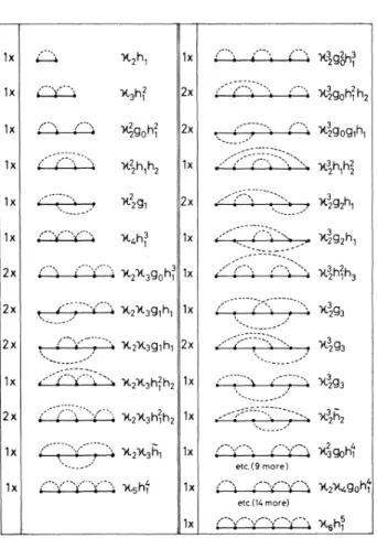
FIG.

1. Diagrams representing the terms ((Ago}'b,

_)«

in the fluctuation expansion (l

=1,

2,.

.

.,5).

in

(44) of

order zand

of

order z arenew results.

There exist approximate calculations based on the EMA

by Webman and Klafter' to order z and by Haus et

al.

to order z

~,

which differ already in terms

of

order z from the exact results (4.4), contrary to the suggestion made in Refs. 8 and

10. For

our comparison with the terms

of

order z / we have used the results

of Ref.

8,'in which clusters containing three sites have been used in-stead

of

the lower approximation

of

two-site clusters.

It

appears that the approximate EMA results are completely accounted for by the contributions from diagrams in

Fig.

1,that are built as series-parallel circuits

of

the first dia-gram element (the so-called hypernetted-chain diagrams), their analytical contributions can be simply expressed in the contribution

hi(z) of

the first diagram (see Appendix A). The diagrams in

Fig.

1, whose contribution contain

g„(q,

z)(n

)

1)or

h„(z)

(n

)

1), do not have a series-parallel structure. The EMA is therefore the hypernetted-chain (HNC) approximation ' i

_of

_{our diagrammatic} _method.

Table

I

gives the EMA values together with the exact ones

of

all coefficients appearing in Sec.

IV.

(10)

P.

J.

H. DENTENEER AND M.H.ERNST

The first term represents the well-known long-time tail

qtz-t

' + '/

_of

_diffusion _{in stationary} _random _media,

such as the d-dimensional Lorentz gas. ' Note that the long-time tails are absent in random walks on uniform lat-tices, where a11cumulants xI are vanishing.

The corresponding mean-square displacement for the

RBM

is given in (4.

7). For

the

RJM

we recover the exact results

(n

),

=

2Dt and qt2(t)

=D5+(t)

of

Haus et

al.

The results (4.4)for the frequency-dependent (modified) Burnett coefficient Uz(z) in the

RBM

are new. The

lead-111gloilg-tin1c tail 1111ts iilvcl'sc Laplace tiailsfor111, whicll is the Burnett correlation function y&(t), behaves as t with a coefficient depending on sixth-order fluctuations. The closely related moment

(n

_),

is given in (4.8). The HNC diagrams reproduce again the EMA results

of Ref.

10for

(n

)„and

the EMA values

of

the coefficients to-gether with the exact ones can befound in Table

I. For a

discussion

of

the EMA results it is more instruc-tive to make the following observation.

If

we denote Uo(z} as calculated from the EMA by W(z), then inspec-tion

of

the structure

of

the diagrams in

Fig.

1 shows that

U(q, z) in the EMA is given by

co(q)8'(z)/D,

so that the response function W(q, z)

=

[z+co{q)

W(z)/D]

'.

In the EMA all quantities derived from the response function (transport coefficients, correlation functions, and mo-ments

of

displacement) are completely determined by the frequency-dependent diffusion coefficient

W(z).

A simi-lar approximation for the Lorentz gas has been proposed by Alder and Alley, and Ernst and van

Beijeren"

have shown, using a diagrammatic analysis, that the contribu-tions neglected in Alder and Alley's approximation are

of

the same type as in the

EMA.

The Burnett functions for the

RJM

behave again very

differently from those

of

the

RBM,

as can be seen by comparing Uz(z) in (4.4) and (4.

6).

The same result for the dominant contribution to Uz(z) in the

RJM

has also

been obtained from the mode-coupling theory, and from renormalization-group methods. Also the probability

of

zero displacement or staying probability Po(t) behaves quite different in

RBM

and

RJM

[cf.

(4.16) and (4.

22)].

The average Green's function determines the spectral properties, which are the same in both models

[cf.

(3.

1)

and

(3.13)],

and also identical to the spectral properties

of

harmonic chains with random masses or random spring constants.

'1

This can be seen by replacing the eigenvalue

c

in (2.24) by cu

.

In fact, the master equation

{1.

2)for the

RBM

describes, after _replacement

of

_{p„by p„,}

the lattice dynamics

of

a harmonic chain with random spring con-stants

_Iui„I.

The eigenvalue problem in lattice dynamics

is obtained by the rePlaceinent Pn(t)

=e'"'Pn.

Our results (4.17} for the low-frequency behavior

of

the density

of

states

~{@)

and for the inverse localization length

y(c)

(see

Sec. Il)

are the same as the recent exact result

of

Nieuwenhuizen, obtained by entirely different methods. In

a

separate publication we have also considered a fluctuation expansion in bare fluctuations

5„=

(urn

—

_(ui)

_{)/(ui )}

for the

RBM,

which provides a systematic method

to

describe the large-z behavior

of

response and Green's functions. Comparison

of

the exact results

of

Uo(z) with the corresponding EMA result shows again

that the EMA accounts only for the hypernetted-chain di-agrams.

The bare fluctuation expansion for the average Green's function gives also a simple method to determine the mo-tnents

of

the areratts spectral density,

f

dee"M(ei

in hopping models or in random harmonic chains, in com-plete agreement with the results

of

Domb et

al.

7

_For

_the

IUM the results have been extended to higher-dimensional systems.

ACKNO%I EDGMENT3

want to thank

T.

M.

Nieuwenhuizen and H. van Beijeren for clarifying discussions.

APPENDIX A

X

ff

go(q;),

whcl'c +»» rcplesciits thc fillctllatioii

~

—

i

g

5

ein(»

—

»')

W (A2)

and the random variables

5„=D

(1/ui„—

(

I/ui

)

=D/w„—

1 with n

=0,

1,

. . .

, N

—

1 are distributed in-dependently.

It

can be represented by diagrams consisting

of

(l+2)

/inc segments,

',

labeled with a wave

number q;

E

Iq,qi,

.

,qi,

q'I,

and

(l+1)

vertices,

, labeled with a site label n;&In&,

. . .

,

nt+ij

and separating the line segments, and

of

dashed lines

"'

_of

_{connecting vertices with}

equal site labels. The contribution

of a

diagram is determined _by the

fol-lowing diagram rules:

J'

(1)

a

factor%

'5„e'"'»»'for

each (2)

a

factor go(q) for each

(3}a

5„„

for each

(4)sum over all internal _q;;

(5)sum over all n;, excluding those terms where uncon-nected n; are equal;

(6)average over all random variables

5„.

An important stat1st1cal concept ln the cRlculat1on 1s

that

5„'s

are independent random variables. This implies that averages

of

the form

_(5„,

_{5„5„, .}

₎

are only

non-vanishing

if

each label occurs at least twice, since

(5„)

=0.

Therefore, each vertex must be connected with at least one other vertex through

a

dashed line.

If

the site

1Rbel Pl 1s connected

to

I

other vertices, lt contributes a

factor

(5„)

=

p,

independent

of

site n

In this appendix we develop

a

diagrammatic method for calculating the fluctuation expansion A(q,z) defined in (3.8). The (l

—

1)th term in the expansion

of

go(q)A (q,z)

isapart from a factor (

—

z) equal to

[cf.

(3.7) and

(3.

8)]

(go(~go)'")»»

=

go{q)go{q')

«»»,

~».

.

."

~»,

')

(11)

As an example consider the term

of

second order in the fluctuation,

&go(~go) )qq' ',

q,

=le

g g

e '

'e

'

_5„,

_„,

_&5„,

_5„,

)go(q)go(ql)go(q')

=go(q)go(q')5„pzhi(z»

Tllcfourtll-order tcrnl,

&go(~go

}"

_&qq

Lg 4/

r

f 7

/

(A4)

Ill tile fll'sf, teITll nI

—

nz n3

—

n—

—

4 or symbolically (1234),

in the next term n_I

—

_nz+n3

n4 or (12—

—

)(34) and similarly we have

(14}(23)»d

(13)(24). The first term is simply

glveIl by

(1234)

=go(q)go(q')5qq p~h I(z)

.

(A6)

Next consider as an example the last term in (A5).

(13)(24)

=-_{go(q)go(q')pz&}

'

g

go(qi)go(qz)go(q3)e"

Pl₎Qtl2

(A7a)

q

=n

i(q

—

qi+qz

—

q3)+nz(ql

qz+q3

q)

—

.

—

The restricted double sum

(ni&nz)

in (A7a) is split into an unrestricted double sum minus a single sum (ni

—

nz)

yielding

(E

5qq q +q E)5qq'. Usillg dc—flnltloll

(85)

this term yields

(13)(24)=go(q)go(q')5„v

zlgi(q

z}

—

h

i(z}1.

Similarly we find

(AS)

(12)(34)

=go(q)go(q')5„p'[go(q}h'(

)

—

h'(

)1

(A9)

(

14)(23)

=go(q)go(q'}5qq pzfh

i(z}hz(»

—

h

i(»1 .

Using the cumulants

(3.

16)the terms (A6), (AS), and (A9)

cRQbecombined 1Gto

where (2.3) and

(81) of

Appendix

8

have been used. .

Ob-serve that matrix elements & _)qq are diagonal on account

of

translational invariance.

The third-order term, becomes similarly

&go ~go)')qq

---

=g,

_(q)g,

_(q

}5„.

_p,

h',

(z).

We may therefore modify the diagram rules and assign

a

value «4h I to the first diagram in (A5) with four

connect-ed vertices, and values «zgohi, «zh, hz, and Kzgi

to

the

second, third, and fourth diagrams, respectively, with two pairs

of

connected vertices. In general we assign to each set

of

j

connected vertices a weight, given by the

jth

cu-Illulallt Kl

.

The number

of

independent q; variables in the modified

diagrams can be determined by observing that the total wave number is conserved at each vertex,

i.

e.,

if

we assign wave numbers to solid lines and dashed lines, the sum

of

incoming q's equals that

of

outgoing q's. Consequently, each term ill & _)qq lsP10Portlollal 'to 5qq .

The diRgrRrrl coIltributloIls RIC Ilow cRIIcU1Rtcd

Record-ing to the modified diagram rules:

(1)label external lines with wave _{vector q; label internal} lines such that the sum

of

incoming wave numbers equals the sum

of

outgoing wave numbers;

(2)a factor go(q) for line _{segment q;}

(3)sum over all independent internal q's with a weight (4) a factor

g".

_z(KJ)

'

for a diagram with mI.

(j

=2,

3,

. . .

)sets

of

j

connected vertices.

Next we consider fifth- and sixth-order fluctuations. The fifth-order terms are symbolically denoted as (12345) (one such term) and (12)(345), (13)(245), (14)(235), (15)(234), (123)(45), (124)(35), (125)(34), (134)(25), (135)(24), (145)(23)(ten such terms), or by corresponding diagrams (see

Fig.

1),where all diagrams are listed as well Rs the correspoIldiIlg R11Rlytic cxpressioIls RIld the molti-plicity

of

each diagram. The subtracted terms in the 10 terms

of

type (

)(")

contain factors p3pzhi(z}, that

can be combined with the contribution

_p5h,

(z) from (12345) to yield the modified diagram, containing cumu-lants instead

of

moments p.k, represented by

go(q)«5h I

.

The remaining contribution

of

(

)(")

can becalculated

directly from the modified diagram rules. As an example consider (135)(24),

&go(~go }'&qq

=

go(q)g'o(q'}5qq

X[«ghI+Kz(goh I

+

hIh3

+g

I

)]

.

(A10)

r

/

q q i'

q&~82

Ego(qi)

_X

go(qz)go(q3)go(qi

—

qz+q3}=«z«3go(q)&

I@go(qi)gl{ql,

z)=«z«~oz(q)hl(z),

(A12)

q1 g2) g3

(12)

P.

J.

H.DENTENEER AND M.H.ERNST

(go(Ago)

}

=go(q)

I~511,(z)+Ii21~2[2go(q)hi(z)+3h

i(z)h2(z)+4III(z)gl(q,

z)+hi(z)]}

. The function II2(z) is defined in

(Bl).

The calculation

of

the sixth-order term is much more involved. We shall only illustrate how the subtracted terms re-sulting from the restricted n; summations may be combined with other terms to yield the modified diagrams. Consider the following terms calculated according to the original diagram rules:

(123456)

=p6goh

i,

(12)(3456)=p2iu4go(go& i

—

hi)

(123)(456)=Plgo(gob

i

—

II i

),

(A14)

(12)(34)(56)

=P2g0(ggh i

—

2giih i

—

h

iII2+2II

i )

.

With the use

of

the definition

(3.

16)

of

the cumulant a.

6the last terms on each line, proportional to hI,can be combined into a modified diagram (123456)with a value I~6hohi, as there are 15 terms

of

type

(")(

.

), 10

of

type (

.

)( - ),

and 15

of

type

(")(.

*)(").

A more detailed comparison

of

terms enables us to combine ~M~~oh I with those

of

type

(")(")(")

to obtain the modified diagram (12)(3456)with a value Ii2&4goh

i.

In this way one finds that the first term on each line

of

(A14)represents the contribution according

to

the modified diagram rules, provided all moments HAMI are

re-placed by cumulants

xi.

As an example we give the modified diagram contribution from (15)(23)(46),

X

go(qi)go(q2)go(q

—

qi+q2)

+go(q2)=a2g2(q,

z)h,

(z),

where

(85)

has been used. The total contribution

of

the sixth-order fluctuation terins gives finally (seealso

Fig.

1):

&gO(~gO)'&

=

gO&Z(gOh

i+2gohlgi+2gO~

iI

2+3II Ig2+4g2+~

ihl+I

ih2+h2)

+go+3(goh I

+4h

Igi

+2~

1~

2+2h

l~1+g4)+go+2+4(2go~ I

+6

Ilg1

+4~

ih2+

3h1 I1)+go+6II1 (A16)

All functions have been defined in

_{(Bl), (85),}

and

(89),

ex-cept

gO(ql)gO(q2)gO(ql)go(q4)

g)pe+~_p)4

&&go(q

—

_qi+q2

—

_q&+q4)

.

(A17) The notation is systematic in the sense that all functions g;(q, z) with i

=1,

2,

.

_,

represent contributions from "self-energy" diagrams that depend on the external wave IluIllbcl _{q, wllcl'cas} tllc lclllailllllg contributions h (z) alld

h;(z) (i

=1,

2,

. . .

,) are independent

of

q. The simplest

q-dependent self-energy diagram is the fourth one in (A5) with acontribution _~2gi _(q,

z).

Also note that the diagrams whose contribution does not contain the function

_g„

(n

)

1)or

h„(h

)

1)are built as series-parallel circuits

of

the very first diagram. These diagrams will bereferred to as hypernetted-chain diagrams. Their contributions can be expressed as products (of powers)

of III,

II2,h3,

. .

.

, where

_II„~

i

—

(

—

1)"h i"

/n!

(n

)

0) [see

(81)

and

(82)]

and the superscript on hi denotes the nth derivative with respect to z.

A.PPENDIX

8

Thc cRlculRtlon

of

fhc scparafc terms in thc fluctuation expansion presented 111AppcIldix Ais in facf,independent

of

flicnulllbcl'

of

dimensions. The behavior

of

these terms for small zand small _{q will} strongly depend on the dimen sionality

of

the system.

In this appendix we define the functions appearing in

II,(

)=&

'+go(q),

n

=1,

2,

. .

.

,

with go(q)

=

[z

+

~(q) ]

and

~(q)

=

2D (1

—

cosq). From

(81)

we have

(81)

II,

(z)=(i

—

II) 'Il„'

_l(z),

_n

_=2,

_3,

_.

The prime denotes dlffclclltlatloll wltll rcspcct to z. On account

of (82)

all these functions can be derived from &I(z). In the thermodynamic limit

(X~oo)

the sums with

qc18Z

may be replaced by

inte-grals (2ir) I

f

dq

.

, and the function &I(z) reduces toan elementary integral:

III(z)

=(2ir)

'

J

dq[z+2D(1

—

cosq)]

=

[.

_(.

+4D)]-'"

.

(83)

Arelated set

of

functions is

I

Appendix A and in the results quoted in Sec.

III,

and we will calculate them for the one-dimensional case. When possible we give exact expressions, otherwise we determine tllc doIIllllallt slllRll-z bcllRvlol _{wlfh q}

=Icv

z alld Ic kept fixed, which issufficient for our applications.

In the remaining part

of

this appendix we present a power counting argument to estimate the leading small-z behavior

of

all terms in the diagrammatic expansion. These arguments are given for the one-dimensional case, but can be extended togeneral dimensions in

a

(13)

k„(z)=N 'go)(q)go(q),

n

=1,

2,

.

. .

Because

(82)

is also valid for

k„and

k)(z)

=

I

—

zh) (z) all

k functions can be derived from h)

(z).

The next set

of

functions

to

be defined is

_g„(q,

z) (n

=1,

2,

3),

with

g)(q,

z)

=N

'

g

go(q) )go(qz)go(q

—

q)+q»

gz(q»)=N

'

g

go(q))go(q2)go(q

—

q)+q2)

g3(q z) N

y

go(q))go(q2)go(q 3)

Xgo(q

—

q)+q3)go(q

—

q2+q3)

.

The function

_g,

(q, z) can be evaluated exactly by transforming the integration variables according to