HYPOSPADIAS AND PRENATAL EXPOSURE TO ATRAZINE VIA DRINKING WATER: A GEOGRAPHIC ANALYSIS
Jennifer Winston
A dissertation submitted to the faculty at the University of North Carolina at Chapel Hill in partial fulfillment of the requirements for the degree of Doctor of Philosophy in the Department
of Geography.
Chapel Hill 2014
ABSTRACT
Jennifer Winston: Hypospadias and Prenatal Exposure to Atrazine via Drinking Water: A Geographic Analysis
(Under the direction of Michael Emch)
This dissertation uses a disease ecology framework to investigate the etiology of hypospadias, a relatively common birth defect affecting the male genitourinary tract. It begins by considering the spatial distribution of hypospadias in North Carolina and whether that spatial distribution can be explained by either compositional or contextual risk factors. It then focuses on a potential contextual risk factor of interest: atrazine, one of the most widely used herbicides in the United States. An endocrine disruptor, atrazine breaks down slowly in soils and water, suggesting that mothers could be exposed to atrazine via contaminated drinking water.
ACKNOWLEDGEMENTS
I owe a debt of gratitude to many people for their support and assistance in the writing of this dissertation. I would like to thank my adviser Mike Emch as well as committee members Tom Luben, Bob Meyer, Larry Band, Melinda Meade, John Florin for their mentorship,
guidance, and flexibility. I would also like to thank my colleagues Veronica Escamilla, Carolina Perez-Heydrich, Mark Janko, Carmen Cuthbertson, Ashton Verdery, and Brandon Wagner for their advice, encouragement, and senses of humor.
I would like to acknowledge the Carolina Population Center for training support (T32 HD007168) and general support (R24 HD050924). I am also grateful to Wesley Stone, Robert Gilliom, Paul Stackelberg, and David Wolock from the US Geological Survey for generously sharing output from their atrazine models.
I am grateful to Merna and Vern Winston and to Ed and Barbara Fuller for both logistical and moral support, without which this work most certainly would have been completed. Finally, I would like to extend a special thank you to Eddie, Henry, and Jack Fuller for their love,
TABLE OF CONTENTS
LIST OF TABLES ... viii
LIST OF FIGURES ... ix
LIST OF ABBREVIATIONS ... x
CHAPTER 1: INTRODUCTION ... 1
Background ... 1
Theoretical Approach: ... 4
Conclusion ... 7
CHAPTER 2: A GEOGRAPHIC ANALYSIS OF COMPOSITIONAL AND CONTEXTUAL RISK FACTORS FOR HYPOSPADIAS BIRTHS ... 8
Introduction ... 8
Methods... 10
Results ... 12
Discussion ... 19
CHAPTER 3: USING GEOGRAPHIC CLUSTERING TO GENERATE HYPOTHESES ABOUT HYPOSPADIAS ... 21
Introduction ... 23
Methods... 24
Results ... 30
Discussion ... 35
CHAPTER 5: SELECTING AN EXPOSURE METRIC TO EXAMINE A RELATIONSHIP BETWEEN ATRAZINE AND HYPOSPADIAS ... 39
CHAPTER 6: HYPOSPADIAS AND MATERNAL EXPOSURE TO ATRAZINE ... 41
Introduction ... 41
Methods... 44
Results ... 49
Discussion ... 57
CHAPTER 7: CONCLUSION ... 59
Study Limitations: ... 60
Directions for further research: ... 61
LIST OF TABLES
Table 2.1: Descriptive statistics for hypospadias cases and controls ... 13 Table 2.2: Compositional risk factors retained by backward stepwise logistic
regression model for hypospadias in North Carolina, 2003 – 2005. ... 15 Table 2.3: Results of logistic regression model including compositional and
contextual risk factors for hypospadias in North Carolina, 2003 – 2005. ... 16 Table 4.1: Distribution of continuous exposure metrics ... 32 Table 4.2: Pearson correlation coefficients between continuous exposure
metrics assigned to women who delivered a baby in North Carolina (N) ... 32 Table 4.3: Comparison of categorized watershed modeling metric and binary
monitoring metric... 33 Table 4.4: Comparison of categorized county metric and binary monitoring metric ... 33 Table 4.5: Comparison of categorized watershed modeling and county metrics ... 33 Table 4.6: Comparison of crude risk estimates from continuous scale exposure
assessment metrics ... 34 Table 4.7: Comparison of risk estimates from categorized exposure assessment
metrics ... 35 Table 6.1: Characteristics of NBDPS hypospadias cases and controls with estimated atrazine exposure, 1998-2005 ... 50 Table 6.2: Distribution of estimated atrazine in water supply and estimated
atrazine consumption ... 52 Table 6.3: Association between atrazine and hypospadias in the National Birth Defects
LIST OF FIGURES
Figure 1.1: Disease ecology triangle describing risk factors for hypospadias ... 4 Figure 2.1: Local spatial autocorrelation of hypospadias cases and model
residuals in North Carolina 2003-2005. ... 18 Figure 3.1: Distribution of soybean production in North Carolina, 2007 ... 22 Figure 4.1: Map of exposure metrics in North Carolina. Panel A illustrates
the county metric; Panel B illustrates the monitoring metric; Panel C illustrates
the watershed modeling metric. ... 31 Figure 6.1: Illustration of possible mechanism for atrazine to prevent
testosterone from binding to the active site of androgen receptor. Panel A illustrates a cross-section of the androgen receptor including the mouth and channel leading to the testosterone binding site. Panel B illustrates atrazine
blocking the mouth of the channel leading to the active site. ... 43 Figure 6.2: Illustration of assignment of atrazine concentrations to water intakes
for public water utilities in Texas. Panel A illustrates WARP stream estimates and concentrations assigned to surface water intakes. Panel B illustrates USGS
LIST OF ABBREVIATIONS
AIC Akaike Information Criterion
CDC Centers for Disease Control and Prevention
CHEEC University of Iowa Center for Health Effects of Environmental Contamination
MRL Maximum Residue Limits
NBDPS National Birth Defects Prevention Study
NCBDMP North Carolina Birth Defects Monitoring Program
OR Odds Ratio
US EPA United States Environmental Protection Agency USGS United States Geological Survey
CHAPTER 1
INTRODUCTION
Background
Hypospadias is a relatively common congenital urinary tract defect affecting between 4 and 6 per 1,000 male infants (1). It is characterized by having the opening of the urethra located on the underside of the penis (2), and surgery is often needed to reposition the urethral opening. Left untreated, hypospadias can lead to difficulty in using a toilet, as well as sexual and fertility problems in adults (3). Hypospadias is believed to have a multifactorial etiology where both genetic susceptibility and environmental exposures may play a role (4).
Disease Ecology
Disease ecology is a medical geography theory that posits that population, behavior, and environment all play a role in determining disease outcomes (5). In fact, most risk factors for hypospadias can be organized into these three categories.
Population level risk factors for hypospadias include maternal characteristics including maternal health, parity, and genetics. Among maternal characteristics, untreated hypertension (6-8), thyroid disease (9), and diabetes (10) all seem to lead to higher risk. There is some evidence that maternal nutritional status may play a role, with certain vitamins (B12, choline, and methionine) perhaps reducing risk (11). There is conflicting evidence regarding maternal BMI, with Carmichael et al (12) finding greater risk amongst mothers with a BMI above 26, but with Adams et al (13) finding no evidence of an increased risk. Risk also increases with age (10, 14, 15), and is also highest among whites (10). First-borns are at a higher risk than higher-parity children (12, 16). Genetics also likely plays a role, as boys with a family history of hypospadias are also more likely to be born with the defect (17).
Behavioral factors include maternal use of progestins (18) and other assisted reproductive technology (17), which seem to increase risk. Fathers in certain occupations, including forestry and logging workers, firemen, policemen, guards, and vehicle manufacturers, may also be at an increased risk (19).
Supporting this hypothesis, Fernandez et al (21) and Giordano et al (22) find a relationship between urogenital defects and endocrine-disrupting chemicals, as well as to maternal occupational exposure to agriculture. Similarly, Brouwers et al (17) find that paternal exposure to pesticides increases hypospadias risk. The pathway for this exposure is not clear, but it may include maternal exposure via seminal fluid (1). Winchester et al. (23) find that 22 birth defects, including genital defects, are more likely to occur in live births with a last
menstrual period during the time of peak annual agrichemical use. Rocheleau et al (24) also find evidence of a modest link between hypospadias and pesticide exposure, although a later study led by Rocheleau finds no association between occupational exposure to pesticides and hypospadias (25). There is also weak evidence of increased risk associated with proximity to landfill sites (26, 27).
Figure 1.1: Disease ecology triangle describing risk factors for hypospadias
Theoretical Approach:
Neighborhoods and Health Framework
A neighborhoods and health framework suggests that the geographic distribution of a disease may be explained by the composition of the people who live in a place or by the context, or the unique environment, of a place (28, 29). Within disease ecology theory, this dissertation therefore uses a neighborhoods and health framework to investigate the spatial distribution of hypospadias, as well as the factors that might lead to that distribution. In the context of this dissertation, the population and behavioral risk factors for hypospadias identified above can be considered compositional effects, while the environmental risk factors can be considered contextual effects.
The first question examined by this dissertation therefore asks how hypospadias clusters in space. It then draws upon the neighborhoods and health framework to control, to the extent
Population:
Maternal health: untreated hypertension + thyroid disease + BMI +/?
Maternal nutritional status (Vitamins B12, Choline, Methionine) -
Maternal characteristics: age; white race + Parity: first born +
Genetics: family history +
Behavior:
Progestins and Assisted reproductive technology +
Paternal occupation: forestry and logging workers, firemen, policemen, guards, and vehicle manufacturers +
Environment:
possible for compositional effects. Any remaining unexplained variation will suggest that contextual effects are playing a role in the geographic distribution of hypospadias.
Watershed Modeling
To help identify what these contextual factors might be, this study uses a number of exposure estimation techniques, including watershed modeling. These models can be used to estimate contaminant concentrations in groundwater and streams when continuous monitoring data is unavailable. Root et al (31) was one of the first to incorporate watershed modeling into a medical geographical study of birth defects by considering whether gastroschisis risk was influenced by maternal residence downstream from textile mills. This dissertation builds upon that work via a novel adaptation of two hydrological models developed by the US Geological Survey (USGS) to estimate contaminant concentrations in groundwater and drinking water. It also compares the estimates provided by these models against water quality sampling conducted by the US Environmental Protection Agency (EPA), as well as data about pesticide use at the county level. It then compares the strengths and weaknesses of using these exposure estimation techniques to predict hypospadias risk.
This dissertation focuses on the potential environmental risk posed by exposure to
groundwater, exposure from contaminated wells or public drinking water supplies fed by these sources is possible.
Some animal studies suggest that atrazine may be associated with genitourinary malformations in frogs at concentrations as low as 0.1 parts per billion (33), although the US EPA concluded in 2007 that atrazine does not adversely affect amphibian gonadal development (32). In human studies, Meyer et al (36) find no statistically significant association between atrazine and hypospadias in their study of agricultural pesticides in eastern Arkansas. On the other hand, the Agency for Toxic Substances and Disease Registry (35) notes that maternal exposure to atrazine in drinking water has been associated with a number of adverse birth outcomes, including urinary system defects.
This dissertation will draw upon two watershed models in estimating maternal exposure
to atrazine via drinking water: Stone et al’s 2013 watershed regressions for pesticides (WARP)
models for predicting stream concentrations of multiple pesticides (37) and Stackelberg et al’s
2012 regression models for estimating concentrations of atrazine plus deethylatrazine in shallow groundwater in agricultural areas of the United States (38).
Conclusion
In conclusion, this dissertation seeks to understand the disease ecology of hypospadias, including the interaction of population (socioeconomic and biological), behavioral, and
environmental factors in its etiology by analyzing birth defects data from North Carolina, Iowa,
Arkansas and Texas. This dissertation is organized around three empirical papers. Chapter 2, “A
geographic analysis of compositional and contextual risk factors for hypospadias births,” begins
by considering how hypospadias clusters in space. It then asks what compositional factors predict hypospadias risk throughout North Carolina, and whether any identified disease clusters
remain after controlling (to the extent possible) for these effects. Chapter 4, “Comparison of
exposure metrics for estimating maternal exposure to atrazine,” describes three different
exposure metrics for estimating exposure to atrazine via drinking water, and considers their
strengths and limitations in estimating hypospadias risk. Finally, Chapter 6, “Hypospadias and
maternal exposure to atrazine,” returns to the disease ecology triangle and examines whether
CHAPTER 2
A GEOGRAPHIC ANALYSIS OF COMPOSITIONAL AND CONTEXTUAL RISK FACTORS FOR HYPOSPADIAS BIRTHS
Introduction
Hypospadias is a relatively common urinary tract defect affecting approximately 0.3 to 0.7%
of live male births. It is characterized by a urethral opening on the underside of the penis, and can
vary in degree according to the location of the urethral opening. Without surgery to repair the defect,
it can result in urinary or sexual problems, particularly in more severe cases (1). It is believed to
have a multifactorial etiology where population level and environmental level risk factors, as well as
genetic influences, may play a role (4).
The present study seeks to identify spatial clustering of hypospadias in North Carolina from
2003 to 2005. Guided by the neighborhoods and health framework, it further seeks to disentangle
risk factors contributing to that spatial clustering. Researchers of neighborhood effects on health
have long noted variations in the spatial distribution of morbidity, mortality, and health behavior, and
that these variations may be explained by either compositional or contextual effects. Neighborhood
compositional effects result from differences among people who live in different places, while
neighborhood contextual effects result from external environmental influences (28).
Within a neighborhoods and health framework, compositional risk factors for hypospadias
may be broken into two categories: population factors and behavioral factors. Population factors
include maternal health and other characteristics, parental genetics, and infant characteristics.
all seem to increase risk. There is conflicting evidence regarding maternal BMI, with some
researchers finding greater risk among mothers with a BMI above 26 (12), but with others finding no
evidence of an increased risk (13). Risk increases with maternal age (10, 14, 15), and is also highest
among non-Hispanic whites (10, 39). Parental genetics also likely plays a role, as boys with a family
history of hypospadias are also more likely to be born with the defect (17). Among infant
characteristics, first-borns are at a higher risk than higher-parity children (12, 16), although this may
be related to sub-fertility at the parental level (40).
Behavioral risk factors include maternal use of progestins (18) and other assisted
reproductive technology (17), which seem to increase risk. There is some evidence that maternal diet
may play a role, with certain dietary factors (B12, choline, and methionine) perhaps reducing risk (9).
Some studies suggest that maternal smoking may be associated with decreased risk, especially for
primiparous women (40), while others find no association between smoking and hypospadias (18).
Infants born to fathers in certain occupations, including forestry and logging workers, firemen,
policemen, guards, and vehicle manufacturers, may be at an increased risk (19).
The potential role played by contextual, or environmental, factors is less well understood. It
has been hypothesized that endocrine-disrupting chemicals, including some pesticides, could
interrupt normal urethral closure and lead to hypospadias. The evidence to support this hypothesis is
mixed, however. A meta-analysis of studies conducted between 1966 and 2008 found a modest
association between hypospadias and pesticide exposure (24), but another review of environmental
and genetic contributors to hypospadias concluded that a clear association cannot be made between
endocrine-disrupting exposures and hypospadias, and called for further study of environmental
factors and hypospadias (1).
This study seeks to build on the current knowledge of population, behavioral, and
environmental risk factors for hypospadias. Compositional risk factors for hypospadias considered
status, and parity. To help address the remaining ambiguity associated with endocrine-disrupting
chemicals, including pesticides, the contextual risk factors included in this study focus on land use,
including agriculture. We use an alternative approach to investigating the geographic distribution of
hypospadias in North Carolina from 2003-2005 by examining clustering of residuals. To our
knowledge, we are the first to examine compositional and contextual factors affecting the spatial
distribution of birth defects using this novel approach.
Methods
Data were collected by the North Carolina Birth Defects Monitoring Program (NCBDMP),
which is a population-based, active surveillance system. NCBDMP field staff review hospital
medical records and discharge reports and regularly report malformations to the Registry. NCBDMP
also links data about cases and controls to vital records to provide demographic information about
both mother and infant and geocodes maternal address at birth.
This study population included all North Carolina resident women who delivered a live-born
infant with hypospadias, and a 10% random sample of women who delivered a male infant without a
known birth defect and who delivered in North Carolina in 2003-2005. Of these, 89% of cases and
93% of males without a known birth defect were successfully geocoded.
Hypospadias varies in severity – we included first, second, and third degree cases, or all successfully geocoded cases (n = 1,044), in this analysis. First-degree cases may be more prone to
differing diagnoses by different doctors. However, hypospadias screening is a routine element of
regular newborn assessments (41), which should reduce the number of overlooked cases. Further the
mechanism by which environmental factors affect hypospadias risk may be subtle, so we wanted to
effects on hypospadias risk (36, 42, 43). While we also had access to all successfully geocoded male
births without a known birth defect, we randomly selected a 10% sample as controls (n = 16,477).
Compositional variables considered in this analysis were linked to cases and controls from
vital records. These characteristics included age at delivery, race/ethnicity (classified for this study
as non-Hispanic white, non-Hispanic black, Hispanic, and other), marital status, smoking, diabetes,
parity, and two proxies for socioeconomic status (maternal education and month prenatal care
began).
Contextual variables focused on land use characteristics and the total number of live births
per block group during the study period. We used the 2006 National Land Cover Database from the
US Geological Survey to classify the percent of each block group used by various land classes
(developed land, crops, pasture, and forest). Due to the large number of block groups with no crops,
we used the natural logarithm of this variable to normalize its distribution. We also aggregated the
total number of live births per block group during the study period to control for the background birth
population in geographic analyses. These contextual variables were created using ArcGIS v. 10.
To consider the geographic distribution of hypospadias, we estimated local Moran’s I statistics for hypospadias cases to identify statistically significant clustering of high values (cases).
We then mapped the location of “high-high” births, which signify hypospadias cases clustered near other hypospadias cases. The results of the local Moran’s I analyses were validated with SaTScan’s Bernoulli model, which uses a moving circular window of varying sizes to identify the location and
size of disease clusters (44).
To consider the effect of compositional variables on hypospadias risk in North Carolina, we
conducted backward stepwise logistic regression analyses in Stata 12.1. All available compositional
retained variables significant at p-value ≤ 0.2. To estimate the remaining unexplained variation in hypospadias risk, we calculated standardized residuals for the final compositional regression model
by dividing individual raw residuals by their standard deviation. We repeated local Moran’s I statistics using the standardized residuals and mapped the location of remaining high-high values.
We then added contextual variables measuring land use and the number of male births per
block group into the final regression model. Only statistically significant land-use variables were
retained. We estimated a multilevel model to consider any potential nesting within block groups, but
the group level effect was not significant, so we returned to the single-level model. Finally, we
calculated standardized residuals on the final model, repeated local Moran’s I statistics on the standardized residuals, and mapped the high-high values in order to consider whether inclusion of
these contextual variables helped to better explain the spatial variation of hypospadias risk.
Results
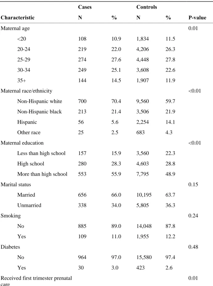
Descriptive statistics suggest that, on average, mothers of hypospadias cases tend to be
slightly older, more likely to be non-Hispanic white, lower parity, and have a higher socioeconomic
Table 2.1: Descriptive statistics for hypospadias cases and controls
Cases Controls
Characteristic N % N % P-value
Maternal age 0.01
<20 108 10.9 1,834 11.5
20-24 219 22.0 4,206 26.3
25-29 274 27.6 4,448 27.8
30-34 249 25.1 3,608 22.6
35+ 144 14.5 1,907 11.9
Maternal race/ethnicity <0.01
Non-Hispanic white 700 70.4 9,560 59.7
Non-Hispanic black 213 21.4 3,506 21.9
Hispanic 56 5.6 2,254 14.1
Other race 25 2.5 683 4.3
Maternal education <0.01
Less than high school 157 15.9 3,560 22.3
High school 280 28.3 4,603 28.8
More than high school 553 55.9 7,795 48.9
Marital status 0.15
Married 656 66.0 10,195 63.7
Unmarried 338 34.0 5,805 36.3
Smoking 0.24
No 885 89.0 14,048 87.8
Yes 109 11.0 1,955 12.2
Diabetes 0.48
No 964 97.0 15,580 97.4
Yes 30 3.0 423 2.6
Received first trimester prenatal care
No 133 13.4 2,627 16.4
Yes 861 86.6 13,376 83.6
Previous live births <0.01
No 490 49.3 6,674 41.7
Yes 504 50.7 9,329 58.3
Local Moran’s I statistics for hypospadias cases and controls show significant high-high clustering in the eastern central portion of North Carolina (Figure 2.1, Panels A and B). SaTScan
analyses (not shown) confirmed that the Census tract with 7 high-high cases also contained the center
of the only statistically significant primary cluster (p-value 0.003), with 18 observed hypospadias
cases falling within a 10.3 km radius where only 3.4 cases would have been expected. This Census
tract is located in Johnston County. From a compositional standpoint, Johnston County has a very
rapidly growing population, and a greater proportion of its population is white (80.1% vs. 71.9%
statewide) and Hispanic (13.1% vs 8.7% statewide. From a contextual standpoint, Johnston County
has historically been farmed.
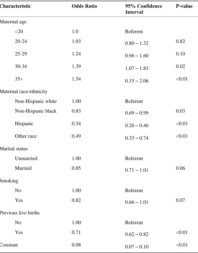
Of the eight compositional variables included in the backward stepwise logistic regression
model, five were retained (Table 2.2). Consistent with descriptive statistics, increased maternal age
and non-Hispanic white race/ethnicity were associated with increased risk. Being married and at
higher parity were associated with reduced risk. Smoking was retained in the model, with smokers at
a decreased risk, but this variable was not statistically significant. Diabetes and SES (as measured by
maternal education and month prenatal care began) were not associated with hypospadias risk in the
Table 2.2: Compositional risk factors retained by backward stepwise logistic regression model for hypospadias in North Carolina, 2003 – 2005.
Characteristic Odds Ratio 95% Confidence
Interval
P-value
Maternal age
<20 1.0 Referent
20-24 1.03 0.80 – 1.32 0.82
25-29 1.24 0.96 – 1.60 0.10
30-34 1.39 1.07 – 1.83 0.02
35+ 1.54 0.15 – 2.06 <0.01
Maternal race/ethnicity
Non-Hispanic white 1.00 Referent
Non-Hispanic black 0.83 0.69 – 0.99 0.03
Hispanic 0.34 0.26 – 0.46 <0.01
Other race 0.49 0.33 – 0.74 <0.01
Marital status
Unmarried 1.00 Referent
Married 0.85 0.71 – 1.01 0.06
Smoking
No 1.00 Referent
Yes 0.82 0.66 – 1.01 0.07
Previous live births
No 1.00 Referent
Yes 0.71 0.62 – 0.82 <0.01
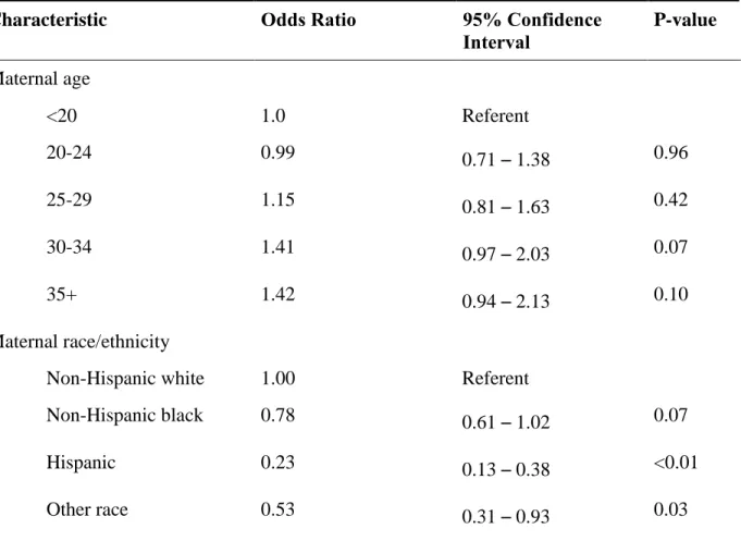
When contextual variables were incorporated into the compositional model, the natural
logarithm of the percent crop cover per block group was found to be significantly associated with
hypospadias risk (Table 2.3). Other land use variables (developed land, pasture, and forest) were not
significant and were excluded from the final model. The number of male births per block group was
not statistically significant, but was retained in the final model to control for background population
size. Overall model fit improved in the contextual model, with the Akaike information criterion
(AIC) reducing from 7469.1 with the compositional model to 3828.3 with the contextual model. The
local Moran’s I of the standardized residuals from the final model shows somewhat less spatial clustering of unexplained risk in the eastern central portion of the state, although the primary cluster
remains in Johnston County (Figure 2.1, Panel D).
Table 2.3: Results of logistic regression model including compositional and contextual risk factors for hypospadias in North Carolina, 2003 – 2005.
Characteristic Odds Ratio 95% Confidence
Interval
P-value
Maternal age
<20 1.0 Referent
20-24 0.99 0.71 – 1.38 0.96
25-29 1.15 0.81 – 1.63 0.42
30-34 1.41 0.97 – 2.03 0.07
35+ 1.42 0.94 – 2.13 0.10
Maternal race/ethnicity
Non-Hispanic white 1.00 Referent
Non-Hispanic black 0.78 0.61 – 1.02 0.07
Hispanic 0.23 0.13 – 0.38 <0.01
Marital status
Unmarried 1.00 Referent
Married 0.84 0.66 – 1.07 0.15
Smoking
No 1.00 Referent
Yes 0.77 0.58 – 1.02 0.07
Previous live births
No 1.00 Referent
Yes 0.84 0.66 – 0.98 0.03
Natural log of % of block group in crops
1.05 1.01 – 1.10 0.02
Number of male births per block group
1.00 0.99 – 1.00 0.29
18
Figure 2.1: Local spatial autocorrelation of hypospadias cases and model residuals in North Carolina 2003-2005. Panel A shows local spatial autocorrelation of hypospadias cases by Census tracts statewide. Panel B – D show spatial
Discussion
Moran’s I analysis identified significant local spatial autocorrelation of hypospadias risk in North Carolina between 2003 and 2005. Backward stepwise logistic regression identified several
important population-level factors contributing to hypospadias risk. However, local spatial
autocorrelation remained even when controlling for these effects, which suggested that contextual, or
environmental, factors might be playing a role in the distribution of hypospadias in this area.
Spatial autocorrelation of residuals was concentrated in eastern central North Carolina, which
is known for its agricultural production, particularly hog farming, flue-cured tobacco, soybeans, and
sweet potatoes (45). In fact, logistic regression indicated that the natural logarithm of percent of land
cover in crops per block group was positively associated with hypospadias risk. Further, when crop
cover and the number of live births per block group were included in the model, spatial clustering of
the standardized residuals was somewhat diminished. This suggests that exposure to agriculture may
be associated with hypospadias risk and lends indirect support to the somewhat conflicting evidence
that exposure to pesticides may play a role.
This study only has access to information about maternal address at birth, not during the
critical window of development. It also does not have information about place of work, which means
that if mothers moved during their pregnancy, or if they spent significant amounts of time outside the
home, we may not be accurately capturing contextual effects. Yet a study of exposure to air
pollution using New York data found that only 16.5% of mothers moved during pregnancy, and most
moved within such short distances that exposure assignments did not change substantially (46).
such misclassification is likely to be non-differential, which would tend to bias the results toward the
null (47).
This study illustrates the potential contribution of mapping the spatial distribution of disease
to generating hypotheses about disease etiology, and to investigating the relative contribution of
contextual and compositional effects. The associations found with hypospadias in this analysis
should not be interpreted as implying causality, and further research is needed to evaluate these
findings. Future work will investigate the mechanism by which exposure to agriculture may be
contributing to hypospadias risk in North Carolina. This ultimately might help inform policy
CHAPTER 3
USING GEOGRAPHIC CLUSTERING TO GENERATE HYPOTHESES ABOUT HYPOSPADIAS
The previous chapter uses geographic clustering methods to explore the geographic distribution of hypospadias and generate hypotheses about contextual factors that might play a
role in hypospadias risk. As discussed, local Moran’s I identified significant spatial
autocorrelation of hypospadias in eastern central North Carolina. Backwards stepwise logistic regression found a number of compositional characteristics, including maternal race, maternal age, and parity that were associated with hypospadias. These factors could not, however, fully explain the spatial autocorrelation observed in eastern central North Carolina. This led to
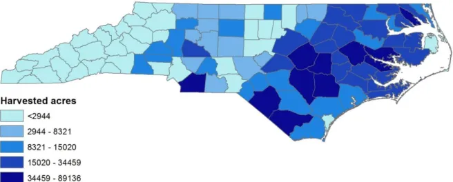
Figure 3.1: Distribution of soybean production in North Carolina, 2007
CHAPTER 4
COMPARISON OF EXPOSURE METRICS FOR ESTIMATING MATERNAL EXPOSURE TO ATRAZINE
Introduction
Hypospadias is one of the most common birth defects in the United States, affecting approximately 1 in 125 live male births. It is characterized by a urethral opening located on the ventral side of the penis, and is hypothesized to have a multifactorial etiology, where genetic susceptibility may combine with endocrine disrupting chemicals to lead to an increased risk (4).
One endocrine disrupting chemical that has been examined for a possible association with hypospadias is atrazine, which is one of the most widely used herbicides in the United States. It has been studied for potential teratogenic effects because it may disrupt normal functioning of the endocrine system and because it remains in the environment for long periods of time (35). Atrazine is commonly found in groundwater and surface water in the United States, (49) exposing humans via contaminated drinking water (35).
Chevrier et al, suggested a weak association between atrazine or atrazine metabolites and male genital anomalies, but the finding was not statistically significant, possibly due to the small sample size (54).
Because of the expense associated with both urinalysis and prospective study design, and to ensure sufficient sample size, most other studies examining a possible relationship between atrazine and adverse birth outcomes have relied on a retrospective ecological exposure
assessment. Several of these studies have assigned mothers an atrazine concentration based on monitoring samples from their public water utility (55-58). Other studies estimated exposure by assigning mothers the estimated amount of atrazine applied to their county of residence (43, 59, 60).
Chevrier et al found atrazine metabolites in urine more frequently amongst women living in rural areas and amongst women living in municipalities with the highest level of atrazine contaminated tap water (54). It is unclear, however, whether either of the commonly used ecological approaches to atrazine exposure assessment (water utility monitoring data or county-level estimates) would accurately estimate atrazine or its metabolites in urine, or how well they would correspond to one another. While this study does not have access to urinalysis data, it seeks to compare the two most common exposure assessment techniques, along with a third, novel, technique in order to consider the effects of different exposure assessment metrics on hypospadias risk estimates.
Methods
This study used data from the North Carolina Birth Defects Monitoring Program (NCBDMP), which collects data on infants born with congenital abnormalities in North
Carolina. Trained field staff collect birth defect data from hospital medical records. NCBDMP combines these data with other administrative data from hospital discharge data, vital records, and Medicaid claims, including geocoded maternal residential address at birth.
Hypospadias is classified by severity, based on the location of the urethral opening. First degree cases are the mildest and most common, with severity increasing in second and third degree cases (4). Because any potential role played by endocrine disrupting chemicals may be subtle, we included all levels of severity in this study. Cases therefore included all successfully geocoded first-, second-, and third-degree hypospadias cases (n=1,172) born in North Carolina between 2003 and 2005. Controls (n=17,635) consisted of a 10% random sample of all male births in North Carolina during the same time period.
Exposure assessment metrics:
Maternal exposure was estimated using three different methods in order to compare two exposure estimation techniques used by other studies of atrazine and birth defects, as well as a third exposure estimation technique. All three methods used residential address at birth and year of conception, estimated by subtracting estimated gestational age from date of birth. Because we did not have access to water quality monitoring data beyond public water supplies, women using private wells were excluded from this analysis.
The first exposure estimation technique, referred to hereafter as the county metric, used
the “Annual county atrazine use estimates for agriculture, 1992-2007” dataset from the US
Geological Survey (USGS) (61). This dataset was created by combining proprietary data from the DRMKynetic AgroTrak database on the total mass of atrazine applied annually to crops with data on harvested crop acreage from the US Department of Agriculture Censuses of Agriculture and the National Agriculture Statistics Service.
We assigned mothers to a county by overlaying maternal residential address with polygons of North Carolina counties using ArcGIS version 10. Mothers were assigned an exposure based on the estimated number of tons of atrazine per square mile applied to their county of residence during their estimated year of conception.
The county metric was then divided into four categories based on the exposure
distribution of the controls. Because we had non-normally distributed data, we set cut points to maximize the interval between groups. The first category (referent) was equal to the first decile of exposure in the controls; the second category was equal to the second through fifth deciles; the third category was equal to the sixth through eighth deciles; and the fourth category was equal to the ninth and tenth deciles.
Exposure estimation using US Environmental Protection Agency monitoring data:
The second exposure estimation technique, referred to hereafter as the monitoring metric,
used data from the US Environmental Protection Agency’s (EPA) Six-Year Review Contaminant
Samples collected with values less than or equal to EPA’s maximum residue limit (MRL) for
atrazine were recorded as the MRL, or 0.1 micrograms per liter (µg/L). Samples exceeding the MRL were recorded as the actual recorded concentration.
We assigned mothers to a water utility by overlaying maternal residential address with public water system service area polygons from the North Carolina Center for Geographic Information and Analysis (63). Mothers were assigned an atrazine concentration based on the mean value of all available monitoring samples for their water supply for the calendar year of their conception.
Because of the high number of samples recorded at or below the MRL, the monitoring metric was categorized as a binary variable, with mothers at or below the MRL categorized as unexposed, and mothers above the MRL categorized as exposed.
Exposure estimation using US Geological Survey atrazine models:
The third method, referred to hereafter as the watershed modeling metric, combined estimates from USGS models estimating atrazine concentrations in streams and in groundwater. For streams, we used the estimated annual mean atrazine concentration predicted by the
For groundwater estimates, we used site-variable model predictions from the “Regression
Models for Estimating Concentrations of Atrazine plus Deethylatrazine in Shallow Groundwater
in Agricultural Areas of the United States.” This model is derived from a residence-time
indicator, atrazine use intensities, artificial drainage, depth to the seasonally high water-table, organic matter content of the uppermost soil layer, permeability of the least permeable soil layer, rate of recharge, and well depth. (38).
We then used geographic coordinates for surface and groundwater intakes from the North Carolina Division of Environmental Health to link atrazine concentrations to public water
utilities (64). For surface water intakes, we used WARP estimates from the nearest stream reach to assign an annual mean atrazine concentration to the intake. For groundwater intakes, we used gridded atrazine predictions from the USGS groundwater model and bilinear interpolation to estimate atrazine concentrations based on the grid cell where the intake was located and the adjacent grid cells. Each public water utility was then assigned an atrazine concentration equal to the mean of the predicted atrazine concentrations for all of the intakes for that utility. Mothers were assigned an atrazine concentration using public water supply polygons as outlined for the monitoring metric.
Comparison of exposure metrics:
The three exposure metrics were compared both as continuous and as categorical
variables to consider the differences between each exposure assessment metric. The categorized county and watershed modeling metrics and the binary EPA metric were first mapped to
visualize the geographic distribution and degree of missingness for the three metrics. Continuous metrics were then compared using Pearson correlation coefficients.
Categorized and binary metrics were compared using weighted kappa statistics. The kappa statistic measure of agreement is 0 when the amount of agreement is what would be expected due to chance and 1 when there is perfect agreement. The weighted kappa statistic is used for comparing ranked categories. It assigns categorizations that agree completely a weight of 1; categorizations that are near one another a weight closer to 1; and categorizations further apart a weight closer to 0. For example, if a mother was placed in the third category by the county metric and in the fourth category by the watershed modeling metric, she would receive a weight of 0.667, but if she was placed in the second category by the county metric and in the fourth category by the watershed modeling metric, she would receive a weight of 0.333.
We also calculated risk estimates for hypospadias using both the continuous and
categorized metrics using logistic regression. We then compared how different exposure metrics influenced risk estimates for hypospadias. The purpose of these analyses was not to estimate the risk associated with exposure to atrazine, per se, but rather to examine if and how the exposure assessment metrics performed differently in epidemiologic models. We performed all
Results
Figure 4.1 illustrates the geographic distribution of each of the three metrics. The county metric has the most comprehensive geographic distribution. While the monitoring and
watershed modeling metric both display a large degree of missingness, there is at least some geographic overlap between the watershed modeling metric and the county metric and between the watershed modeling metric and the monitoring metric. The water utilities classified as highly exposed generally seem to fall in counties classified in the third and fourth categories of
Table 4.1 presents the distribution of each of the continuous exposure metrics. The mean and median values for the county metric are 12.9 and 6.8 lbs/mi2, respectively (interquartile range = 2.7-14.8). The mean and median values for the watershed modeling metric are 0.05 and 0.04 µg/L, respectively (interquartile range (0.03-0.05). The distribution for the monitoring metric is highly skewed, however, with the minimum, mean, median, and 75th percentile values all equal to 0.1.
Table 4.1: Distribution of continuous exposure metrics
Exposure metric Mean Median Interquartile range Min, Max values
County metric (in lbs/mi2)
12.9 6.8 2.7, 14.8 0.04, 287.0
Monitoring metric (in
µg/L)
0.1 0.1 0.1, 0.1 0.1, 1.2
Watershed modeling metric (in µg/L)
0.05 0.04 0.03, 0.05 0.01, 0.5
Table 4.2 presents Pearson correlation coefficients between the three continuous exposure metrics. Correlation coefficients range from 0.23 to 0.62, with the county and
monitoring metrics least correlated with each other and the monitoring and watershed modeling metrics most correlated with one another.
Table 4.2: Pearson correlation coefficients between continuous exposure metrics assigned to women who delivered a baby in North Carolina (N)
Exposure metrics compared N Pearson Correlation
County and monitoring 6,933 0.23
Comparisons between categorized exposure assessment metrics are presented in Tables 4.3 - 4.5. Weighted kappa values are all significantly different from 0. Agreement is lower when comparing the monitoring metric to either the watershed modeling metric or county metrics, with weighted kappa values of 0.01 and agreement at between 47% and 56% (Tables 4.3-4.4). Agreement is slightly higher when comparing the watershed modeling and county metrics, with a weighted kappa value of 0.29, and 77% agreement (Table 4.5).
Table 4.3: Comparison of categorized watershed modeling metric and binary monitoring metric
Watershed modeling category
1 2 3 4 Total
Monitoring (unexposed) 462 1163 878 248 2751
Monitoring (exposed) 0 10 102 66 178
Total 462 1173 980 314 2929
Weighted kappa = 0.01 (p <0.01). Percent agreement = 55.65%
Table 4.4: Comparison of categorized county metric and binary monitoring metric County category
1 2 3 4 Total
Monitoring (unexposed) 1236 2146 1591 1781 6754
Monitoring (exposed) 0 72 87 20 179
Total 1172 3089 1713 959 6933
Weighted kappa = 0.01 (p< 0.01). Percent agreement = 47.95%
Table 4.5: Comparison of categorized watershed modeling and county metrics
Watershed modeling category
County category 1 198 200 0 0 598
County category 2 215 520 1013 23 1771
County category 3 54 690 1332 260 2336
County category 4 65 411 798 333 1307
Total 732 1821 3143 616 6312
Weighted kappa = 0.29 (p < 0.01). Percent agreement = 77.0%
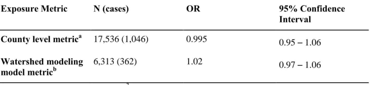
Table 4.6 compares crude risk estimates for hypospadias for the county and watershed modeling exposure metrics on a continuous scale. Crude risk estimates could not be computed for the monitoring metric due to the lack of variability as described in Table 4.1. The odds ratio from the county level metric is 0.97, and the odds ratio from the watershed modeling metric is 2.29. The odds ratio greater than one from the watershed modeling metric suggests a positive relationship, while the odds ratio near one for the county level metric suggests no association; however, neither of the estimates is statistically significant.
Table 4.6: Comparison of crude risk estimates from continuous scale exposure assessment metrics.
Exposure Metric N (cases) OR 95% Confidence
Interval
County level metrica 17,536 (1,046) 0.995 0.95 – 1.06 Watershed modeling
model metricb
6,313 (362) 1.02 0.97 – 1.06
a
increment of change = 12.1 lb/mi2 IQR
b
increment of chang e= 0.02 µg/L IQR
a slightly elevated risk in the highest categories of exposure, with odds ratios of 1.14 and 1.23 respectively, but again, neither of the estimates is statistically significant.
Table 4.7: Comparison of risk estimates from categorized exposure assessment metrics Exposure Metric Estimated Atrazine
Level
N (cases) Odds Ratio
95% Confidence Interval
County metric Category 1 (<1.6 lbs/mi2)
1,940 (102) 1.0 Referent
Category 2 (1.6 – 5.2 lbs/mi2)
4,964 (291) 1.12 0.89 – 1.41
Category 3
(5.2 – 14.1 lbs/mi2)
5,362 (340) 1.22 0.97 – 1.53
Category 4 (>14.1 lbs/mi2)
5,270 (313) 1.14 0.90 – 1.43
Watershed modeling metric
Category 1
(0.006 – 0.017 µg/L)
732 (43) 1.0 Referent
Category 2
(0.017 – 0.033 µg/L)
1,821 (92) 0.85 0.59 – 1.24
Category 3
(0.033 – 0.074 µg/L)
3,143 (183) 0.99 0.70 – 1.40
Category 4
(0.076 – 0.50 µg/L)
606 (44) 1.23 0.80 – 1.90
Discussion
A number of studies have attempted to estimate prenatal exposure to atrazine via drinking water in order to evaluate possible teratogenic effects of atrazine (43, 55-60). These studies have generally used residential address to either assign mothers to counties or to drinking water
This study considers how different exposure metrics might influence estimated exposure
to atrazine by comparing two metrics used by other studies – the county metric and the
monitoring metric – as well as a third metric which uses USGS model outputs to estimate
atrazine in drinking water. The three metrics are compared using maps, Pearson correlation coefficients and kappa statistics. The county metric and the watershed modeling metric are also compared using and unadjusted odds ratios of hypospadias risk.
The maps and Pearson correlation coefficients found the watershed modeling metric to be more similar to the county and monitoring metrics, with the monitoring metric to be less similar to the county metric. The kappa statistic found the watershed modeling and county exposure metrics to be more similar than either the monitoring metric and county metric or the monitoring metric and watershed modeling metric. Because the watershed modeling metric includes
atrazine use at the county level, and estimates exposure for water utilities, it makes sense that the watershed modeling metric has more in common with the county metric and the monitoring metric than county metric and monitoring metric have in common with one another.
hypospadias. However, they do illustrate the differences in odds ratios produced by different exposure metrics.
Although it is impossible to know whether any of the exposure metrics explored in this
study approximate the “true” level of atrazine exposure, there are trade-offs associated with each
of the exposure metrics. Because the vast majority of monitoring samples at public water utilities in North Carolina during the study period were at or below the MRL, and because North Carolina does not report data about atrazine concentrations at or below the MRL, the monitoring metric provided very little variation in estimated exposure, which prevented us from estimating odds ratios for hypospadias using this metric. Some states do report values for concentrations below the MRL, so it is possible that these data might provide more useful estimates of exposure in other states. For North Carolina, however, a lack of data prevents us from considering effects that might occur below the 0.1 µg/L threshold set by EPA.
The county metric provides exposure estimates to a much larger proportion of the study population and provides greater variation in estimated exposure. It may also be more prone to the ecological fallacy, however, because average pesticide use at the county level may not be an accurate indicator of individual exposure.
The watershed modeling metric attempts to address some of these shortcomings by providing a wider range of estimated exposure, and by incorporating the way that surface water flows through a watershed or groundwater moves through soils. On the other hand, the USGS models are not designed to address residence time in reservoirs or lakes, so therefore may not be accurately estimating atrazine concentrations in public water utilities.
only one of the metrics is a good surrogate for estimating atrazine exposure, although it is
impossible to confirm which one is the “good” one without knowledge of the actual amount of
atrazine to which women were exposed. On the other hand, it could also indicate that none of the metrics is a good surrogate for estimating atrazine exposure, but simply that each is measuring something different.
A limitation of all of the metrics explored in this study is the use of a calendar year cut-off to assign exposure. Because the exposure metrics relied on annual mean atrazine estimates, the exposure estimate for a baby conceived in December would be based on mean estimates for the prior year, while the exposure estimate for a baby conceived in January would be based on mean estimates for the coming year. This may lead to exposure misclassification, particularly for winter births.
A further limitation of all of the metrics is the lack of information about maternal water consumption. If hypospadias risk increases when genetic susceptibility combines with endocrine disrupting chemicals exceeding some threshold, it would be important to know both the
concentrations the chemicals of interest in drinking water, as well as the amount of drinking water consumed in estimating a threshold.
On the other hand, given the expense associated with prospective studies of birth outcomes including urinalysis for a given exposure, ecological exposure estimation techniques may be useful for identifying potential teratogens for further study. Difference in the magnitude and direction of odds ratios the importance of exposure measurement in estimating disease risk. Further research is needed to better understand the potential role played by atrazine in
CHAPTER 5
SELECTING AN EXPOSURE METRIC TO EXAMINE A RELATIONSHIP BETWEEN ATRAZINE AND HYPOSPADIAS
The previous chapter compared three different metrics for estimating maternal exposure to atrazine via drinking water: the county metric, which uses the amount of atrazine applied to a
mother’s county of residence; the monitoring metric, which uses water quality samples collected
for compliance monitoring; and the watershed modeling metric, which uses output from USGS surface water and groundwater models to estimate atrazine concentrations in public water utilities. Although there are limitations associated with each of these metrics, the county metric does not provide an estimate of concentrations in drinking water, and may be more subject to the ecological fallacy than the other metrics. Further, the monitoring metric does not provide
information about atrazine concentrations below EPA’s MRL. The watershed modeling metric
overcomes the shortcomings associated with the other two metrics because it is able to estimate concentrations in individual water supplies, and at a full range of exposures. The next chapter will therefore use the watershed modeling metric to examine a possible association between atrazine and hypospadias risk.
The previous chapters used data from the North Carolina Birth Defect Monitoring Program (NCBDMP) in order to explore the etiology of hypospadias and to compare different exposure estimation techniques. Although NCBDMP data contains information about
residential address throughout pregnancy. In order to consider a possible association between atrazine and hypospadias within a disease ecology framework, the next chapter will use data from the National Birth Defects Prevention Study (NBDPS), which includes behavioral
CHAPTER 6
HYPOSPADIAS AND MATERNAL EXPOSURE TO ATRAZINE
Introduction
Hypospadias is a relatively common birth defect of the male urinary tract, affecting between 4 and 6 out of every 1,000 male births. It occurs as a result of abnormal urethral closure during gestational weeks 8-14, and manifests with a urethral opening on the underside of the penis (1). It has a significant public health impact, as surgical repair is often needed to allow for normal urinary and sexual function, and even after correction, hypospadias may result in
psychosocial and sexual problems later in life (3).
42
There is experimental evidence to support a link between atrazine and genitourinary malformations in both rats (50) and amphibians (33, 51-53). The evidence to document a specific link between hypospadias and atrazine in humans is somewhat equivocal, however.
Winchester et al found an elevated prevalence of “other urogenital anomalies,” but not of
“malformed genitalia” among infants conceived during months of the highest concentrations of
atrazine and other chemicals measured by the US Geological Survey’s National Water Quality
Assessment Program (23). Chevrier et al examined urinary biomarkers of atrazine and general male genital anomalies. They found a non-significant increase in male genital anomalies
amongst mothers with quantifiable atrazine or atrazine metabolites in urine, but their sample size was small (5 cases exposed and 18 case unexposed) (54). To our knowledge, only two studies have looked specifically at atrazine and hypospadias in humans, with conflicting results. The first study, by Meyer et al, 2006, assigned maternal exposure to several agricultural pesticides (including atrazine) by estimating the amount of pesticides applied within a 500 meter buffer of
the mother’s home. They did not find evidence of an association between hypospadias and
atrazine (36). The second study, by Agopian et al, 2013, assigned atrazine levels to mothers based on their county of residence at birth. They found some evidence of an increased risk of hypospadias for mothers in the 25th-75th percentiles of exposure and for the 75th-90th percentiles of exposure, but suggested that further research was needed to confirm the mechanism for an association between hypospadias and county level atrazine use (43).
combine with other maternal demographic and behavioral characteristics to influence hypospadias risk. A number of maternal characteristics have previously been linked to
hypospadias risk. From a demographic standpoint, risk increases with increasing maternal age (10, 14) and is higher amongst non-Hispanic white mothers (10, 39). There is conflicting evidence about an association with maternal education (12, 39, 66), but evidence of an inverse association with maternal parity (12, 67, 68) and of a positive association with plurality (7, 12, 69). Amongst behavioral characteristics, maternal diet may influence risk, with higher dietary intake of choline, methionine, and vitamin B12 associated with lower risk (11). Use of fertility medications and procedures, on the other hand, seems to increase risk (17, 69, 70).
In this study, we seek to build on existing research examining the potential relationship between atrazine and hypospadias by incorporating information about maternal water
consumption, as well as other known demographic and behavioral risk factors. We use a novel technique to estimate maternal exposure to atrazine in drinking water, and take advantage of unique data that includes information about behavioral covariates and maternal residential address throughout pregnancy. This allows us to investigate the role of atrazine in conjunction with other factors that may contribute to the multi-factorial etiology of hypospadias.
Methods
Data from this study comes from the National Birth Defects Prevention Study (NBDPS), which is a population-based case-control study conducted in ten states with the Centers for Disease Control and Prevention. NBDPS identifies second- and third-degree hypospadias cases, which are considered moderate to severe (1), from birth defect surveillance registries and
include first-degree, or mild, hypospadias cases due to variable medical documentation. NBDPS also collects data on a wide number of covariates via computer-assisted telephone interview. Covariates include information about water consumption, maternal address throughout pregnancy, and a number of known risk factors for hypospadias, including maternal age,
maternal race/ethnicity, parity, plurality, maternal choline intake, and use of fertility medications (71).
The study included interviewed hypospadias cases (n= 343) and male controls (n=1,422) from North Carolina, Iowa, Arkansas, and Texas with estimated due dates between 1998 and 2005. These states were selected from the NBDPS study sites because atrazine concentrations in streams were predicted to be higher than in other study sites (72). These years were selected because they were the years for which data were collected about water consumption.
Mothers using a public water supply were assigned a water utility for each reported residential address by the University of Iowa Center for Health Effects of Environmental
Contamination (CHEEC), using public water supply service area polygons where available, and Census place names and borders where service area polygons were unavailable.
We estimated atrazine concentrations using two US Geological Survey (USGS) models. For water supplies using surface water, we used estimated annual mean atrazine concentrations in streams predicted by the Watershed Regressions for Pesticides (WARP) model. WARP uses
estimated watershed-level atrazine use, the percentage of the watershed’s agricultural land with a
water supplies using groundwater, we used site-variable model predictions from the “Regression
Models for Estimating Concentrations of Atrazine plus Deethylatrazine in Shallow Groundwater
in Agricultural Areas of the United States.” This model uses groundwater residence time,
atrazine use intensity, artificial drainage practices, depth to the seasonally high water-table, content of the uppermost soil content, soil permeability, groundwater recharge rates, and well depth to provide gridded estimates of atrazine concentrations in shallow groundwater (38).
We assigned atrazine concentrations to public water supplies based on the type and location of the water intakes for each utility. Geographic coordinates of surface and groundwater intakes for public water utilities were available for Iowa, Texas, and North Carolina (64, 73-75). For Arkansas, we used Google Earth to geocode water intakes using descriptions of intake locations available from the Arkansas Department of Health (76).
47
We based our exposure assessment on maternal residential addresses during gestational weeks 6-16. This window encompass the critical weeks for urethral development during gestational weeks 8-14 (42). Mothers using public water were assigned an atrazine exposure based on the estimated atrazine concentration in the public water utility assignments from CHEEC. Mothers using well water were assigned an atrazine value based on bilinear interpolation of gridded atrazine predictions from the USGS groundwater model. This assignment was conducted using ArcGIS version 10. Mothers with more than one residential address during the critical exposure period were assigned a weighted value based on the atrazine concentration and the number of weeks at each address. We excluded mothers without a full residential history, mothers using public water who were not successfully matched to a public water utility, and mothers using a utility that was not successfully assigned an atrazine
concentration by one of the two USGS models. This reduced our sample size to 123 cases and 415 controls. We conducted a sensitivity analysis to help characterize any selection bias that might be introduced by this loss of sample size.
We then estimated the daily amount of atrazine consumed via drinking water by a mother
by multiplying the estimated atrazine concentration in a mother’s drinking water by the
self-reported number of glasses of water drunk daily by the mother. The self-self-reported number of glasses consumed ranged from 0 to 24 glasses of water daily. Because it is unlikely that pregnant women are consuming no water, we converted the women who reported drinking 0 glasses to missing prior to multiplying by estimated atrazine concentration.
We then built unadjusted and adjusted logistic regression models for two predictors of interest:
estimated concentration of atrazine in a mother’s drinking water supply; and for estimated daily
maternal atrazine consumption. We estimated crude and adjusted odds ratios for hypospadias for both predictors. Covariates used for adjustment were selected based on existing literature, and included private well use, state of residence, maternal age, maternal race/ethnicity, plurality, parity, maternal education, choline use, and use of artificial reproductive technology as possible confounders. Analyses were performed using Stata version 13.1.
Results
We present the distributions of socioeconomic, demographic, and behavioral
characteristics for mothers of hypospadias cases (n = 123) and male controls (n = 415) in Table 6.1. Significant differences in distribution between cases and controls were observed for state of residence, maternal race or ethnicity, maternal education, previous pregnancies, plurality, and use of fertility medications or procedures. While controls were fairly evenly distributed amongst the four states, 79.6% of cases lived in Arkansas and North Carolina. Mothers of cases were more likely to be non-Hispanic white, more highly educated, and to have used fertility
Table 6.1: Characteristics of NBDPS hypospadias cases and controls with estimated atrazine exposure, 1998-2005
Cases Controls
Characteristic N % N % P-value
State of residence <0.01
Arkansas 49 39.8 85 20.5
Iowa 17 13.8 103 24.8
Texas 8 6.5 101 24.3
North Carolina 49 39.8 126 30.4
Private well use 0.72
No 85 70.3 292 71.9
Yes 36 29.7 114 28.1
Reported water consumption 0.09
0 glasses 3 2.4 22 5.3
1-4 glasses 77 62.6 217 52.3
5 or more glasses 43 35.0 176 42.4
Maternal age 0.23
<20 10 8.1 43 10.4
20-24 27 22.0 89 21.5
25-29 25 20.3 118 28.4
30-34 42 34.2 105 25.3
≥35 19 15.5 60 14.5
Maternal race/ethnicity <0.01
Non-Hispanic white 94 76.4 242 58.3
Non-Hispanic black 16 13.0 32 7.7
Hispanic 8 6.5 106 25.5
Other 5 4.1 35 8.4
Maternal education <0.01
High school 30 24.4 111 26.8
>High school 88 71.5 218 52.5
Previous pregnancies <0.01
No 55 44.7 122 29.4
Yes 68 55.3 293 70.6
Plurality 0.01
No 114 92.7 405 97.6
Yes 9 7.3 10 2.4
Maternal choline intake* 0.15
<187.4 mg 27 22.0 72 17.4
187.4 – 249.6 mg 30 24.4 85 20.5
249.7 – 336.3 mg 34 27.6 104 25.1
>336.4 mg 32 26.0 154 37.1
Fertility medications or procedures 0.02
No 111 90.2 393 95.6
Yes 12 9.8 18 4.4
*Categories for maternal choline intake from Carmichael et al (11)
We present raw distributions for estimated concentrations of atrazine for a mother’s
Table 6.2: Distribution of estimated atrazine in water supply and estimated atrazine consumption
Cases Controls
Mean Median IQR Min,
Max
Mean Median IQR Min, Max
Estimated atrazine in water supply (µg/L)
0.091 0.018 0.001 –
0.04
0.0001, 2.0
0.17 0.019 0.002 –
0.051 0.0001, 4.0 Estimated atrazine consumption (µg/L)
0.491 0.066 0.004 –
0.16
0.0002, 15.8
0.61 0.073 0.010 –
0.274
0.0003, 19.7
We present crude and adjusted odds ratios for hypospadias for the estimated
concentration of atrazine in a mother’s drinking supply and for a mother’s estimated daily