Scientific Computing with MATLAB - Free Computer, Programming, Mathematics, Technical Books, Lecture Notes and Tutorials

(1)

Scientific Computing

with

MATLAB

Paul Gribble

Fall, 2015

(2)

About the author

Paul Gribble is a Professor at theUniversity of Western Ontario1_{in London,}

On-tario Canada. He has a joint appointment in theDepartment of Psychology2

and theDepartment of Physiology & Pharmacology3_{in the}_{Schulich School of}

Medicine & Dentistry4_{. He is a core member of the}_{Brain and Mind Institute}5

and a core member of theGraduate Program in Neuroscience6_{. He received his}

PhD fromMcGill University7_{in 1999. His lab webpage can be found here:}

http://www.gribblelab.org

This document

This document was typeset using LA_{TEX version 3.14159265-2.6-1.40.16 (TeX}

Live 2015). These notes in their entirety, including the LA_{TEX source, are}

avail-able onGitHub8_here:

https://github.com/paulgribble/SciComp

License

This work is licensed under aCreative Commons Attribution 4.0 International License9_{. The full text of the license can be viewed here:}

(3)

iii LINKS

Links

1_{http://www.uwo.ca}

2_{http://psychology.uwo.ca}

3_{http://www.schulich.uwo.ca/physpharm/}

4_{http://www.schulich.uwo.ca}

5_{http://www.uwo.ca/bmi}

6_{http://www.schulich.uwo.ca/neuroscience/}

7_{http://www.mcgill.ca}

8_{https://github.com}

(4)

(5)

Preface

These are the course notes associated with my graduate-level course called Sci-entific Computing (Psychology 9040a), given in the Department of Psychol-ogy10_{at the}_{University of Western Ontario}11_{. The goal of the course is to provide}

you with skills in scientific computing: tools and techniques that you can use in your own scientific research. We will focus on learning to think about experi-ments and data in a computational framework, and we will learn to implement specific algorithms using a high-level programming language (MATLAB). Learn-ing how to program will significantly enhance your ability to conduct scientific research today and in the future. Programming skills will provide you with the ability to go beyond what is available in pre-packaged analysis tools, and code your own custom data processing, analysis and visualization pipelines.

The course (and these notes) are organized around using MATLAB12 ₍

Math-Works13_{), a high-level language and interactive environment for scientific}

com-puting. MATLAB version R2015b is used throughout.

Chapters 13 and 14 on integrating ordinary differential equations and

simulat-ing dynamical systems are based on notes from a previous course that were de-veloped in collaboration with Dr. Dinant Kistemaker (VU Amsterdam).

For a much more detailed, comprehensive book on MATLAB and all of its func-tionality, I can recommend:

Mastering MATLABby Duane Hanselman & Bruce Littlefield. Pearson Eduction, Inc., publishing as Prentice Hall, Upper Saddle River, NJ, 2012. ISBN: 978-0-13-601330-3.

(6)

They have a website associated with their book here:

(7)

vii LINKS

Conventions in the notes

Web links are given in blue font and are clickable when viewing this document as a .pdf on your computer, for example:Gribble Lab14_{. Code snippets are shown}

in monospaced font within a box with a gray backround such as this:

>> disp('Hello, world!') Hello, world!

Also note that Chapter headings, sections and subsections in the Table of Con-tents are hyperlinks in this .pdf, so that if you click on them you are taken di-rectly to the appropriate page.

Comments

Do you have ideas about how to improve these notes? Please get in touch, send me an email at [email protected]

Links

10_{http://psychology.uwo.ca}

11_{http://www.uwo.ca}

12_{http://www.mathworks.com/products/matlab/}

13_{http://www.mathworks.com}

(8)

1 What is computer code? 1

1.1 High-level vs low-level languages . . . 1

1.2 Interpreted vs compiled languages . . . 5

2 Digital representation of data 9 2.1 Binary . . . 9

2.2 Hexadecimal . . . 10

2.3 Floating point values . . . 12

2.4 ASCII . . . 15

Exercises . . . 18

3 Basic data types, operators & expressions 21 3.1 Expressions . . . 21

3.2 Operators . . . 24

3.3 Variables . . . 25

3.4 Basic Data Types . . . 31

3.5 Special values . . . 38

3.6 Getting help . . . 40

3.7 Script M-files . . . 42

3.8 MATLAB path . . . 43

Exercises . . . 46

4 Complex data types 49 4.1 Arrays . . . 49

4.2 Matrices . . . 57

(9)

ix CONTENTS

4.3 Multidimensional arrays . . . 69

4.4 Cell arrays . . . 73

4.5 Structures . . . 74

Exercises . . . 80

5 Control flow 83 5.1 Loops . . . 83

5.2 Conditionals . . . 86

5.3 Switch statements . . . 88

5.4 Pause, break, continue, return . . . 88

Exercises . . . 92

6 Functions 95 6.1 Encapsulation . . . 95

6.2 Function specification . . . 97

6.3 Variable scope . . . 98

6.4 Anonymous functions . . . 100

Exercises . . . 101

7 Input & Output 107 7.1 Plain text files . . . 108

7.2 Binary files . . . 111

7.3 ASCII or binary? . . . 112

8 Debugging, profiling and speedy code 115 8.1 Debugging . . . 115

8.2 Timing and Profiling . . . 119

8.3 Speedy Code . . . 126

8.4 MATLAB Coder . . . 137

9 Parallel programming 143 9.1 What is parallel computing? . . . 143

(10)

9.3 Symmetric Multiprocessing (SMP) . . . 144

9.4 Hyperthreading . . . 146

9.5 Clusters . . . 147

9.6 Grids . . . 148

9.7 GPU Computing . . . 149

9.8 Types of Parallel problems . . . 150

9.9 MATLAB . . . 150

9.10 Shell scripts . . . 151

Exercises . . . 152

10 Graphical displays of data 157 Exercises . . . 159

11 Signals, sampling & filtering 173 11.1 Time domain representation of signals . . . 173

11.2 Frequency domain representation of signals . . . 174

11.3 Fast Fourier transform (FFT) . . . 175

11.4 Sampling . . . 175

11.5 Power spectra . . . 178

11.6 Power Spectral Density . . . 180

11.7 Decibel scale . . . 182

11.8 Spectrogram . . . 183

11.9 Filtering . . . 183

11.10 Quantization . . . 194

11.11 Sources of noise . . . 195

Exercises . . . 197

12 Optimization & gradient descent 209 12.1 Analytic Approaches . . . 212

12.2 Numerical Approaches . . . 215

12.3 Optimization in MATLAB . . . 220

(11)

xi CONTENTS

13 Integrating ODEs & simulating dynamical systems 229

13.1 What is a dynamical system? . . . 229

13.2 Why make models? . . . 231

13.3 Modelling Dynamical Systems . . . 233

13.4 Integrating Differential Equations in MATLAB . . . 236

13.5 The power of modelling and simulation . . . 239

13.6 Simulating Motion of a Two-Joint Arm . . . 239

13.7 Lorenz Attractor . . . 242

Exercises . . . 250

14 Modelling Action Potentials 255 14.1 The Neuron Model . . . 256

14.2 Passive Properties . . . 257

14.3 Sodium Channels (Na) . . . 258

14.4 Potassium Channels (K) . . . 260

14.5 Summary . . . 261

14.6 MATLAB code . . . 261

Exercises . . . 266

15 Basic statistical tests 269 15.1 Probability Distributions . . . 269

15.2 Hypothesis Tests . . . 273

15.3 Resampling techniques . . . 279

(12)

(13)

1 What is computer code?

What is a computer program? What is code? What is a computer language? A computer program is simply a series of instructions that the computer executes, one after the other. An instruction is a single command. A program is a series of instructions. Code is another way of referring to a single instruction or a series of instructions (a program).

1.1 High-level vs low-level languages

TheCPU15_{(central processing unit) chip(s) that sit on the}_motherboard16_{of your}

computer is the piece of hardware that actually executes instructions. A CPU only understands a relatively low-level language calledmachine code17_{. Often}

machine code is generated automatically by translating code written in assem-bly language18_{, which is a}_{low-level programming language}19 _{that has a}

rela-tively direcy relationship to machine code (but is more readable by a human). A utility program called anassembler20 _{is what translates assembly language}

code into machine code.

In this course we will be learning how to program in MATLAB, which is a high-level programming language21_{. The “high-level” refers to the fact that the}

lan-guage has a strong abstraction from the details of the computer (the details of the machine code). A “strong abstraction” means that one can operate using high-level instructions without having to worry about the low-level details of carrying out those instructions.

An analogy is motor skill learning. A high-level language for human action

(14)

might bedrive your car to the grocery store and buy apples. A low-level version of this might be something like: (1) walk to your car; (2) open the door; (3) start the ignition; (4) put the transmission into Drive; (5) step on the gas pedal, and so on. An even lower-level description might involve instructions like: (1) activate yourgastrocnemius muscle22_{until you feel 2 kg of pressure on the underside of}

your right foot, maintain this pressure for 2.7 seconds, then release (stepping on the gas pedal); (2) move your left and right eyeballs 27 degrees to the left (check for oncoming cars); (3) activate your pectoralis muscle on the right side of your chest and simultaneously squeeze the steering wheel with the fingers on your right hand (steer the car to the left); and so on.

For scientific programming, we would like to deal at the highest level we can, so that we can avoid worrying about the low-level details. We might for exam-ple want to plot a line in a Figure and colour it blue. We don’t want to have to program the low-level details of how each pixel on the screen is set, and how to generate each letter of the font that is used to specify the x-axis label.

As an example, here is ahello, worldprogram written in a variety of languages, just to give you a sense of things. You can see the high-level languages like MAT-LAB, Python and R are extremely readable and understandable, even though you may not know anything about these languages (yet). The C code is less readable, there are lots of details one may not know about... and the assembly language example is a bit of a nightmare, obviously too low-level for our needs here.

MATLAB

disp('hello, world')

Python

print "hello, world"

(15)

3 1.1. HIGH-LEVEL VS LOW-LEVEL LANGUAGES

cat("hello, world\n")

Javascript

document.write("hello, world");

Fortran

print *,"hello, world"

C

#include <stdio.h>

int main (int argc, char *argv[]) { printf("hello, world\n");

return 0; }

8086 Assembly language

; this example prints out "hello world!"

; by writing directly to video memory.

; in vga memory: first byte is ascii character, byte that follows is character attribute.

; if you change the second byte, you can change the color of ; the character even after it is printed.

; character attribute is 8 bit value,

; high 4 bits set background color and low 4 bits set foreground color.

; hex bin color

;

; 0 0000 black

; 1 0001 blue

; 2 0010 green

; 3 0011 cyan

(16)

; 5 0101 magenta

; 6 0110 brown

; 7 0111 light gray

; 8 1000 dark gray

; 9 1001 light blue

; a 1010 light green

; b 1011 light cyan

; c 1100 light red

; d 1101 light magenta

; e 1110 yellow

; f 1111 white

org 100h

; set video mode

mov ax, 3 ; text mode 80x25, 16 colors, 8 pages (ah=0, al=3)

int 10h ; do it!

; cancel blinking and enable all 16 colors: mov ax, 1003h

mov bx, 0 int 10h

; set segment register:

mov ax, 0b800h

mov ds, ax

; print "hello world"

; first byte is ascii code, second byte is color code.

mov [02h], 'H' mov [04h], 'e'

mov [06h], 'l' mov [08h], 'l'

mov [0ah], 'o'

mov [0ch], ',' mov [0eh], 'W'

mov [10h], 'o' mov [12h], 'r'

(17)

5 1.2. INTERPRETED VS COMPILED LANGUAGES

mov [16h], 'd'

mov [18h], '!'

; color all characters:

mov cx, 12 ; number of characters.

mov di, 03h ; start from byte after 'h'

c: mov [di], 11101100b ; light red(1100) on yellow(1110)

add di, 2 ; skip over next ascii code in vga memory. loop c

; wait for any key press: mov ah, 0

int 16h

ret

1.2 Interpreted vs compiled languages

Some languages like C and Fortran arecompiled languages23_{, meaning that we}

write code in C or Fortran, and then to run the code (to have the computer ex-ecute those instructions) we first have to translate the code into machine code, and then run the machine code. The utility function that performs this trans-lation (compitrans-lation) is called acompiler24_{. In addition to simply translating a}

high-level language into machine code, modern compilers will also perform a number of optimizations to ensure that the resulting machine code runs fast, and uses little memory. Typically we write a program in C, then compile it, and if there are no errors, we then run it. We deal with the entire program as a whole. Compiled program tend to be fast since the entire program is compiled and op-timized as a whole, into machine code, and then run on the CPU as a whole.

Other languages, like MATLAB, Python and R, are interpreted languages25_,

(18)

done using a utility called aninterpreter26_{. We don’t have to compile the whole}

program all together in order to run it. Instead we can run it one instruction at a time. Typically we do this in an interactive programming environment where we can type in a command, and observe the result, and then type a next com-mand, etc. This is known as the27_{. This is}

advan-tageous for scientific programming, where we typically spend a lot of time ex-ploring our data in an interactive way. One can of course run a program such as this in a batch mode, all at once, without the interactive REPL environment... but this doesn’t change the fact that the translation to machine code still hap-pens one line at a time, each in isolation. Interpreted languages tend to be slow, because every single command is taken in isolation, one after the other, and in real time translated into machine code which is then executed in a piecemeal fashion.

For interactive programming, when we are exploring our data, interpreted lan-guages like MATLAB, Python and R shine. They may be slow but it (typically) doesn’t matter, because what’s many orders of magnitude slower, is the firing of the neurons in our brain as we consider the output of each command and decide what to do next, how to analyse our data differently, what to plot next, etc. For batch programming (for example fMRI processing pipelines, or

electro-physiological recording signal processing, or numerical optimizations, or statis-tical bootstrapping operations), where we want to run a large set of instructions

all at once, without looking at the result of each step along the way, compiled languages really shine. They are much faster than interpreted languages, often several orders of magnitude faster. It’s not unusual for even a simple program written in C to run 100x or even 1000x faster than the same program written in MATLAB, Python or R.

A 1000x speedup may not be very important when the program runs in 5 sec-onds (versus 5 millisecsec-onds) but when a program takes 60 secsec-onds to run in MATLAB, for example, things can start to get problematic.

(19)

7 1.2. INTERPRETED VS COMPILED LANGUAGES

that so bad? Not if you only have to run it once. Now let’s imagine you have 15 subjects in your group. Now 60 seconds is 15 minutes. Now let’s say you have 4 groups. Now 15 minutes is one hour. You run your program, go have lunch, and come back an hour later and you find there was an error. You fix the error and re-run. Another hour. Even if you get it right, now imagine your supervisor asks you to re-run the analysis 5 different ways, varying some parameter of the analysis (maybe filtering the data at a different frequency, for example). Now you need 5 hours to see the result. It doesn’t take a huge amount of data to run into this sort of situation.

Now imagine if you could program this data processing pipeline in C instead, and you could achieve a 500x speedup (not unusual), now those 5 hours turn into 36 seconds (you could run your analysis twice and it would still take less time than listening to Stairway to Heaven a dozen times). All of a sudden it’s the difference between an overnight operation and a 30 second operation. That makes a big difference to the kind of work you can do, and the kinds of questions you can pursue.

MATLAB is pretty good about using optimized, compiled subroutines for oper-ations that it knows it can farm out (e.g. many matrix algebra operoper-ations), so in many cases the difference between MATLAB and C performance isn’t as great as it is for others. MATLAB also has a toolbox (called theMATLAB Coder28_{) that}

will allow you to generate C code from your MATLAB code, so in principle you can take slow MATLAB code and generate faster, compiled C code. In practice this can be tricky though.

My own approach is to use interpreted languages like Python, R, MATLAB, etc, for prototyping: exploring small amounts of data, for developing an approach, and algorithms, for analysing data, and for generating graphics. When I have a computation, or a simulation, or a series of operations that are time-consuming, I think about implementing them in C. Interpreted languages forprototyping

(20)

Links

15_{https://en.wikipedia.org/wiki/Central_processing_unit}

16_{https://en.wikipedia.org/wiki/Motherboard}

17_{https://en.wikipedia.org/wiki/Machine_code}

18_{https://en.wikipedia.org/wiki/Assembly_language}

19_{https://en.wikipedia.org/wiki/Low-level_programming_language}

20_{https://en.wikipedia.org/wiki/Assembly_language#Assembler}

21_{https://en.wikipedia.org/wiki/High-level_programming_language}

22_{https://en.wikipedia.org/wiki/Gastrocnemius_muscle}

23_{https://en.wikipedia.org/wiki/Compiled_language}

24_{https://en.wikipedia.org/wiki/Compiler}

25_{https://en.wikipedia.org/wiki/Interpreted_language}

26_{https://en.wikipedia.org/wiki/Interpreter_(computing)}

27

(21)

2 Digital representation of data

Here we review how data are stored in a digital format on computers.

2.1 Binary

At its core, all information on a digital computer is stored in abinary29_format.

Binary format represents information using a series of 0s and 1s. If there aren

digits of a binary code, one can represent2n_bits30_{of information.}

So for example the binary number denoted by:

0001

represents the number 1. The convention here is calledlittle-endian31_because

the least significant value is on the right, and as one reads right to left, the value of each binary digit doubles. So for example the number 2 would be represented as:

0010

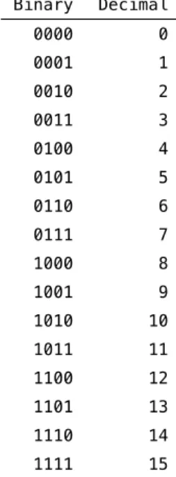
This is a 4-bit code since there are 4 binary digits. The full list of all values that can be represented using a 4-bit code are shown in Table 2.1.

So with a 4-bit binary code one can represent24 ₌ ₁₆_{different values (0-15).}

Each additional bit doubles the number of values one can represent. So a 5-bit code enables us to represent 32 distinct values, a 6-bit code 64, a 7-bit code 128

(22)

Binary Decimal

0000 0

0001 1

0010 2

0011 3

0100 4

0101 5

0110 6

0111 7

1000 8

1001 9

1010 10

1011 11

1100 12

1101 13

1110 14

1111 15

Table 2.1:Binary and decimal values for a 4-bit code.

and an 8-bit code 256 values (0-255).

Another piece of terminology: a given sequence of binary digits that forms the natural unit of data for a given processor (CPU) is called aword32_.

Have a look at theASCII table33_{. The standard ASCII table represents 128}

differ-ent characters and the extended ASCII codes enable another 128 for a total of 256 characters. How many binary bits are used for each?

2.2 Hexadecimal

You will also see in the ASCII table that it gives the decimal representation of each character but also the Hexadecimal and Octal representations. The hex-adecimal34_{system is a base-16 code and the}_octal35_{system is a base-8 code. Hex}

values for a single hexadecimal digit can range over:

(23)

11 2.2. HEXADECIMAL

If we use a 2-digit hex code we can represent16∗16 =256distinct values. In computer science, engineering and programming, a common practice is to rep-resent successive 4-bit binary sequences using single-digit hex codes.

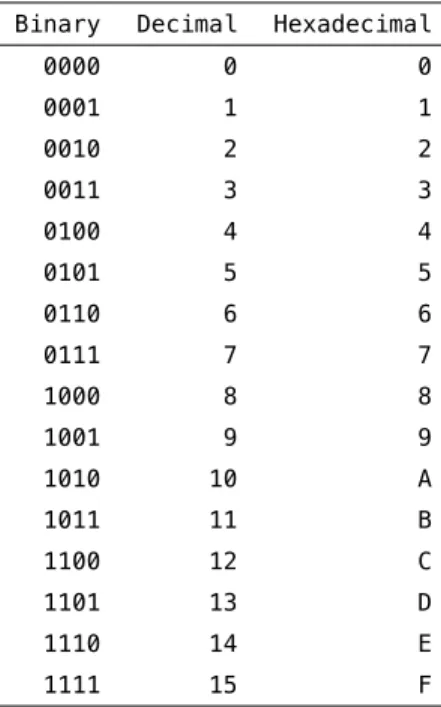
Table 2.2 shows 4-bit values of Binary, Decimal and Hexadecimal.

Binary Decimal Hexadecimal

0000 0 0

0001 1 1

0010 2 2

0011 3 3

0100 4 4

0101 5 5

0110 6 6

0111 7 7

1000 8 8

1001 9 9

1010 10 A

1011 11 B

1100 12 C

1101 13 D

1110 14 E

1111 15 F

Table 2.2:Binary, Decimal and Hexadecimal values for a 4-bit code.

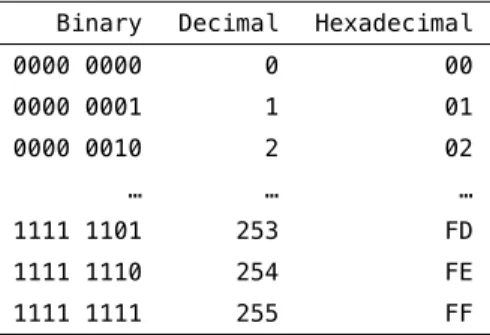
If we have 8-bit binary codes we would use successive hex digits to represent each 4-bit word of the 8-bitbyte36 _{(another piece of lingo). Table 2.3 shows}

how this would look for some 8-bit values in binary, decimal and hexadecimal.

The left chunk of 4-bit binary digits (the left word) is represented in hex as a single hex digit (0-F) and the next chunk of 4-bit binary digits (the right word) is represented as another single hex digit (0-F).

(24)

Binary Decimal Hexadecimal

0000 0000 0 00

0000 0001 1 01

0000 0010 2 02

… … …

1111 1101 253 FD

1111 1110 254 FE

1111 1111 255 FF

Table 2.3:Binary, Decimal and Hexadecimal values for an 8-bit (1-byte) code.

2.3 Floating point values

The material above talks about the decimal representation of bytes in terms of integer values (e.g. 0-255). Frequently however in science we want the ability to representreal numbers37_{on a continuous scale, for example 3.14159, or 5.5,}

or 0.123, etc. For this, the convention is to usefloating point38_{representations}

of numbers.

The idea behind the floating point representation is that it allows us to represent an approximation of a real number in a way that allows for a large number of possible values. Floating point numbers are represented to a fixed number of

significant digits(called asignificand) and then this is scaled using abaseraised to anexponent:

sxbe _(2.1)

This is related to something you may have come across in high-school science, namelyscientific notation39_{. In scientific notation, the base is 10 and so a real}

number like 123.4 is represented as1.234 x 102_.

In computers there are different conventions for different CPUs but there are standards, like theIEEE 75440 _{floating-point standard. As an example, a}

so-calledsingle-precision floating point format41_{is represented in binary (using a}

(25)

13 2.3. FLOATING POINT VALUES

is represented using 64 bits (8 bytes). In C you can find out how many bytes are used for various types using thesizeof()function:

#include <stdio.h>

int main(int argc, char *argv[]) {

printf("a single precision float uses %ld bytes\n", sizeof(float));

printf("a double precision float uses %ld bytes\n", sizeof(double)); return 0;

}

On my macbook pro laptop this results in this output:

a single precision float uses 4 bytes

a double precision float uses 8 bytes

According to the IEEE 754 standard, a single precision 32-bit binary floating point representation is composed of a1-bit sign bit(signifying whether the num-ber is positive or negative), an8-bit exponentand a23-bit significand. See the various wikipedia pages for full details.

There is a key phrase in the description of floating point values above, which is that floating point representation allows us to store anapproximationof a real number. If we attempt to represent a number that has more significant digits than can be store in a 32-bit floating point value, then we have to approximate that real number, typically by rounding off the digits that cannot fit in the 32 bits. This introducesrounding error42_.

Now with 32 bits, or even 64-bits in the case of double precision floating point values, rounding error is likely to be relatively small. However it’s not zero, and depending on what your program is doing with these values, the rounding er-rors can accumulate (for example if you’re simulating a dynamical system over thousands of time steps, and at each time step there is a small rounding error).

(26)

Python, R, C, etc) and type the following (adjust the syntax as needed for your language of choice):

(0.1 + 0.2) == 0.3

What do you get? In MATLAB I get:

>> (0.1 + 0.2) == 0.3

ans =

0

In MATLAB,0is synonymous with the logical valueFALSE. What’s going on here? What’s happening is that these decimal numbers, 0.1, 0.2 and 0.3 are being rep-resented by the computer in a binary floating-point format, that is, using a base 2 representation. The issue is that in base 2, the decimal number 0.1 cannot be represented precisely, no matter how many bits you use. Plug in the deci-mal number 0.1 into an online binary/decideci-mal/hexadecideci-mal converter (such as here43_{) and you will see that the binary representation of 0.1 is an infinitely}

re-peating sequence:

0.000110011001100110011001100... (base 2)

This shouldn’t be an unfamiliar situation, if we remember that there are also real numbers that cannot be represented precisely in decimal format, either, be-cause they involve an infintely repeating sequence. For example the real num-ber1₃ when represented in decimal44_is:

0.3333333333... (base 10)

(27)

15 2.4. ASCII

amount of precision that depends on how many significant digits we retain in our representation.

So the same is true in binary. There are some real numbers that cannot be rep-resented precisely in binary floating-point format.

Seehere45_{for some examples of significant adverse events (i.e. disasters) cause}

by numerical errors.

Rounding can be used to your advantage, if you’re in the business of stealing from people (seesalami slicing46_{). In the awesomely kitchy 1980s movie}

Super-man III47_{, Richard Pryor’s character plays a “bumbling computer genius” who}

embezzles a ton of money by stealing a large number of fractions of cents (which in the movie are said to be lost anyway due to rounding) from his company’s payroll (YouTube cliphere48_).

There is a comprehensive theoretical summary of these issues here:What Every Computer Scientist Should Know About Floating-Point Arithmetic49_.

Also see these webpages from the MathWorks online documentation about how MATLAB represents floating-point numbers:

Floating-Point Numbers50

and this section on avoiding common problems with Floating-Point Arithmetic:

Avoiding Common Problems with Floating-Point Arithmetic51

2.4 ASCII

ASCII stands forAmerican Standard Code for Information Interchange. ASCII codes delineate how text is represented in digital format for computers (as well as other communications equipment).

(28)

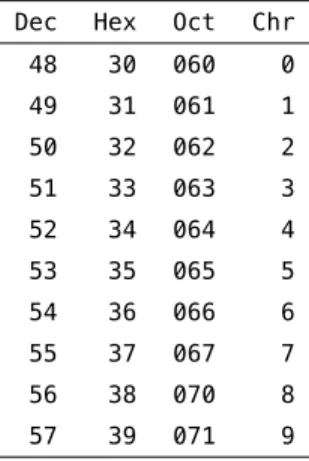
typical text symbols like#and&. Decimal codes 48 through 57 are the numbers

0through9. Decimal codes 65 through 90 are capital lettersAthroughZ, and

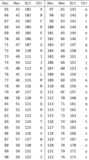
codes 97 through 122 are lowercase lettersathroughz. Table 2.4 shows codes in

decimal, hexadecimal and octal (base-8) for the numbers 0 through 9. Table 2.5 shows codes for uppercase and lowercase letters.

Dec Hex Oct Chr

48 30 060 0

49 31 061 1

50 32 062 2

51 33 063 3

52 34 064 4

53 35 065 5

54 36 066 6

55 37 067 7

56 38 070 8

57 39 071 9

Table 2.4:7-bit ASCII codes for the numbers 0 through 9.

For a full description of the 7-bit ascii codes in their entirety, including the ex-tended ASCII codes(where you will find things like ö and é), see this webpage:

http://www.asciitable.com52_{(ASCII Table and Extended ASCII Codes).}

In MATLAB, all individual text characters (variable typechar) are represented,

under the hood, as decimal ASCII values. Have a look at this code, in which we ask for the numeric value of individual characters. You can see that the result corresponds to their decimal ASCII values in Table 2.5.

>> double('a')

ans =

97

>> double('b')

(29)

17 2.4. ASCII

98

>> double('z')

ans =

122

You can get the character value of an ASCII code in MATLAB using thechar()

function:

>> char(65)

ans =

A

You can use your knowledge of ASCII codes to do tricky things in MATLAB, like convert to and from uppercase and lowercase, given your knowledge that the difference (in decimal) between ASCIIAand ASCIIais 32 (see Table 2.5).

>> char('A' + 32)

ans =

a

>> char('a' - 32)

ans =

(30)

Exercises

E 2.1 Convert the following decimal integer values into hexadecimal (resist the urge to use an online decimal–to–hex tool, try to do it using your brain):

1. 64206 2. 47806 3. 4013 4. 64222 5. 47802

E 2.2 Convert the following decimal integer values into binary (little-endian for-mat):

1. 2 2. 20 3. 200 4. 17 5. 170

E 2.3 Convert the following (little-endian) binary values into hexadecimal:

1. 0001 2. 1000 3. 1001 4. 1000 0001

(31)

19 LINKS

Links

29_{http://en.wikipedia.org/wiki/Binary_code}

30_{http://en.wikipedia.org/wiki/Bit}

31_{http://en.wikipedia.org/wiki/Endianness}

32_{http://en.wikipedia.org/wiki/Word_(computer_architecture)}

33_{http://www.asciitable.com}

34_{http://en.wikipedia.org/wiki/Hexadecimal}

35_{http://en.wikipedia.org/wiki/Octal}

36_{http://en.wikipedia.org/wiki/Byte}

37_{http://en.wikipedia.org/wiki/Real_number}

38_{http://en.wikipedia.org/wiki/Floating_point}

39_{http://en.wikipedia.org/wiki/Scientific_notation}

40_{http://en.wikipedia.org/wiki/IEEE_floating_point}

41_{http://en.wikipedia.org/wiki/Binary}₃₂

42_{http://en.wikipedia.org/wiki/Round-off_error}

43_{http://www.wolframalpha.com/input/?i=}₀_.₁_+to+binary

44_{http://www.wolframalpha.com/input/?i=}₁_%₂_F₃_+in+decimal

45_{http://ta.twi.tudelft.nl/users/vuik/wi}₂₁₁_{/disasters.html}

46_{http://en.wikipedia.org/wiki/Salami_slicing}

47_{http://en.wikipedia.org/wiki/Superman_III}

48_{http://www.youtube.com/watch?v=iLw}₉_OBV₇_HYA

49_{http://docs.oracle.com/cd/E}₁₉₉₅₇_-₀₁_/₈₀₆_-₃₅₆₈_{/ncg_goldberg.html}

50_{http://www.mathworks.com/help/matlab/matlab_prog/floating-point-numbers.html}

51_{http://www.mathworks.com/help/matlab/matlab_prog/floating-point-numbers.html#}

bqxyrhp

(32)

Dec Hex Oct Chr Dec Hex Oct Chr

65 41 101 A 97 61 141 a

66 42 102 B 98 62 142 b

67 43 103 C 99 63 143 c

68 44 104 D 100 64 144 d

69 45 105 E 101 65 145 e

70 46 106 F 102 66 146 f

71 47 107 G 103 67 147 g

72 48 110 H 104 68 150 h

73 49 111 I 105 69 151 i

74 4A 112 J 106 6A 152 j

75 4B 113 K 107 6B 153 k

76 4C 114 L 108 6C 154 l

77 4D 115 M 109 6D 155 m

78 4E 116 N 110 6E 156 n

79 4F 117 O 111 6F 157 o

80 50 120 P 112 70 160 p

81 51 121 Q 113 71 161 q

82 52 122 R 114 72 162 r

83 53 123 S 115 73 163 s

84 54 124 T 116 74 164 t

85 55 125 U 117 75 165 u

86 56 126 V 118 76 166 v

87 57 127 W 119 77 167 w

88 58 130 X 120 78 170 x

89 59 131 Y 121 79 171 y

90 5A 132 Z 122 7A 172 z

(33)

3 Basic data types, operators & expressions

3.1 Expressions

When you start MATLAB you are greeted with a command prompt:

>>

You are now in the_{and MATLAB is waiting for you to}

en-ter anexpression, so that MATLAB can evaluate that expression and provide you with the result. For example, you might enter something that looks like arith-metic:

>> 1+2

ans =

3

MATLAB evaluates that expression 1+2 and prints out the value of that expres-sion, which is 3, and assigns that output value to a newvariablecalledans. We

will talk about variables soon.

Try typing in another arithmetic expression, for example:

>> 1/3

ans =

(34)

0.3333

So you can see that MATLAB can do division too.

Expressions don’t have to be arithmetic. They could be logical expressions, such as:

>> 1+2 == 3

ans =

1

In this case the double-equal sign is anoperatorwhich means “is equal to?”. Es-sentially our expression is asking MATLAB a logical question (a question with a TRUE or FALSE answer): Is1+2equal to3? MATLAB evaluates that expression and returns the answer:1. In MATLAB a logical TRUE is the same as the number 1, and a logical FALSE is the same as the number0. Try another logical expres-sion:

>> 1+1 == 0

ans =

0

In this case we are asking MATLAB “Does 1+1 equal 0?” and MATLAB returns0,

which is MATLAB’s way of sayingFALSE.

Here’s another one in which we combine multiple operators into one expres-sion:

>> 5+6-1+20>25

(35)

23 3.1. EXPRESSIONS

1

With the numbers and operators all squished next to each other this is a bit hard to read. I might prefer to write this expression with spaces in between, and round brackets surrounding the left hand side, to make it more readable:

>> (5 + 6 - 1 + 20) > 25

ans =

1

It’s up to you how to write your code, but I would suggest to you that writing your code in such a way that it is easy to read is a good idea in the long run. It will make it easier for other people to read your code (including yourself in the future).

Here’s an example to illustrate this point. Can you figure out what the result of this expression is?

>> 2*6*3*4/3/4/2/5>1

It’s difficult and annoying to try to do this. How about this re-written version:

>> (2*6 * 3*4) / (3*4 * 2*5) > 1

ans =

1

They are both valid code, they both evaluate to the same result, but one version (the second version) is much more readable (in my opinion).

(36)

>> 0.1 + 0.2 == 0.3

ans =

0

This is a rather surprising result, isn’t it. I’ll leave it as an exercise for you to research why this happens, and what a potential solution to this kind of unex-pected result might be. Hint: look at the course notes ondigital representation of data54_.

Let’s move on and talk about operators.

3.2 Operators

In the example code snippets above we saw a number of operators already. We saw the +and /mathematical operators, and we saw the logical operator ==.

There are in fact a wide variety of operators in MATLAB. The MathWorks (the company that makes MATLAB) has a web page that lists them all:

Operators and Elementary Operations55

There are a variety of arithmetics operators, relational and logical operators, and others that you can read about as well.

One concept that is important to talk about isoperator precedence. This refers to the order in which MATLAB evaluates expressions and operators when there are multiple operations in a single expression. Take the following expression for example:

>> 2 + 3 * 5

(37)

25 3.3. VARIABLES

would evaulate to2+3, which is5, multiplied by5, which equals25. This is not

what happens in MATLAB (nor in most programming languages). Instead the multiply operator*takes precedence over the addition operator+, and the3*5

sub-expression is evaluated first, and then the result (which is15) is substituted,

and then the resulting expression2+15is evaulated, which returns17.

>> 2 + 3 * 5

ans =

17

Here is a page from the MathWorks documentation on MATLAB that describes operator precedence in MATLAB:

Operator Precedence56

For arithmetic the easy rule to remember is that multiply and divide take prece-dence over add and subtract.

You can force particular parts of an expression to be evaluated first by using round brackets, which take the highest precedence in MATLAB. For example we could rewrite the expression above to force the2+3to occur first, like this:

>> (2 + 3) * 5

ans =

25

3.3 Variables

(38)

store the results of your expression, MATLAB automatically stores the result in a variable calledans(short foranswer). So for example:

>> 1 + 2

ans =

3

MATLAB has stored the answer in avariablecalledans. You can think of a

vari-able as a human-readvari-able name of some data that is stored in MATLAB’s mem-ory. You can refer to data by it’s variable name. Under the hood, MATLAB keeps track of how these variable names correspond to the location (and type) of the data stored in memory.

This memory we are referring to is RAM orRandom-access memory57_{. This is}

a form of data storage in your computer which is to be considered temporary. Once MATLAB quits, or your computer is turned off, the data that was stored in RAM is gone. To permanently store data on your computer you need to store it on a more permanent form of memory, such as the hard drive in your computer, or an external drive such as a memory stick.

By naming your data using a variable name, you can easily view and manipulate those data. Here’s an example where we store the result of a calculation in a variable that we will namefred:

>> fred = 1 + 2

fred =

3

We type our expression1+2and on the left hand side we type our variable name

(39)

27 3.3. VARIABLES

fredis equal to3.

Here’s another one:

>> bob = 4 * 5

bob =

20

Now we have defined a second variable calledbobwhich we have set to be equal to the result of the expression4*5. We can see in MATLAB’s return statement that now bob is equal to20.

We can use variable names within expressions and MATLAB will substitute the value of those variables within the expression:

>> joe = bob + fred

joe =

23

We have defined a new variable calledjoeand assigned it to be equal to the value

ofbob(which is20) added to the value offred(which is3). MATLAB returns that

nowjoeis equal to23.

What happens if we do this?

>> mike = joe + bob + fred + danny Undefined function or variable 'danny'.

MATLAB returns an error:Undefined function or variable 'danny'. The problem here is that we have never defined a variable calleddannyand so when MATLAB attempts to evaluatedanny, it can’t find anything. When it evaluatesjoeandbob

(40)

have not named any data using a variable calleddannyand so MATLAB has no

idea what we are referring to.

In fact this is exactly the right way to think about this error: when we typedanny,

MATLAB does not know what we are referring to.

At any time we can get a list of which variables are defined in MATLAB by using a command calledwho:

Your variables are:

bob fred joe

We can see we have three variables defined. You can use a command calledwhos

to get a more detailed list:

>> whos

Name Size Bytes Class Attributes

bob 1x1 8 double

fred 1x1 8 double

joe 1x1 8 double

We see our variables in a table now with their name, their size, the number of Bytes that they occupy in MATLAB’s memory, their class (whattypeof variable they are, which relates to what kind of digital representation holds those data) and a column calledAttributes.

Note that if you assign a new value to an existing variable, the old data is wiped out. Here is an example. We first assign the number3to the new variablejane:

>> jane = 3

jane =

(41)

29 3.3. VARIABLES

Now we verify that indeedjaneis3:

>> jane

jane =

3

Now we reassign the number4tojane, and check the value:

>> jane = 4

jane =

4

>> jane

jane =

4

Indeed,janeis now4and there is no trace of3.

There are some rules governing how you can name your variables. Variable names cannot start with a number or a symbol, only with a letter. There can be no spaces or symbols in variable names. Capitalization matters, sojoeis dif-ferent thanJoe.

The other thing to talk about in this context is that MATLAB has some com-mands and functions that are already defined by MATLAB, and so you should avoid using those as your own variable names. So for example MATLAB has a built-in function calledsort()that will sort a vector of values:

>> sort([4 3 2 6 5 7 9 8 1])

(42)

1 2 3 4 5 6 7 8 9

When you typesortMATLAB executes its built-in sorting algorithm. Nothing

stops you however from defining your own variable with the same name:

>> sort = 23

sort =

23

Now when you try typing the sorting expression in again you get this:

>> sort([4 3 2 6 5 7 9 8 1]) Index exceeds matrix dimensions.

MATLAB throws an error. Now when MATLAB seessortit thinks you are

refer-ring to your variable calledsortwhich equals23. Actually it equals a1x1matrix

(a single value) containing23.

Why do we get this particular error message? The round brackets when put next to a variable cause MATLAB to try to index into a vector or matrix, and since our variable sort has only a single value, when MATLAB tries to retrieve the 4th, then 3rd, then 2nd, values, etc, it throws an error. We haven’t talked about vectors or matrices or indexing yet, so don’t worry about that. The point here is that we have essentially wiped out the reference to the sorting algorithm originally referred to by sort by defining our own variable calledsort. Oops!

We can remedy this situation by clearing the variablesortusing the built-in

com-mandclear:

(43)

31 3.4. BASIC DATA TYPES

Now we have erased our variable calledsortand when we typesortagain,

MAT-LAB will no longer refer to our variable containing23(since we just cleared it

from memory) and MATLAB will go back to referring to its own built-in func-tion calledsort():

>> sort([4 3 2 6 5 7 9 8 1])

ans =

1 2 3 4 5 6 7 8 9

Now it’s time to talk about variable types.

3.4 Basic Data Types

So far we have been dealing with data in the form of single numbers. The num-ber1for example, or the number0.5. There are in fact a number of different

numerictypesof data that MATLAB can store in variables. Here is a webpage from the MathWorks that describes the full constellation of data types used in MATLAB:

Data Types58

Numeric data can be stored in a number of differentNumeric Types59_{. The}

default type of numeric data in MATLAB isdouble, which stands for double-precision floating-point format60_{. The}_{floating-point} _{part of this means}

essen-tially that this data type can store areal number61_{, i.e. numbers along a}

contin-uous line such as1.0or1.33or3.14159. Thedouble-precisionpart of this refers to how manybytesare used by MATLAB to represent that number. More bytes means more precision. You can read about this in more detail in Chapter 2, Dig-ital representation of data.

(44)

>> a = 1

a =

1

>> b = 2

b =

2

>> c = a/b

c =

0.5000

>> d = b/a

d =

2

>> whos

a 1x1 8 double

b 1x1 8 double

c 1x1 8 double

d 1x1 8 double

If you want to convert a variable to another numeric data type, you can do it using one of MATLAB’s built-in conversion functions. So for example to convert adoublevariable to a 32-bit integer, useint32():

(45)

x =

1.3000

>> y = int32(x)

y =

1

>> whos

x 1x1 8 double

y 1x1 4 int32

You can see that when thedouble x(which equals1.3) is converted into anint32

it is rounded down to1.

MATLAB also has data types to deal with individual characters (letters like'a'

and'b') and strings of characters (like'joe'), and a selection of built-in func-tions to manipulate strings:

Characters and Strings62

For example:

>> x = 'a'

x =

a

>> y = 'b'

y =

(46)

>> z = 'fred'

z =

fred

>> whos

x 1x1 2 char

y 1x1 2 char

z 1x4 8 char

Above we have defined three variables all of typechar(which stands for charac-ter string). The first two, namedxandyboth contain a single character ('a'and

'b', respectively) and the third,z, contains a string of four characters ('fred'). You can see thatxandyoccupy 2 bytes of memory andzuses 8 bytes. Two bytes are required to store a single character in MATLAB.

You can dive deeper here in the documentation for thechar function63_{, which}

describes how characters are represented. The first 7 bits (values 0 to 127) code 7-bit ASCII characters. The next 9 bits code values 128 to 65535 and represent characters that depend on your locale (i.e. other languages besides plain english ASCII).

You can quickly see the integer codes for different characters in MATLAB by do-ing the followdo-ing:

>> int8('a')

ans =

97

>> int8('b')

(47)

98

>> int8('z')

ans =

122

In fact you can get the integer codes for all 26 lower case letters in one go, like this:

>> int8('a':'z')

ans =

Columns 1 through 15

97 98 99 100 101 102 103 104 105 106 107 108 109 110 111

112 113 114 115 116 117 118 119 120 121 122

You can display a string to the screen using thedispcommand:

>> disp('hello, world, my name is fred') hello, world, my name is fred

You can concatenate multiple strings using the square brackets[and]to

con-struct a new string:

>> a = 'fred'; >> b = 'joe';

>> c = 'jane';

>> s = ' ';

(48)

>> disp(z)

fred joe jane

I’ve introduced some new syntax here, the use of the semicolon;after an

ex-pression. This prevents MATLAB from echoing the value of the expression to the screen. The expression is still evaluated but MATLAB doesn’t echo the re-sult back to us on the screen. Use this when you want to suppress the output of expressions. If you don’t need to see the result of an expression on the screen then this makes for a cleaner MATLAB session.

You can get attributes of a string such as its length:

>> disp(['z is ', num2str(l), ' characters long']) z is 13 characters long

I’ve also introducted the built-in function num2str()which will convert a nu-meric type into a character string.

Another way to generate a character string out of many parts is to use the

sprintf()function. This mimics theprintf()function64_{that is famililar to C}

pro-grammers:

>> m = sprintf('z is %d characters long, & pi is approx. %.5f', l, pi);

>> disp(m)

z is 13 characters long, and pi is approximately 3.14159

The%dnotation tells the sprintf function that an integer numeric type will be

pro-vided here. The%.5fnotation says that a floating-point value will be provided,

and please show it using 5 decimal places. At the end of the string is where you supply the needed values, in the order in which they appear in the string. Note thatpiis a built-in value in MATLAB.

(49)

>> a = 3.14159

a =

3.1416

>> class(a)

ans =

double

You can use theisa()function to ask whether a variable is a certain type. For example:

>> isa(a,'char')

ans =

0

>> isa(a,'double')

ans =

1

Remember in MATLAB0is “FALSE” or “NO” and1is “TRUE” or “YES”.

So far we have seen numeric types and character string types. These are basic data types. MATLAB also allows for complex data types such as vectors, ma-trices, structures and cell arrays. These you can think of as container types, in other words data types that can store not just one value but many values.

(50)

as a vector of single characters.

In the next section in the notes we will talk about some of these complex data types and how to use them.

3.5 Special values

The MathWorks online documentation has a page on various special values built-in to MATLAB:

Special Values65

There is a special numeric value in MATLAB calledNaN(not a number). It is often

used to denote missing data.

There is also a special value calledInfwhich stands for infinity. Try typing the expression1/0and you will getInf.

There are other mathematical special values such aspi:

>> pi

ans =

3.1416

>> help pi

PI 3.1415926535897....

PI = 4*atan(1) = imag(log(-1)) = 3.1415926535897....

Reference page in Help browser

doc pi

and imaginary numbersiandj:

>> help i

I Imaginary unit.

(51)

39 3.5. SPECIAL VALUES

3+2*j and 3+2*sqrt(-1) all have the same value.

Since both i and j are functions, they can be overridden and used

as a variable. This permits you to use i or j as an index in FOR loops, etc.

3.6 Getting help

We can get help about MATLAB built-in commands and functions using thehelp

command:

(53)

41 3.6. GETTING HELP

WHO List current variables.

WHO lists the variables in the current workspace.

In a nested function, variables are grouped into those in the nested function and those in each of the containing functions. WHO displays

only the variables names, not the function to which each variable

belongs. For this information, use WHOS. In nested functions and in functions containing nested functions, even unassigned variables

are listed.

WHOS lists more information about each variable.

WHO GLOBAL and WHOS GLOBAL list the variables in the global workspace. WHO -FILE FILENAME lists the variables in the specified .MAT file.

WHO ... VAR1 VAR2 restricts the display to the variables specified. The

wildcard character '*' can be used to display variables that match a pattern. For instance, WHO A* finds all variables in the current

workspace that start with A.

WHO -REGEXP PAT1 PAT2 can be used to display all variables matching the

specified patterns using regular expressions. For more information on using regular expressions, type "doc regexp" at the command prompt.

Use the functional form of WHO, such as WHO('-file',FILE,V1,V2), when the filename or variable names are stored in strings.

S = WHO(...) returns a cell array containing the names of the variables

in the workspace or file. You must use the functional form of WHO when there is an output argument.

Examples for pattern matching:

who a* % Show variable names starting with "a"

who -regexp ^b\d{3}$ % Show variable names starting with "b" % and followed by 3 digits

who -file fname -regexp \d % Show variable names containing any

% digits that exist in MAT-file fname

See also WHOS, CLEAR, CLEARVARS, SAVE, LOAD.

(54)

Simulink.who

Reference page in Help browser

doc who

We can also get a GUI interface to help using thedoccommand.

There is also a way of searching the help documentation files for keywords, us-ing thelookforcommand. Thelookforcommand will return the names of all functions or commands for which the associated help documentation contains the given keyword. So for example let’s say we need to find theinvkine() func-tion but we’ve forgotten what it’s called, we just remember it’s something to do with a robot. We can search using:lookfor robot

>> lookfor robot

invkine - Inverse kinematics of a robot arm.

invkine_codepad - Modeling Inverse Kinematics in a Robotic Arm

idnlgreydemo13 - Modeling an Industrial Robot Arm

idnlgreydemo8 - Industrial Three-Degrees-of-Freedom Robot: C

MEX-File Modeling of MIMO System Using Vector/Matrix Parameters

robot_m - A simplified Manutec r3 robot with three

arms.

robotarm_m - A physically parameterized robot arm.

refmodel_dataset - ROBOTARM_DATASET Reference model dataset

robotarm_dataset - Robot arm dataset

mech_robot_data - Data defining the manutec robot.

RobotArmExample - Multi-Loop PID Control of a Robot Arm

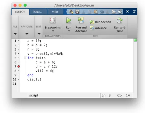
3.7 Script M-files

(55)

43 3.8. MATLAB PATH

So for example you might have a file calledrandom8.mthat contains the following

code:

% script M-file example random8.m

%

rlist = round(rand(1,8)*10);

disp(rlist);

disp(['mean = ',num2str(mean(rlist))]);

disp(['median = ',num2str(median(rlist))]);

disp(['standard deviation = ',num2str(std(rlist))]);

The script generates a list of 8 random numbers chosen from a uniform distri-bution between 0 and 10, and then displays the mean, median and standard deviation of those values.

If the script file calledrandom8.mis in your MATLAB path, then typingrandom8.m

on the MATLAB command line will execute the script:

>> random8

8 9 1 9 6 1 3 5

mean = 5.25 median = 5.5

standard deviation = 3.3274

3.8 MATLAB path

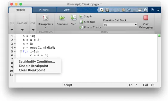
When you first start MATLAB, you will be faced with the command line prompt, and MATLAB will be started up looking at a particular location in your file sys-tem. This location is known as thecurrent working directory. If you are using the MATLAB GUI (graphical user interface) you will see your current working directory displayed in a toolbar just above the command line. On my computer it shows as/Users/plg/Desktop. On your computer it will be something different.

(56)

pwdinto the command line:

>> pwd

ans =

/Users/plg/Desktop

When you type something into the command line, likerandom8, MATLAB will go through a number of steps to find out what you mean:

• israndom8defined as a variable in memory?

• israndom8defined as a function or script file or data file in MATLAB’s current

working directory?

• israndom8defined as a function or script file or data file somewhere else in

MATLAB’s path?

The MATLAB pathis a list of directories on your computer’s hard disk where MATLAB knows to look for scripts and functions. You can see what’s defined in your MATLAB path by typingpathat the MATLAB command line:

>> path

MATLABPATH

/Users/plg/Documents/MATLAB

/Applications/MATLAB_R2015a.app/toolbox/matlab/addons /Applications/MATLAB_R2015a.app/toolbox/matlab/addons/cef

/Applications/MATLAB_R2015a.app/toolbox/matlab/addons/fallbackmanager

/Applications/MATLAB_R2015a.app/toolbox/matlab/demos /Applications/MATLAB_R2015a.app/toolbox/matlab/graph2d

/Applications/MATLAB_R2015a.app/toolbox/matlab/graph3d /Applications/MATLAB_R2015a.app/toolbox/matlab/graphics

... ...

(57)

sub-45 3.8. MATLAB PATH

directories of the MATLAB main application directory. This is where all of MAT-LAB’s built-in functions and scripts are located, and where the various MATLAB toolbox code is located.

The other way to see (and alter) your MATLAB path is by using the MATLAB GUI. Typepathtoolon the MATLAB command line and you get a nice GUI interface

where you can scroll through all of the directories that are in your MATLAB path, you can delete some, add some, and change the order.

On the issue of the order: remember that MATLAB goes through its path in the order in which the directories appear in the path list. So if you have a function calledrandom8()defined in multiple places in your path, when you typerandom8

on the MATLAB command line, MATLAB will use the first one it finds in the path.

My personal approach to the MATLAB path is to basically never mess with it. Instead of adding data directories and script directories associated with my var-ious projects to the MATLAB path, instead I just start MATLAB from the appro-priate location when I am working on different projects.

To change the current working directory you can either click on the toolbar in the MATLAB GUI, or use thecdcommand on the MATLAB command line, for example:

>> cd /Users/plg/Documents/Research/projects/Heather_fMRI/

>> pwd

ans =

(58)

Exercises

E 3.1 Write a program to convert temperature values from Celsius to Fahrenheit according to the equation:

F= 9

5C+32 (3.1)

The program should as the user to input the temperature in Celsius, and then print out a sentence giving the temperature in Fahrenheit, like this:

enter the temperature in Celsius: 22

22.0 degrees Celsius is 71.6 degrees Fahrenheit

E 3.2 Given parabolic flight, the height of a ball y is given by the equation:

y=xtan(θ)−

[

1 2v2

0

] [

gx2 cos(θ)2

]

+y0 (3.2)

wherexis a horizontal coordinate (metres),gis the acceleration of gravity (metres per second per second),v0is the size of the initial velocity vector

(metres per second) at an angleθ(radians) with the x-axis, and(0,y0)is

the initial position of the ball (metres).

Write a program to compute the vertical height of a ball. The program should ask the user to input values forg,v0,θ,x, andy0, and print out a

sentence giving the vertical height of the ball.

Test your program with this example:

enter a value for g: 9.8 enter a value for v0: 6.789

enter a value for theta: 0.123 enter a value for x: 4.5

enter a value for y0: 5.4

(59)

47 3.8. MATLAB PATH

E 3.3 As an egg cooks, the proteins first denature and then coagulate. When the temperature exceeds a critical point, reactions begin and proceed faster as the temperature increases. In the egg white the proteins start to coagulate for temperatures above 63 C, while in the yolk the proteins start to coagu-late for temperatures above 70 C. For a soft-boiled egg, the white needs to have been heated long enough to coagulate at a temperature above 63 C, but the yolk should not be heated above 70 C. For a hard-boiled egg, the centre of the yolk should be allowed to reach 70 C.

The following equation gives the timetit takes (in seconds) for the centre of the yolk to reach the temperatureTy(Celsius):

t= M

2/3_cρ1/3

Kπ2₍₄_π/₃₎2/3ln

[

0.76To−Tw

Ty−Tw ]

(3.3)

where M,ρ, candK are properties of the egg: M is mass, ρ is the den-sity,cis the specific heat capacity, andKis the thermal conductivity. Rel-evant values are M = 47g for a small egg andM = 67g for a large egg,

ρ=1.038g cm−3_,_c₌₃_.₇_{J g}−1_K−1_{, and}_K₌₀_.₀₀₅₄_{W cm}−1_K−1_{. The}

param-eterTwis the temperature (in Celsius) of the boiling water, andTois the

original temperature of the egg before being put in the water.

Implement the equation in a program, setTw = 100C andTy = 70C, and

computetfor a large egg taken from the fridge (To =4C) and from room

temperature (To=20C).

Test your program with this example:

Is the egg large (1) or small (0)? 1 enter the initial temperature of the egg

reminder 4.0 for fridge, 20.0 for room: 15.0

(60)

Links

53

54_{file:digital_representation_of_data.html}

55_{http://www.mathworks.com/help/matlab/operators-and-elementary-operations.html}

56_{http://www.mathworks.com/help/matlab/matlab_prog/operator-precedence.html}

57_{https://en.wikipedia.org/wiki/Random-access_memory}

58_{http://www.mathworks.com/help/matlab/data-types_data-types.html}

59_{http://www.mathworks.com/help/matlab/numeric-types.html}

60_{https://en.wikipedia.org/wiki/Double-precision_floating-point_format}

61_{https://en.wikipedia.org/wiki/Real_number}

62_{http://www.mathworks.com/help/matlab/characters-and-strings.html}

63_{http://www.mathworks.com/help/matlab/ref/char.html}

64_{https://en.wikipedia.org/wiki/Printf_format_string}

(61)

4 Complex data types

In Chapter 3 we saw data types such asdoubleandcharwhich are used to rep-resent individual values such as the number1.234or the character'G'. Here we will learn about a number of complex data types that MATLAB uses to store mul-tiple values in one data structure. We will start with thearrayandmatrix—and in fact a matrix is just a two-dimensional array. What’s more, a scalar value (like

3.14) is just an array with one row and one column. We will also covercell arrays

andstructures, which are data types designed to hold different kinds of informa-tion together in a single type.

4.1 Arrays

Arrays are simply ordered lists of values, such as the list of five numbers:

1,2,3,4,5. In MATLAB we can define this array using square brackets:

>> a = [1,2,3,4,5]

a =

1 2 3 4 5

>> whos

a 1x5 40 double

We can see thatais a1x5(1 row, 5 columns) array ofdoublevalues.

(62)

We can also get the length of an array using thelengthfunction:

>> length(a)

ans =

5

We can in fact leave out the commas if we want, when we construct the array— we can use spaced instead. It’s up to you to decide which is more readable.

>> a = [1 2 3 4 5]

a =

1 2 3 4 5

MATLAB has a number of built-in functions and operators for creating arrays and matrices. We can create the above array using a colon (:) operator like so:

>> a = 1:5

a =

1 2 3 4 5

We can create a list of only odd numbers from 1 to 10 like so, again using the colon operator:

>> b = 1:2:10

b =

(63)

51 4.1. ARRAYS

4.1.1 Array indexing

We can get the value of a specific item within an array byindexinginto the array using round brackets(). For example to get the third value of the arrayb:

>> third_value_of_b = b(3)

third_value_of_b =

5

To get the first three values ofb:

>> b(1:3)

ans =

1 3 5

We can get the 4th value onwards to the end by using theendkeyword:

>> b(4:end)

ans =

7 9

Remember, array indexing in MATLAB starts at 1.In other languages like C and Python, array indexing starts at 0. This can be the source of significant confu-sion when translating code from one language into another.

Another useful array construction built-in function in MATLAB is thelinspace

function:

>> c = linspace(0,1,11)

(64)

Columns 1 through 8

0 0.1000 0.2000 0.3000 0.4000 0.5000 0.6000 0.

7000

0.8000 0.9000 1.0000

By default arrays in MATLAB are defined as row arrays, like the arrayaabove

which is size1x5—one row and 5 columns. We can however define arrays as

columns instead, if we need to. One way is to simply transpose our row array using the transpose operator':

>> a2 = a'

a2 =

1

2 3

4 5

>> size(a2)

ans =

5 1

Now we can seea2is a5x1column array.

We can directly define column arrays using the semicolon;notation instead of commas or spaces, like so:

(65)

53 4.1. ARRAYS

a2 =

1 2

3

4 5

So in general, commas or spaces denote moving from one column to another, and semicolons denote moving from one row to another. This will become use-ful when we talk about matrices (otherwise know as two-dimensional arrays).

4.1.2 Array sorting

MATLAB has a built-in function calledsort() to sort arrays (and other

struc-tures). The algorithm used by MATLAB under the hood is thequicksort66

al-gorithm. To sort an array of numbers is simple:

>> a = [5 3 2 0 8 1 4 8 5 6]

a =

5 3 2 0 8 1 4 8 5 6

>> a_sorted = sort(a)

a_sorted =

0 1 2 3 4 5 5 6 8 8

If you give thesortfunction two output variables then it also returns the indices

corresponding to the sorted values of the input:

>> [aSorted, iSorted] = sort(a)

(66)

0 1 2 3 4 5 5 6 8 8

iSorted =

4 6 3 2 7 1 9 10 5 8

TheiSortedarray contains the indices into the original arraya, in sorted order. So

this tells us that the first value in the sorted array is the 4th value of the original array; the second value of the sorted array is the 6th value of the original array, and so on.

The default sort happens in ascending order. If we want to reverse this we can specify this as an option to thesort()function:

>> sort(a, 'descend')

ans =

8 8 6 5 5 4 3 2 1 0

4.1.3 Searching arrays

We can use MATLAB’s built-in function calledfind()to search arrays (or other

structures) for particular values. So for example if we wanted to find all values of the above arrayawhich are greater than 5, we could use:

>> ix = find(a > 5)

ix =

5 8 10