Nault_unc_0153D_17116.pdf

CONTINUUM-KINETIC MODELS AND NUMERICAL METHODS FOR MULTIPHASE APPLICATIONS

Isaac Michael Nault

A dissertation submitted to the faculty at the University of North Carolina at Chapel Hill in partial fulfillment of the requirements for the degree of Doctor of Philosophy in the Department of

Mathematics in the College of Arts and Sciences.

Chapel Hill 2017

ABSTRACT

Isaac Michael Nault: Continuum-Kinetic Models and Numerical Methods for Multiphase Applications

(Under the direction of Sorin Mitran)

This thesis presents a continuum-kinetic approach for modeling general problems in multiphase solid mechanics. In this context, a continuum model refers to any model, typically on the macro-scale, in which continuous state variables are used to capture the most important physics: conservation of mass, momentum, and energy. A kinetic model refers to any model, typically on the meso-scale, which captures the statistical motion and evolution of microscopic entitites. Multiphase phenomena usually involve non-negligible micro or meso-scopic effects at the interfaces between phases. The approach developed in the thesis attempts to combine the computational performance benefits of a continuum model with the physical accuracy of a kinetic model when applied to a multiphase problem.

ACKNOWLEDGEMENTS

I want to start by acknowledging the role of my family in my life. My parents, Michael and Carol, my brother, Josh, and my sister, Rachel, are the most important people in my life. They’ve loved and supported me through everything and I know that will never change. I wouldn’t be where I am in life if I didn’t have such a great family.

I would like to thank my advisor, Sorin Mitran, for all the teaching and guidance he has provided during my time at UNC. The classes he taught in my first few years were my favorite classes I took at UNC. Working with him was challenging at first, but it soon became a pleasure. Aside from offering invaluable insight on my project, I enjoyed the debates about future research direction that we had on many occasions. I don’t think there is a math professor at UNC who cares about his students’ well-being and future careers more than him.

During my time at UNC I’ve come to make some great lifelong friends from within the math department. These include Paul Cornwell and Travis McElroy. My time at UNC was much more enjoyable thanks to them.

In my third year at UNC I came to know Victor Champagne through some intermediate connections. He has become a career mentor for me. He has enabled many career opportunities for me in the past and future. I look forward to continuing work with him at the Army Research Lab after I graduate.

The last two summers I have spent interning at United Technologies Research Center in East Hartford, Connecticut. While there, my supervisor and mentor was Xuemei Wang. I want to thank her for all the work she did to make that a comfortable situation for me. Beyond endless paperwork required for me to work there, she was always available for questions and assistance.

TABLE OF CONTENTS

LIST OF FIGURES . . . ix

LIST OF TABLES . . . xi

LIST OF ABBREVIATIONS . . . xii

CHAPTER 1: INTRODUCTION . . . 1

1.1 Phases and Phase Transitions . . . 1

1.2 Scales of Description . . . 4

1.2.1 Micro-scale . . . 4

1.2.2 Macro-scale . . . 4

1.2.3 Meso-scale . . . 5

1.3 Equilibrium Phase Transition Models . . . 5

1.4 Micro-scale Numerical Simulations . . . 7

1.5 Multiphase Continuum Models . . . 8

1.5.1 Kinematic Descriptions . . . 10

1.5.2 Interface Capturing Methods . . . 11

1.5.3 Interfacial Boundary Conditions . . . 14

1.5.4 Deformation Gradients . . . 14

1.6 Kinetic Models . . . 17

1.7 Crystal Plasticity Methods . . . 18

1.8 Continuum-Kinetic Modeling Approach . . . 23

1.9 Cold Spray . . . 26

1.9.1 Cold Spray Modeling . . . 28

1.10 Outline . . . 32

2.1 Linear Elasticity . . . 33

2.1.1 Vector Form of System . . . 35

2.1.2 Eigenstructure . . . 36

2.2 Hyper-elasticity . . . 38

2.3 Lagrangian Hyper-elasticity . . . 40

2.3.1 Vector Form of System . . . 41

2.3.2 Eigenstructure . . . 43

2.4 Eulerian Hyper-elasticity . . . 45

2.4.1 Vector Form of System . . . 46

2.4.2 Eigenstructure . . . 47

2.5 Hyper-elastic Constitutive Laws . . . 50

2.5.1 Linear Elastic Constitutive Law . . . 51

2.5.2 Compressible Constitutive Law . . . 52

2.6 Eulerian Hyper-elastoplasticity . . . 53

2.6.1 Vector Form of System . . . 55

2.6.2 Eigenstructure . . . 55

2.7 Macro-scale Plastic Closures . . . 57

2.7.1 Perfect Plasticity . . . 58

2.7.2 Johnson-Cook Plasticity . . . 58

2.8 Crystal Plasticity Models . . . 59

2.8.1 Non-transportive Model . . . 59

2.8.2 Transportive Model . . . 64

CHAPTER 3: NUMERICAL METHODS . . . 68

3.1 Finite Volume Methods with Riemann Solvers . . . 68

3.1.1 Linear Systems . . . 71

3.1.2 Approximate Riemann Solvers . . . 72

3.1.3 Roe Linearization . . . 73

3.1.4 2nd Order Wave Propagation Scheme . . . 74

3.3 Macro-scale Plastic Correction . . . 76

3.4 Ghost Fluid Method . . . 78

3.4.1 Vacuum Boundaries . . . 81

3.4.2 Slip Boundaries . . . 82

3.4.3 Rigid Wall Boundaries . . . 83

3.5 Meso-scale Plastic Correction . . . 84

CHAPTER 4: MODEL VALIDATION . . . 88

4.1 Reflection Coefficients . . . 88

4.1.1 Theoretical Reflection Coefficients . . . 88

4.1.2 Numerical Results . . . 92

4.1.3 Vacuum Reflection Comparison . . . 93

4.1.4 Rigid-wall Reflection Comparison . . . 95

4.2 Convergence . . . 97

CHAPTER 5: COLD SPRAY MODELING . . . 101

5.1 Johnson-Cook Simulations . . . 102

5.2 Crystal Plasticity Simulations . . . 103

5.3 Model Comparison . . . 105

CHAPTER 6: CONCLUSION . . . 112

LIST OF FIGURES

1.1 Unary phase diagram of pure iron [1]. Solid-state iron exhibits both face-centered-cubic

(fcc), body-centered-cubic (bcc), and hexagonal-close-packed (hcp) crystal structure . . . 2

1.2 Conceptual interpretation of continuum variables. Non-moving particles have a zero average momentum and energy (left). Moving particles with no particular order have low average momentum and large internal energy (middle). Moving particles with high order have large average momentum and low internal energy (right) . . . 9

1.3 Conceptual interpretation of ’intermediate’ or ’current equilibrium’ configuration [2] . . 16

1.4 Instances of micro-states in which a continuum description fails to capture important information. A small number of particles inside the representative volume (left). A slip in a crystal lattice structure (right) . . . 17

1.5 FCC unit cell (a), principal directions (b), arrangement of atoms in close-packed plane (c), stacking sequence (d) [3] . . . 19

1.6 Undeformed crystal lattice (a), edge dislocation (b), screw dislocations (c,d) [3] . . . 21

1.7 Adaptive mesh refinement hones in on phase interface . . . 25

1.8 Crossection of a copper particle embedded in an Al 7050 substrate [4] . . . 26

1.9 Jetting phenonmenon in CS single particle impact [5] . . . 28

1.10 EBSD image of cold-sprayed Al 6061 crossection [6] . . . 29

4.1 Vacuum boundary reflection,θ=arctan(1/4) . . . 93

4.2 Vacuum boundary reflection,θ=arctan(1/3) . . . 93

4.3 Vacuum boundary reflection,θ=arctan(1/2) . . . 94

4.4 Theoretical and numerical vacuum boundary reflection coefficients . . . 94

4.5 Rigid-wall boundary reflection,θ=arctan(1/4) . . . 95

4.6 Rigid-wall boundary reflection,θ=arctan(1/3) . . . 95

4.7 Rigid-wall boundary reflection,θ=arctan(1/2) . . . 96

4.8 Theoretical and numerical rigid-wall boundary reflection coefficients . . . 96

4.9 ∆x= 2µm resolution . . . 97

4.10 ∆x= 1µm resolution . . . 97

4.11 ∆x= 0.5µm resolution . . . 98

4.12 ∆x= 0.25µm resolution . . . 98

4.13 1D slices at various resolutions . . . 99

5.1 Time slices of JC impact simulation at 600 m/s. von Mises stress shown in color (MPa) 107 5.2 JC impact simulations at 200, 400, and 600 m/simpact speeds. von Mises stress shown

in color (MPa). Time slices taken near moment of elastic rebound . . . 108 5.3 Time slices of CP impact simulation at 600 m/s. von Mises stress shown in color (MPa) 109 5.4 Time slices of CP impact simulation at 600 m/s. Total immobile dislocation density

shown in color (1/µm2_{) . . . 110}

LIST OF TABLES

3.1 Various types of limiter functions . . . 75

5.1 Material properties used for Aluminum 6061 . . . 102

5.2 JC parameters for Aluminum 6061 . . . 102

LIST OF ABBREVIATIONS

ALE Arbitrary Lagrangian-Eulerian. 11

CP Crystal plasticity. 18–25, 32, 59, 84, 85, 102–106, 112, 113

CS Cold Spray. 26–32, 101, 112, 113

FV Finite Volume. 68–70

GFM Ghost Fluid Method. 14

JC Johnson-Cook. 58, 102–106, 113

MD Molecular Dynamics. 7, 32, 113

MGFM Modified Ghost Fluid Method. 14, 78, 102

CHAPTER 1 Introduction

Multiphase interactions represent some of the most common modeling challenges that arise in Engineering and the Sciences. Consequently, the solutions to multiphase problems are of great interest in a wide range of fields. This thesis develops a general approach for modeling and simulating multiphase interactions in solid-mechanics applications. A particular focus of the thesis is the use of models and methods at multiple scales of description. Therefore, one of the important original contributions of this thesis arises from the linking together of various models on different scales. As will be seen, this linking requires certain additional modeling, numerical, and implementation techniques as well as the consideration of theoretical complications arising from scaling. The approach has been motivated by a specific class of problems that have important physical phenomena on multiple scales of description. The thesis will consider metal grain recrystalization under large plastic deformation as an example. However, before proceeding in any manner, it will be beneficial to briefly discuss basic multiphase theory and the historical development of multiphase models. Doing so will provide some motivation for the approach that is the subject of this thesis.

1.1 Phases and Phase Transitions

First, it is necessary to define what is meant by the word phase. There are many possible interpretations. From the perspective of this thesis, a phase is a group of molecules large enough in number to be considered a macroscopic entity (see section 1.2.2) that behave collectively, and on average, in some predictable way. The most obvious phases are those distinguished by chemical composition; in other words, a single material may be considered a phase. More generally, a single material can itself have many phases: gas or liquid, for example; or the various lattice configurations of a solid. These types of phases are distinguished from one another by phase transitions: either first-order or continuous.

one in which the thermodynamic state variables that describe the system exhibit a discontinuity at the critical point of the phase transition. With few exceptions, the transitions between gas, liquid, solid and plasma are all considered first-order phase transitions.

On the other hand, a continuous phase transition does not involve any latent heat. As the name suggests, the state variables describing the system remain continuous across the transition. Mathematically, the feature which defines the phase transition is a discontinuity or divergence in any of the rates-of-change of the state variables. Examples of continuous phase transitions include the changes in crystal lattice structure of solid-state metal (see figure 1.1).

Figure 1.1: Unary phase diagram of pure iron [1]. Solid-state iron exhibits both face-centered-cubic (fcc), body-centered-cubic (bcc), and hexagonal-close-packed (hcp) crystal structure

In multiphase interactions it is common to define mathematical quantities that distinguish one phase from another. These quantities are called order parameters [7]. Typically, the order paramater is chosen in such a way that it is zero on one side of a phase transition and nonzero on the other. The order parameter is also a direct function of certain system variables. Therefore, the name ’order parameter’ is actually a misnomer; it is not a paramater, but rather a variable. In models, the order parameters provide a useful way to track where various phases are present in space at any given time. An example [7] of an order parameter is

for liquid-gas transitions. In this order parameter, ρ is the total particle density and ρgas is the density of gas as derived from the measured temperature and pressure. In a small control volume, the order parameter is zero if the volume is completely filled by particles in gas state. The order parameter is exactly equal to the total density if the control volume is completely filled by particles in liquid state. If there is a liquid-gas phase transition occuring within the control volume, the order parameter is somewhere in between zero and the total density.

In a discussion of phase transitions, it is important to discuss the use of thermodynamic potentials [8]. Thermodynamic potentials are functions whose rates-of-change with respect to thermodynamic variables encode all the necessary information to describe a system. In the context of phase transitions, the most common potentials are the Helmholtz and Gibbs free energies, which are functions of temperature and one other system-dependent variable. For a given system, at least one of these energies must be a function of only intensive variables, that is variables which do not depend on the size of the system. This particular free energy determines when a phase transition is in equilibrium: when the free energy of one phase is equal to that of the other.

Thermodynamic potentials provide a precise way to mathematically define 1st and higher order phase transitions. A first-order phase transition is defined as any point in state space where the first derivative of a chemical potential is discontinuous. Annth-order phase transition is defined where anynth-order derivative is discontinuous or divergent. Allnth order phase transitions for n >1 are classified as continuous phase transitions because the first order derivatives, which can be related to system variables, are continuous. These definitions were first proposed by Ehrenfest [9].

In some modeling approaches, it is useful to define an extended free energy which, in addition to the two intensive variables, is a function of the order parameter. For given intensive variables, the extended free energy is minimized when the order parameter is at phase equilibrium. If defined properly, any multiphase system will tend to change in a way so to minimize the extended free energy with respect to the order parameter. Therefore, the free energy provides a nice mathematical formulation for defining the dynamics of the order parameter.

to have a model that is based on physical first-principles and thus requires minimal experimental calibration.

1.2 Scales of Description

In many cases, two distinct phases may be succesfully modeled on their own at the macro-scale while being distinguished from one another by features most prominent on the scale of individual molecules, also known as the micro-scale. Before discussing this statement, it is necessary to define what is meant by these terms ’micro’ and ’macro’ scale. In addition, there is a third scale of interest in this thesis: the ’meso’ scale which is somewhere in between ’micro’ and ’macro’. The definition of these terms is usually qualitative. Further, the definition is usually problem-dependent, meaning what constitutes the micro-scale for one problem may be entirely different for another problem.

A somewhat more quantitative approach to distinguishing scales utilizes dimensionless numbers. One, the Knudsen number [11], is defined as the ratio of the mean free path to some representative length scale of the problem. The Knudsen number can be used to determine when the assumptions of a macroscopic model should begin to break down and a smaller-scale model should be used instead. A macro-scale model is considered valid when the Knudsen number is much less than one.

1.2.1 Micro-scale

The micro-scale is the scale of individual molecules. Historically speaking, the micro-scale is the scale of objects which are too small for the un-aided human eye to see [12]. This thesis takes the more mathematical perspective that the micro-scale is the scale at which the states of a system are, by necessity, modeled discretely as opposed to continuously. This discrete modeling is necessitated by the possiblity of thermal averages with large variance. Models on the micro-scale include Monte Carlo methods and MD methods.

1.2.2 Macro-scale

Historically, the macro-scale is the scale of objects visible to the un-aided human eye. A mathematical definition of macro-scale can be obtained in the following way. Let N be the number of particles in a system andV the volume occupied by the particles. The macro-scale is the scale of analysis in the thermodynamic limit N → ∞, V → ∞ [13]. Consider a cubic volume with sides∆x. Then, the number of particles in the system is given by N =NAρ∆x3/M whereNA is Avagadro’s

large for spatial scales∆x visible to the naked eye. On the macro-scale,N is generally considered so large that the states of the system can be represented by continuous functions. This assumption is valid because, whenN is sufficiently large, thermal averages of the state are expected to have negligible variance.

1.2.3 Meso-scale

The scale is somewhere in between the micro and macro-scale. Mathematically, the meso-scale can be viewed as sharing properties of the micro and macro-meso-scale. Like the micro-meso-scale, physical phenomena modeled on the meso-scale are expected to have non-negligible variance around the thermal averages [14]. Like the macro-scale, the number of particles in a meso-scale system is large enough that the states of the system may be modeled continuously, rather than discretely. Thus, a meso-scale system is one that is relatively large yet still exhibits non-equilibrium thermodynamics. The exact spatial range within which a meso-scale model should be defined depends on the physics of the problem at hand.

1.3 Equilibrium Phase Transition Models

Some of the simplest phase transition models are those based on the micro-scale in the realm of classical thermostatistics. These models are not dynamic. Rather, they assume thermodynamic equilibrium and are only capable of giving thermal averages of macroscopic quantities for a multiphase system. Therefore, these models are not practical for obtaining useful solutions to real-world problems. However, they do provide insight on the development of more sophisticated multiphase models. The models described in this section are based on particles that are confined to a cubic lattice and have a single scalar order parameter [7] defined at each lattice site.

The Ising model [15] was one of the earliest models of phase transition in a system. This model was designed to model the transition of a metal from ferromagnetic to paramagnetic. However, the order parameter of the model can be modified to treat other types of phase transitions. In the model, the order paramatersi at each lattice site, labelled byi, takes the value of1 or−1. In the magnetic

sense,si can be thought of as the direction of the spin. The Hamiltonian of the system is

H = 1 2

X

i,j

Jijsisj−B X

i

whereB can be interpreted as an imposed magnetic field, and

Jij = 

 

 

J if iand j are neighbors 0 otherwise

. (1.3)

IfJ <0, the model assigns lower energy, and thus higher probability, to states where neighboring spins are the same. IfJ >0 the model assigns lower energy to states where neighboring spins are opposite. Further, in either case, spins prefer to align with direction of the fieldB. The Ising model has solutions, that is thermal averages can be analytically obtained for useful quantities, in 1D [16] and in 2D [17] for the case ofB = 0.

The lattice-gas [18] is a model of a non-ideal gas, that is one in which molecules attract one another. The order parameter for the lattice gasei takes the value0 or 1, and represents whether a

lattice site is occupied by a molecule or not. No site is allowed to have more than one molecule and the total number of molecules must obviously remain constant. The Hamiltonian is given by

H= 2X

i,j

Jijeiej−µ X

i

ei (1.4)

where Jij is the same as in the Ising model. In this case, J <0. Therefore, the model assigns lower

energy to states in which molecules occupy neighboring sites. If the order parameter is replaced by

ei=

si+ 1

2 , (1.5)

it is seen that the lattice-gas model is mathematically equivalent to the Ising model.

The Heisenberg model [19] is a generalization of the Ising model to the case in which spins can point in any direction. Therefore, in this model the order parameter, −→si, is a vector. The

Hamiltonian is given by

H= 1 2

X

i,j

Jij−→si · −→sj −B~ · X

i

− →_s

i. (1.6)

~

B as closely as possible. Like the Ising model, the order parameters need not be interpreted as spins, but can have alternate physical interpretations for other types of phase transition models. TheXY model is a special name for the Heisenberg model for the particular case of two spatial dimensions. 1.4 Micro-scale Numerical Simulations

A simple, yet logical, idea for simulating a multiphase system is to evaluate exactly, or at least closely approximate, the thermal averages directly from the microscopic degrees of freedom. For a given micro-scale model of molecular behavior, the energy of each state is known, and therefore it is possible to compute any desired average. Of course, the problem is nearly all systems of interest have far too many degrees of freedom for an average to be computed in any reasonable time. The approach is to evaluate the averages by choosing a sampling of the microscopic state space that draws from the same distribution as the physical model (Gibbs distribution) [8],

p∼e−H/kT (1.7)

whereH is the Hamiltonian.

The use of random, or pseudorandom, numbers to achieve this is called a Monte Carlo method [20]. In particular, the Metropolis algorithm [21] generates a sequence of states drawn from the Gibbs distribution. The algorithm works by generating a new state from the current state and comparing the energies of each. If the new energy is less, the new state is accepted. If not, the new state is accepted with a probability proportional toexp(−∆E/kT), where∆E is the energy difference. After generating a large enough sequence of states, the desired averages are computed and assumed to be approximations of the true averages of the system.

An alternative approach is known as Molecular Dynamics (MD) [22, 23]. MD is any type of numerical solution of Newton’s equations of motion for all the molecules of the system. Succesful MD simulation relies on the assumption of ergodicity, that is, as a dynamical system evolves in time, states with equal energy are seen with equal likelihood. If a system is truly ergodic, the time average of the states explored by the simulation is equal to the same average in state-space. However, ergodicity is not always guaranteed. In some situations, an MD simulation will not sample all the equal-energy states fairly.

The resulting equations are known as the Langevin equations [24]. If the random noise is generated from a properly chosen distribution, the distribution of states satisfying the Langevin equations can be made to match the Gibbs distribution.

In general, the class of micro-scale methods can be very useful for certain problems. After all, these approaches are the closest thing to a truly first-principle model of a system. Furthermore, they can be insightful by generating solutions of so-called ’toy’ problems. These are problems that may not model a real-life scenario, but whose results could be used to inform a larger-scale model. Despite techniques for mitigating computational expense (most of which are not described here), micro-scale models are still generally limited to problems small in scale. For larger scale problems, models which project the complete micro-state onto some smaller degree-of-freedom state space are necessary in order for practical computation.

1.5 Multiphase Continuum Models

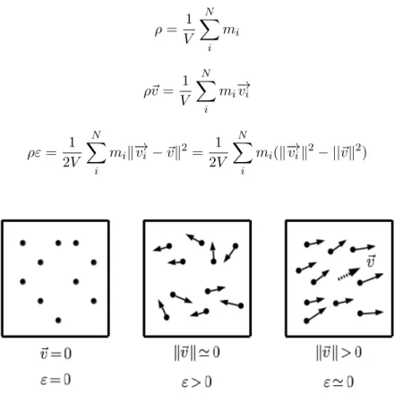
A continuum model is one way to drastically reduce the degrees of freedom of a model while still capturing the most important physical behavior. Continuum models are defined on the macro-scale and use state variables which are continuous in space and time. Conceptually, these variables can be viewed as the average of certain microscopic state variables inside a small volume immediately surrounding the point in space where the variable is defined. Mathematically, in order for the variables to be defined everywhere in space, the variables are interpreted as the limit of the arithemetic average of microscopic variables inside a volume as the volume goes to zero. However, in practice, numerical solutions of continuum models often discretize the domain into finite cells, and the state variables can be viewed as the averages over finite volumes.

ρ= 1 V

N X

i

mi (1.8)

ρ~v= 1 V

N X

i

mi−→vi (1.9)

ρε= 1 2V

N X

i

mik−→vi −~vk2 =

1 2V

N X

i

mi(k−→vik2− ||~vk2) (1.10)

Figure 1.2: Conceptual interpretation of continuum variables. Non-moving particles have a zero average momentum and energy (left). Moving particles with no particular order have low average momentum and large internal energy (middle). Moving particles with high order have large average momentum and low internal energy (right)

The backbone of continuum models are conservations laws. These are physical laws derived in integral form that come from consideration of the fluxes through the walls of an infinitesmal volume during an infinitesmal step in time. If the variables are assumed smooth, the conservation laws can be written in differential form. Actually, the conservation laws are usually presented in differential form even when the variables are not assumed to be smooth because the integral form can be easily derived from the differential form. The three most essential conservation laws are that of mass (1.11), momentum (1.12) and energy (1.13).

dρ

dt +ρ∇ ·~v= 0 (1.11)

ρd~v

dt − ∇ ·σ= 0 (1.12)

ρdE

Written in terms of stressσ, these equations are valid for any continuum, fluid or solid. Continuum models begin to diverge by the introduction of constitutive laws. Constitutive laws are most simply interpreted as equations which relate the stress with the other basic field variables. Constitutive laws can be derived in many ways most broadly categorized by: greatly simplified physical assumptions, experimental calibration of phenomenological equations, or equations derived from physical first principles. For instance, a greatly simplified assumption is that the stress can be divided into a ’hydrostatic’ part and a ’deviatoric’ part which is linearly proportional to the gradient of the velocity

and its transpose,

σ=−pI +µ(∇~v+∇~vT). (1.14)

Simplifying the momentum equation using this assumption yields the well known Navier-Stokes equations

ρd~v

dt +∇p=µ∇

2_{~v. (1.15)}

These equations still need one additional constitutive law to relate the pressure pto the other state variables. Thus it is seen that constitutive laws can also be viewed as the mathematically necessary closure of a system of equations.

When extending a continuum model to a multiphase system, the conservation laws are still valid for each of the system’s phases. However, the constitutive laws that close the equations for each phase could perhaps be different. Thus, the challenge with multiphase continuum methods is two-fold: how to track where each phase is present at any given time and how to deal with phase interaction at the interface. Many methods have been designed for dealing with both of these problems. Methods for tracking phase interfaces can be generally categorized by the reference frame used in the model. 1.5.1 Kinematic Descriptions

The Lagrangian reference frame is one whose reference grid follows the deformation of the material throughout time. The Lagrangian coordinates_X~ _{reference the material points that were} at_X~ _{in the initial configuration. The Eulerian reference frame is one whose reference grid is fixed} throughout time. Thus, Lagrangian and Eulerian reference systems are alternative ways of handling the same task. Lagrangian reference systems have a dynamic grid and fixed coordinatesdX~

dt = 0

. Eulerian reference systems have a fixed grid and dynamic coordinatesd~x

dt 6= 0

.

the materials. Therefore, in a multiphase model, so long as the initial nodes of the grid separate the phases exactly, the phase interfaces will be tracked explicitly by the evolution of the nodes. Thus, the issue of tracking phase interfaces in a Lagrangian model is trivial. This makes Lagrangian models appealing in many multiphase applications. However, if the deformations of the material are too large or complex, the Lagrangian grid can become convoluted, causing numerical techniques designed to solve the equations to become innacurate or computationally costly.

On the other hand, due to its fixed grid, an Eulerian model is much better suited to handling large or complex deformations. The downside is the evolution of the interface is no longer trivial to capture. Unlike a Lagrangian model, an Eulerian model must be able to have cells which contain multiple phases. Otherwise, an arbitrary interface would be impossible. Methods that evolve an interface on a fixed Eulerian grid are called interface capturing methods.

In addition to Eulerian and Lagrangian descriptions, a third type exists, the Arbitrary Lagrangian-Eulerian (ALE) description [25]. In an ALE description, the nodes of the grid are allowed to move, but not necessarily following the deformation of the underlying material. Rather, the motion is arbitrary, or perhaps prescribed to best suit the needs of the model. In particular, an ALE description can be used to optimize a multiphase model. In this case, the strategy is to choose a grid motion that follows phase interfaces exactly (Lagrangian) while being closer to stationary (Eulerian) in regions of the domain that are either far from phase interfaces or have large deformation. This strategy, if succesful, acquires the strengths of both Eulerian and Lagrangian descriptions for modeling multiphase systems. This thesis doesn’t explore ALE further. Nevertheless, ALE is recognized as a potential improvement to the modeling approach described ahead.

1.5.2 Interface Capturing Methods

of a new interface when an object splits. In these convoluted situations, a procedure for creating and removing markers is needed.

The remaining interface capturing methods sidestep the complexities of marker particles by introducing an additional field or fields to the system of equations. The computational work introduced by the new field comes as an acceptable cost of simpler and accurate capturing of complex interfacial motions. The earliest of such methods is the Volume of Fluid (VoF) method [27]. As its name suggests, the method works by tracking the fractional volume of one of the phases in each cell. Therefore, the value of this additional field variable should be 1 or 0 if the cell is one phase or the other, and somewhere between 1 and 0 if a phase interface passes through the cell. Further, the interface normal can be approximated by the gradient of the volume fraction in space. The volume fraction variableφevolves in time through advection by the background velocity field,

∂φ

∂t +~v· ∇φ= 0. (1.16)

The VoF method was originally designed for two-phase fluid problems, but is general enough to be used in any multiphase problem. For problems with more than two phases, additional volume fraction variables can be introduced to uniquely distinguish each phase.

The VoF and level set method each have their merits. Due to its use of a smooth function, unlike the step function used in VoF, the level-set method is better suited for numerical solutions of (1.16). On the other hand, if conservation of volume is a concern, a conservative numerical method applied to (1.16) will conserve volume if φis the volume fraction function. A further consideration is the fact that the signed-distance initialized level-set function carries additional useful information that the volume fraction does not. In some cases, in the application of boundary conditions, it is useful to know how far a cell is from the interface.

The phase-field method [30, 10] is a model of interface evolution inspired by the ideas of order parameters and extended free energies as discussed in section 1.1. A phase-field method, like VoF and level-set methods, uses a phase-indicator variable. In this case, the variable is interpreted as the order parameter of the phase transition. The order parameter is advected, but an additional source term is added to the evolution equation, yielding what is known as the Cahn-Hilliard equation,

∂φ

∂t +~v· ∇φ=κφ∇

2_{µ. (1.17)}

The source term is the Laplacian of the chemical potential µ, defined as the derivative of the free energyf with respect toφ,µ= ∂f_∂φ. Ifµis locally a monotonically increasing function of φ, (1.17) will drive φ in such a way so as to locally minimizef. This reveals the physical interpretation of the phase field model: the interface evolution is simultaneously determined by the motion of the background velocity and the minimization of free energy. This is a better model of what happens physically. Moreover, the phase-field method provides a direct way to introduce interfacial physical phenomena such as surface tension and miscibility through the definition off(φ). Other interface capturing methods cannot do this; interfacial physical phenomena must be accounted for in other ways with those methods. Numerically, phase-field methods are ideal because the interface can have finite width, thus avoiding the numerical issues associated with sharp interfaces.

towards phenomenological modeling. If, at the end of the day, the model relies on phenomenological modeling with experimental calibration, it is valid to ask why over-complicate the model in the first place. The addition of the source term in (1.17) requires additional numerical tools that aren’t necessary for VoF or phase-field methods.

1.5.3 Interfacial Boundary Conditions

Capturing the interface between phases is one problem. Implementing the proper interfacial conditions is another. In Lagrangian models, the boundary physics is somewhat simpler to implement. Since the nodes of the grid always follow the interface, surfaces of elements are always aligned with the interface as well. Therefore, the fluxes of certain quantities across the interface surfaces can be prescribed to match desired physical conditions as the simulation moves forward.

Implementation of internal boundary conditions in Eulerian models is less trivial. One approach makes use of ’ghost cells’, cells which are carefully prescribed at each time step to yield a desired effect in neighboring real cells after the numerical stencil of the method has been applied. This approach is known as the Ghost Fluid Method (GFM) [31]. GFM keeps a copy of state variables for each relevant phase in the simulation. An interface capturing method is used to identify which cells are ’inside’ or ’outside’ a given phase at all times. At the end of a time step, all ’outside’ cells within the radius of the scheme’s numerical stencil are repurposed as ghost cells. This procedure is repeated for each relevant phase, highlighting the need for multiple copies of the state data. The original GFM was designed for two-phase fluid problems, but the idea of using ghost cells can be extended to any multiphase problem, including solid-state problems. In [32], the prescription of ghost cell states was linked to the solution of the Riemann problem in a finite volume scheme. This method came to be known as the Modified Ghost Fluid Method (MGFM). In this strategy, the waves of the system which propagate outward from the interface are required to have zero magnitude, leaving only waves that propagate backwards from the interface. These constraints leave a small number of remaining degrees of freedom that can be used to prescribe precise interfacial conditions such as a jump in pressure in fluid-phase interactions or zero normal stress for a free boundary in solid mechanics. 1.5.4 Deformation Gradients

configuration~xwith respect to the coordinates in the initial configuration X~,

F = ∂~x

∂ ~X. (1.18)

The current configuration ~x is usually assumed to be related to the initial configurationX~ by a continuously differentiable field called the ’displacement’ ~u,

~

x=X~ +~u. (1.19)

Therefore, F can also be written as

F =I+ ∂~u

∂ ~X. (1.20)

The velocity field ~v which appears in (1.11-1.13) is formally defined as the time derivative of the displacement field~u, d_d~u_t =~v. Taking the time derivative of (1.20) yields

dF dt =

∂~v

∂ ~X =∇X~~v. (1.21)

In practice, (1.21) can included with (1.11-1.13) along with a constitutive law such as σ=σ(F) to form a complete dynamic system of equations. Such a model is known as a hyper-elastic model.

Crystalline solids are formed of molecules organized in a repeated pattern called a lattice. Lattice sites represent the ’equilibrium’ points around which molecules will oscillate under zero applied stress. Analogous to a one-dimensional spring, when a molecule is perturbed from its equilibrium position, one would expect the resulting force on the molecule to have some dependence on the coordinates of the ’equilibrium’ points. In a purely elastic solid, the initial coordinates _X~ _represent the equilbrium coordinates of the material points. Therefore, a constitutive law σ =σ(F) is the generalization of this principle to a continuum model. The force (σ·~ndA) on a material point is due to the current position (~x) of the material point relative to the local equilibrium points (X~) as captured by the gradient ∂~x

∂ ~X (F).

points by ~y. Then, by the argument of the previous paragraph, the stress at a point should only depend on the gradient of the current configuration with respect to the current equilibrium configuration,σ =σ

∂~x ∂~y

. This gradient is called the ’elastic’ portion of the deformation gradient Fe. It is clear that ~y(t) =X~ for alltis a necessary condition for a purely elastic deformation.

Assuming~yis a continuously differentiable function ofX, and using the chain rule, the deformation~ gradient F can be written

F = ∂~x ∂ ~X =

∂~x ∂~y

∂~y

∂ ~X =F

e ∂~y

∂ ~X. (1.22)

This decomposition suggests the ’plastic’ portion of the total deformation gradient is the gradient of the current equilibrium points with respect to the initial equilibrium points. This gradient can be denoted by Fp, leading to the so-called multiplicative decomposition [33, 34] of the deformation gradient

F =FeFp. (1.23)

This concept is illustrated in figure 1.3.

Figure 1.3: Conceptual interpretation of ’intermediate’ or ’current equilibrium’ configuration [2]

Let the assumed continuous dependence ofy~ onX~ be given by~y=X~+~up where~upis the ’plastic

displacement’. Further, let the plastic velocity be defined as~vp = d_d~u_tp. The plastic velocity gradient

Lp _{is defined as the gradient of the plastic velocity in the current equilibrium configuration (also}

called the lattice configuration)Lp₌ ∂~vp

∂~y. Lp is a useful variable in modeling because it describes

plastic deformation gradient by

Lp = ∂~vp ∂~y =

∂~vp

∂ ~X ∂ ~X

∂~y = dFp

dt F

p−1

. (1.24)

Therefore the dynamic evolution of Fp is given by

dFp

dt =L

p_Fp_{. (1.25)}

The dynamic equations (1.11, 1.12, 1.13, 1.21, 1.25) along with elastic constitutive lawσ=σ(Fe)and plastic constitutive law Lp =Lp(. . .)form a complete model of a non-linear elasto-plastic material. 1.6 Kinetic Models

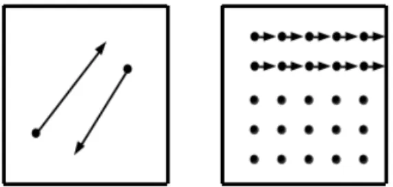
While being computationally practical, continuum models do not always accurately capture all information from a microscopic state. In particular, at a phase interface, the interaction of particles of each phase may not be accurately modeled by simply considering the macroscopic continuum states alone. Consider the scenarios illustrated in figure 1.4 using the same conventions as in figure 1.2.

Figure 1.4: Instances of micro-states in which a continuum description fails to capture important information. A small number of particles inside the representative volume (left). A slip in a crystal lattice structure (right)

In the right example, a ’slip’ is occuring on a crystal lattice. In a crystal lattice, slips may only occur along a finite set of slip directions. At low spatial resolution, the discrete nature of slip direction becomes effectively isotropic, and phenomonelogical ’plasticity’ models are used to capture the effects of slip. However, at high resolution, the discrete set of possible slip directions cannot be ignored due to the potentially high variance of slip along one direction with respect to other directions. This is especially relevant at a grain boundary, which could be considered a multiphase interface. At a grain boundary, the orientation of the crystal lattice differs from one side to the other. Therefore the possible slip directions also differ across this phase interface. If the resolution of the model is high enough such that the size of grains is large with respect to the size of finite cells, the effects of discretized slip direction will be non-negligible and a continuum model will be invalid. In the scenarios described above, the number of particles inside the representative volume may still be large enough that continuous variables are adequate to describe the state. The issue is the variance of the continuum state variables is expected to be potentially large. Clearly, this is the mesoscopic regime (section 1.2.3). In this thesis, models designed to capture physical phenomena like the ones described above are referred to as ’kinetic’ models. As will be seen, the name ’kinetic’ refers to the use of probabilistic distributions for the possible ’motions’ of model entities.

1.7 Crystal Plasticity Methods

The macro-scale phenomenon of plasticity observed in crystalline materials is fundamentally the result of micro-scale ’slips’ on the crystal lattice [3]. Crystal plasticity (CP) methods attempt to model plasticity by capturing the essence of this principle. CP models utilize continuous fields to capture non-equilibrium variances due to micro-scale physical phenomenon. Therefore, a CP model can be considered a meso-scale model or a kinetic model.

A slip within a crystal lattice can be mathematically characterized by two orthonormal vectors in space: the normal to the slip plane~nand the slip direction~s, also known as the normalized Burger’s vector. This pair of vectors is known as a ’slip system’. Due to the nature of a crystal lattice, only a finite set of slip systems may be uniquely defined. For example, the face-centered-cubic (FCC) crystal lattice has only 12 slip systems (see figure 1.5).

Figure 1.5: FCC unit cell (a), principal directions (b), arrangement of atoms in close-packed plane (c), stacking sequence (d) [3]

each slip system. Schmid’s law [35] defines the resolved shear stress τi on theith slip system as a

function of the applied stress σ and the unitary slip plane normal −→ni and slip direction−→si,

τi=σ:−→si ⊗ −→ni. (1.26)

The definition of resolved shear stress is common to all CP methods. The feature that distinguishes one CP method from another is a constitutive law that defines the shear rate on each slip system, denoted by γ˙i. The shear rate is usually defined as a function ofτi, a critical shear stress τic, and

possibly other slip system state variablesγ˙i= ˙γi(τi, τic, . . .). These constitutive laws may be either

phenomenological or physics-based. An illustrative example of a phenomenological constitutive law [2] is given by

˙ γi= ˙γ0

τi

τc i

1/m

sgn(τi), (1.27)

slip. The physical effect of (1.27) is apparent: the critical shear stress τ_icacts as the ’yield stress’ for the system i. When the resolved yield stress τi is small with respect to τ_ic the shear rate is close to

zero, and when τi is near or greater thanτic, the shear rate has non-negligible magnitude. In this

formulation,τ_ic is itself a dynamic variable which can be prescribed in such a way to empirically acount for hardening.

Physics-based constitutive laws in CP methods are typically based on internal variables related to the state of dislocations within the crystal lattice [2]. As stated above, plasticity is the result of slips along planes within a crystal lattice. However, slips of crystal planes do not usually extend across an entire crystalline object, or else the shear stresses required to cause a plastic deformation would be much higher than observed. Slips of crystal planes which terminate inside a crystal lattice must be accomodated by ’dislocated’ molecules. These are molecules which reside in non-equilbrium positions relative to the local crystal lattice in order to allow an overall energetically preferable state, such as a finite-length slip. Dislocations are the mathematical characterization of this phenomenon. A dislocation is the border of an area between two crystal planes which have been shifted with respect to one another [3]. For a dislocation caused by a slip on a crystal lattice, a segment of the dislocation can be uniquely distinguished by the slip plane normal~n, slip direction~sand the line direction~l, defined as the tangent vector to the dislocation at that point. The dislocation segment is characterized by the orientation of the slip direction with respect to the line direction (see figure 1.6). Where the line direction is perpendicular to the slip direction (~l·~s= 0), the dislocation is characterized as ’edge’ dislocation. Where the line direction is parallel to the slip direction (~l·~s= 1), the dislocation is characterized as ’screw’ dislocation. Everywhere else the dislocation has ’mixed’ character.

Figure 1.6: Undeformed crystal lattice (a), edge dislocation (b), screw dislocations (c,d) [3]

Physics-based constitutive laws define the dependence of the shear rate on the dislocation densities in addition to the resolved shear stress [2],

˙

γi = ˙γi(τi, ρedge_i , ρscrewi , . . .). (1.28)

This constitutive law is supplemented by evolution equations for each type of dislocation density (1.29),

dρc_i

dt +∇ ·(ρ

c

i~vic) = Φci. (1.29)

Among other things, these evolution equations account for: transport of the dislocation density by the background motion of the medium dρc_i

dt , transport due to the motion of dislocations with

respect to the crystal lattice ∇ ·(ρc

i~vic), and the generation and annihilation of dislocations due to

plastic deformationΦc_i.

exchange information as needed. Compatible continuum models must account for the elastic and plastic parts of the deformation gradient as defined in section 1.5.4. The CP model is linked to the continuum model by the plastic velocity gradient Lp,

Lp =X

i

˙

γi−→si ⊗ −→ni, (1.30)

and appears through (1.25). Equation (1.30) imposes the effect that the evolution of plastic deformation depends on the sum of contributions from each slip system and that this dependence comes through the definition of the shear rates on each system.

CP methods were not designed with multiphase problems in mind. Yet, they can be easily extended to modeling the multiphase problem of grain interaction with some simple modifications. As discussed in section 1.5.4, the elastic part of the deformation gradientFe _{is the mapping from the}

lattice configuration to the current configuration. Therefore, the orientation of crystal grains can be captured byFe. In particular, by QR decomposition,Fecan be computed as the productFe=OTU where O is an orthonormal matrix. For rotationally invariant constitutive laws, the dependence of the stress on Fe should come through U alone, σ(Fe) =σ(U). Thus,O can interpreted as the crystal orientation and U the ’elastic stretch tensor’, the piece of the deformation which actually contributes to stress.

Through the evolution ofFe within a continuum simulation, both the crystal orientation and elastic stretch may change. This may only have an effect if some part of the model has dependence on the crystal orientation. One way to do this is by introduction of ’blocked’ and ’unblocked’ dislocation densities [36]. Unblocked dislocation densities are those, like the ones described above, in the interior of a grain and unaffected by grain boundaries. Blocked dislocation densities are those at or near a grain boundary. Physically, dislocations at a grain boundary cannot extend into a neighboring grain because of the differing orientation. The model captures this effect by blocking the transport of dislocation density at grain boundaries, thereby introducing a ’blocked’ species of dislocation. If, during the simulation, two neighboring grains come to be oriented in a compatible way, blocked dislocations at the boundary become unblocked, and, in a mathematical sense, the two grains become one.

has its roots in the 1920s work [37] and [38]. In the 1970s, [39, 40, 41] extended this formulation to empirical constitutive laws for the plastic velocity gradientLp. Numerical analysis of a CP model was first performed in 1982 by [42] using a finite element method. The use of dislocation density as a state variable in the context of CP was developed in [43, 44, 45]. The treatment of geometrically necessary dislocations and statistically stored dislocations within a dislocation-density based CP model was explored in [46, 47, 48, 49]. Growth and annihilation mechanisms of dislocation density were implemented within CP models in [50, 51, 52, 53]. In [54, 55], grain boundary effects were considered in CP models. Equations for dislocation density transport were proposed in [36, 52]. 1.8 Continuum-Kinetic Modeling Approach

Having described the nature of multiphase problems and the methods used for modeling multiphase problems on each of the three relevant scales, it is now possible to discuss and motivate the approach developed in this thesis. As made apparent in section 1.1, the distinguishing features of two phases are most naturally described on the micro-scale. In a single-phase continuum model, it may be reasonable to derive a phenomenological constitutive law which captures the macro-scale behaviour of the micro-scale characteristics of the phase. However, when two phases interact it is no longer valid to assume the molecules at the interface will behave in the same predictable way as the molecules which are neighbored by only molecules of the same phase. This problem can be viewed from a few different perspectives. In one, the molecules at the interface can be viewed as departing from the thermodynamic equilibrium of non-interface molecules, thus necessitating a non-equilibrium model. In a second perspective, the interfacial physics is viewed as requiring a physics-based model specific to a given phase pair. Both of these perspectives suggest a meso or micro-scale model should be used to simulate a multiphase problem for the objective of physical accuracy. For the objective of computational practicality, a kinetic model is an effective choice because it has far fewer degrees of freedom than a micro-scale model.

be sufficient in many applications, this approach does have downsides. Phenomenological models are derived only from observation of the outcome of a physical phenomenon and do not consider outcomes that may result under different circumstances. Therefore, it is crucial that the simulation is run under similar conditions as the experiment used to calibrate the model. In other words, the physical state of the system must stay within the range of states explored by the experiment. Due to the requirement of experimental calibration, the development of the model must be repeated for each desired phase-pair. This could be time-consuming and costly if it is desired to simulate several phase pairs. Finally, in engineering, the practical purpose of a model is usually to replace experiment in the process of developing new technology. If experiment is required to calibrate the model, the model has minimal value.

In theory, a true physics-based model requires no experimental calibration. Any parameters that appear in the model are fundamental physical constants which are either known or easily obtained. In practice, models that are physically-inspired, or which are based on some more fundamental level of physics, are refered to as ’physics-based’ models. These models have parameters that, while physically-inspired, are not knowna priori. The CP model described in section 1.7 could be classified in this way. However, unlike phenomenological models, the parameters in a physics-based model can be determined in simpler ways than expensive experiments. One such way is to use a trusted micro-scale model to simulate a small-scale physical scenario that somehow reveals the value of a parameter that appears in the physics-based model. In this way, the computationally expensive micro-scale simulation is used once on a practically-sized problem and its results are used thereafter in a meso-scale simulation of large-scale practically-relevant problems.

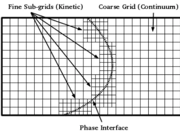
results are used to update the continuum data on the coarse grid.

Figure 1.7: Adaptive mesh refinement hones in on phase interface

The primary benefit of this approach is to balance efficiency and accuracy in the overall model. The use of the computationally expensive kinetic model is restricted to small domains near a phase interface or non-equilibrium section; areas where the kinetic model is theoretically more accurate. The computationally efficient continuum model is used everywhere else, in areas where continuum assumptions are valid. This approach also provides a nice way to implement macro-scale boundary conditions on a meso-scale model. The macro-scale forcings may be applied on the coarse continuum grid, and subsequently applied to the kinetic model by the mapping of continuum to kinetic variables.

The continuum-kinetic approach isn’t necessarily suited for every multiphase application. For instance, in some applications a purely continuum model may be sufficient for modeling purposes. In other applications, a kinetic model may be required for nearly the entire spatial domain, thus making the combined use of a continuum model excessive. This approach is best suited for a specific class of problems in which non-negligible meso-scale physical processes, occuring in a small portion of the spatial domain such as a phase interface, are critically linked to macro-scale physical phenomena.

1.9 Cold Spray

Cold Spray (CS) is a particle deposition process in which micron-scaled metal powder is sprayed onto a surface, gradually building up a new layer of material. CS was initially developed in the mid 1980s at the Siberian Division of the Russian Academy of Science as a coating technique [56]. Powder particles in sizes ranging from a few microns to tens of microns are transported through a spray gun by a carrier gas. Particle speeds typically reach just over a kilometer per second, though lesser speeds are sufficient for succesful spraying. Upon impact with the spraying surface, also called the substrate, particles undergo significant plastic deformation and a bonding mechanism that causes the particle to stick to the surface. An image of the crossection of an impacted particle is shown in figure 1.8.

Figure 1.8: Crossection of a copper particle embedded in an Al 7050 substrate [4]

sprayed material are closely related to the crystal structure of the ingoing powder. This enables a greater contol over resulting microstructural properties of sprayed materials.

Of interest in CS applications is the deposition efficiency, that is the mass fraction of powder that ultimately adheres to the substrate. High deposition efficiency is caused by a large percentage of impacting particles traveling above their respective critical velocities. Critical velocity is obviously closely connected to the physical mechanism responsible for bonding between particle and impact surface. Therefore, optimization of deposition efficiency requires an understanding of the bonding mechanisms.

The primary bonding mechanism in CS is a topic of much debate. Several mechanisms have been proposed: mechanical interlocking, localized melting at impact interface [61, 62], intimate contact [5, 63], and adiabatic shear instability [64, 65]. Mechanical interlocking occurs when the plastic deformation of the particle and substrate lead to an impact geometry that ’locks’ the particle to the substrate. Localized melting [61, 62] and rehardening of the surfaces at impact could explain bonding. However, evidence of melting is not always found in succesfully bonded particles [56]. Intimate contact [5, 63] is the theory that plastic deformation and the high pressure of impact lead to the disintegration of thin oxide films on the surface of the particle allowing the surfaces to come into close enough contact to form molecular bonds. Studies [64, 65] have linked the onset of adiabatic shear instability to the onset of succesful bonding. Adiabatic shear instability is a phenomenon within metal solids that occurs under very high strain rate. The instability is characterized by the metal exhibiting liquid-like behaviour at temperatures below the usual melting point. The appearance of a material ’jet’ (figure 1.9) flowing out from the interface is evidence of adiabatic shear instability occuring within the particle. Therefore, evidence of jetting is often viewed as a requirement for succesful bonding.

Figure 1.9: Jetting phenonmenon in CS single particle impact [5]

of the deposited layer was not uniform in space (figure 1.10). In particular, re-crystallization of grains was observed near impact interfaces; the grain sizes tended be larger at the cores and smaller near the edges of what once were individual particles. In [66], the microstructure of Titanium powder was analyzed under various pre-spray heat treatments. Pre-spray heat treatment was shown to have a noticeable effect on powder micostructure, and the implications of these effects on resulting material properties of sprayed deposits were noted. Several studies [67, 68, 69, 70, 71, 72] have analyzed the micro-structure of CS deposits of various materials. These studies confirm the lack of spatial homogeneity of microstructure in CS deposits.

1.9.1 Cold Spray Modeling

Having been discovered in the mid 90s, modeling of CS did not begin until the late 90s. Early CS models focused on elucidating the nature of bonding between particle and surface, thereby providing a prediction of the critical velocity. The purpose of these models was to reduce the cost of CS by offering insight that could improve the deposition efficiency of a spray. For this purpose alone, modeling efforts needed not attempt to predict microstuctural features. Phenomenological models of plasticity would therefore be sufficient to narrow the experimental search window for critical velocity. Furthermore, the modeling of a single particle impact by itself was usually enough to provide valuable insight on the physical processes behind particle adhesion. Even in more advanced models, like the one propsed in this thesis, the single particle impact is used as the basic element of CS modeling. Once a single particle impact model has been validated, multiple particle impacts can be simulated which may provide more insight on the material properties of deposits.

Figure 1.10: EBSD image of cold-sprayed Al 6061 crossection [6]

Laboratories to explore the nature of CS particle adhesion through the modeling of single particle impacts. The CTH code solves conservation laws in a two-step finite volume scheme. The first step approximates the solution to the conservation laws on a deformable Lagrangian mesh. The second step interpolates this data back to the original fixed Eulerian mesh. Therefore, overall the scheme can be viewed as Eulerian. Even the earliest CS modeling studies recognized that the large deformation and liquid-like flow in a CS impact would cause numerical problems. Their solution to the problem was to use an Eulerian description. In the CTH code, plasticity is introduced by an elastic-predictor plastic-corrector approach. If, after an elastic step, the predicted stress is outside the yield surface, the stress is projected back onto the yield surface in such a way as to most rapidly dissipate deviatoric stress. In these studies, either the Steinberg-Guinan-Lund [74] or Zerilli-Armstrong [75] plasticity models were employed.

out using the commerical software ABAQUS/Explicit. These studies used the numerical modeling results to validate the proposal of the adiabatic shear instability as the dominant bonding mechanism in CS. In [64], a sharp jump in plastic strain was observed near contact areas and associated with the onset of the adiabatic shear instability. The adiabatic shear instability has since been one of the predominant theories for CS particle adhesion. Other Lagrangian finite element models of CS include [76, 77].

The use of a Lagrangian mesh, while being ideal for precisely capturing material interfaces, is not ideal for the large deformations seen in CS. In particular, large deformation can lead to convoluted mesh distortion which must be dealt with in some way. Finite element modeling studies began to deal with this problem by using ALE [4, 61, 78, 79, 80] and fully Eulerian [81, 82] descriptions. These models used either ABAQUS or LS-DYNA commerical finite element software. In [78], it was shown that the sharp jump in plastic strain observed in [64] is no longer witnessed when using the ALE description as opposed to the Lagrangian description. This result casts some doubt on the adiabatic shear instability as the primary bonding mechanism.

The smoothened particle hydrodynamics (SPH) method has been used [83, 84, 85] as an alternative to finite element modeling to deal with the issues associated with Lagrangian mesh distortion in CS single particle impacts. The SPH method does not use any type of mesh. Rather, SPH uses representative particles to capture all relevant model physics. Conservation of mass, momentum, and energy are enforced by integration kernels which give weight only to the interaction of nearby particles. One issue with SPH is the clustering or thinning of particles that occurs when the material is compressed or stretched [83]. In [85], the SPH model was compared to both Lagrangian and Eulerian finite element models of CS impact. It was shown that the SPH model yields qualitatively similar results to the previously existing models.

based on consideration of dislocation motion, attained the closest results compared to experiment. While the dominant bonding mechanism is still an open question, more recently the focus of CS modeling has shifted to include the prediction of material properties of deposits. Obviously, the material properties of a deposit will depend on spray parameters like gas temperature, spray speed, and particle size. However, as discussed above, the microstructure of ingoing powder and its evolution during impact are non-negligible factors in the resulting material properties of sprayed deposits. Therefore, it seems inevitable that a model for predicting material properties must account for microstructure in some way. Since optimization of material properties is well-studied, both experimentally and numerically, with respect to the most obvious spray parameters, accounting for microstucture might be the most important contribution modeling can make to CS going forward. Indeed, consideration of microstructure introduces a much larger parameter space than before, making experimental optimization costly and time-consuming. Modeling that can reduce the experimental search space could be extremely valuable.

Unfortunately, modeling to this end has been limited in scope. In [89], the PTW model was used as a constitutive law in a Lagrangian finite element model of CS impact using ABAQUS/Explicit. The PTW model [88] is a physics-based plastic constitutive law developed for high strain rate loading conditions. The model is developed based on consideration of dislocation evolution, a meso-scopic physical process dependent on crystalline microstructure. Therefore, many of the model parameters can be determined by theory as opposed to experimental calibration. However, while being inspired by dislocation theory, the model itself does not explicitly capture microstructure. There are no additional state variables which track the evolution of microstructure. Thus, there is no way to predict the effects of differing microstructure in the initial powder.

Molecular dynamics models have been used to model thermal spray impacts [90, 91]. However, these models were limited to particle diameters of ones to tens of nanometers. Additionally, since particles are molten upon impact in thermal spray, an amorphous initial structure of particle and substrate is assumed. This assumption cannot be made for CS. It would also be computationally prohibitive to run an MD simulation for realistic sized CS powder particles. Nevertheless, MD can still be useful for understanding the physical processes in a CS impact. In [92], small scale impacts were simulated by MD to provide insight on adhesion and dislocation evolution in CS.

as the overall modeling objectives. As noted in previous studies, an Eulerian grid is adopted in order to avoid the potential issue of extreme mesh distortion encountered by Lagrangian studies. A crystal plasticity model is used to account for the effects of microstructural evolution. Microstructure may have an effect on this model in two ways: through the rotation of grains which cause the directions of dislocation motion to change, and through the blockage of dislocation motion at grain boundaries. Since the CP model is physics-based its parameters may be calibrated by small-scale MD simulations, like in [92], as opposed to experimental calibration. This feature is essential to the utility of the model in prediction of material properties. If it were necessary to experimentally calibrate the model, the original purpose of the model would be defeated.

A long term goal of the modeling project is to develop the capability to use both Johnson-Cook and CP models concurrently at different places in the simulation domain. This would use the approach illustrated in figure 1.7 in which the CP model would be employed in fine sub-grids focused on impact interface while the JC model would be used everywhere else. This approach would mitigate the computational expense from using the more complex CP model while still capturing the most important microstructural effects.

1.10 Outline

CHAPTER 2 Models

2.1 Linear Elasticity

A linear elastic model encompasses all constitutive models in which the dependence of the stress on the components of the deformation gradient (1.18) are linear. Typically, this means the stress is a linear function of strain and the strain a linear function of deformation. This type of model can be viewed as a linear approximation of the ’true’ relationships between stress and strain; strain and deformation. Therefore, linear models are only valid under specific physical conditions. First, a linear approximation of strain requires the deformation to be small. Second, a linear approximation of stress can mean one of two things: the loading of an elastic material must stay within the linear regime, or, in an elasto-plastic material, the onset of plastic deformation should come well before the non-linear regime. While these conditions are constrictive, if a simulation is expected to stay within these bounds, there is no reason not to use a linear model. Linear elastic models are simple to implement and are usually more computationally efficient than non-linear models.

The linear approximation of any physical strain tensor is equal to the Cauchy strain,

= 1

2(F+F

T_{)−I, (2.1)}

more commonly written in terms of the displacement

= 1

2(∇X~~u+∇X~~u). (2.2)

In a simple linear stress-strain model, stress can be defined as

or, in terms of displacements,

σij =λ ∂ux ∂X + ∂uy ∂Y + ∂uz ∂Z +µ ∂ui ∂Xj

+ ∂uj ∂Xi

, (2.4)

whereλandµare the Lamé coefficients. These coefficients are related to the speed of compressional and shear waves by

cp = s

λ+ 2µ

ρ , (2.5)

cs= r_µ

ρ. (2.6)

To utilize this constitutive law in a system of first order PDEs, the rate form of the equation is used

dσij

dt =λ

∂vx ∂X + ∂vy ∂Y + ∂vz ∂Z +µ ∂vi ∂Xj

+ ∂vj ∂Xi

. (2.7)

This type of model, in which the rate-form of the constitutive law is used as opposed to (2.3), is called a hypo-elastic model.

The rate-form equations (2.7) are combined with conservation of momentum equations (1.12) to form a closed system of equations. Since the stress (2.3) is symmetric, there are nine unique state variables in 3D (three velocity components, 6 stress components). Further, since small deformation is an assumption of the linear strain model (2.1), a Lagrangian formulation is employed, so the material derivative is simply

d dt →

∂

∂t (2.8)

Also, in a Lagrangian model, the density of a material point remains equal to the initial density

ρ(X, t) =~ ρ(X,~ 0) =ρ0(X)~ (2.9)

Taking everything into consideration, the full system can be written as

∂σxx

∂t −(λ+ 2µ) ∂vx

∂X −λ ∂vy

∂Y −λ ∂vz

∂Z = 0 (2.10)

∂σyy

∂t −λ ∂vx

∂X −(λ+ 2µ) ∂vy

∂Y −λ ∂vz

∂σzz

∂t −λ ∂vx

∂X −λ ∂vy

∂Y −(λ+ 2µ) ∂vz

∂Z = 0 (2.12)

∂σxy

∂t −µ ∂vy

∂X −µ ∂vx

∂Y = 0 (2.13)

∂σyz

∂t −µ ∂vz

∂Y −µ ∂vy

∂Z = 0 (2.14)

∂σzx

∂t −µ ∂vz

∂X −µ ∂vx

∂Z = 0 (2.15)

∂vx ∂t − 1 ρ0 ∂σxx ∂X − 1 ρ0 ∂σxy ∂Y − 1 ρ0 ∂σzx

∂Z = 0 (2.16)

∂vy ∂t − 1 ρ0 ∂σxy ∂X − 1 ρ0 ∂σyy ∂Y − 1 ρ0 ∂σyz

∂Z = 0 (2.17)

∂vz ∂t − 1 ρ0 ∂σzx ∂X − 1 ρ0 ∂σyz ∂Y − 1 ρ0 ∂σzz

∂Z = 0 (2.18)

2.1.1 Vector Form of System

In vector form, the equations can be written

∂q ∂t +A

∂q ∂X +B

∂q ∂Y +C

∂q

∂Z = 0 (2.19)

with

q =

σxx σyy σzz σxy σyz σzx vx vy vz T , (2.20) A=                          

0 0 0 0 0 0 −λ−2µ 0 0

0 0 0 0 0 0 −λ 0 0

0 0 0 0 0 0 −λ 0 0

0 0 0 0 0 0 0 −µ 0

0 0 0 0 0 0 0 0 0

0 0 0 0 0 0 0 0 −µ

−1/ρ0 0 0 0 0 0 0 0 0

0 0 0 −1/ρ0 0 0 0 0 0

0 0 0 0 0 −1/ρ0 0 0 0