Machine Learning for Stock Selection
Robert J. Yan
Computer Science Dept., The University of Western Ontario
Charles X. Ling
Computer Science Dept., The University of Western OntarioABSTRACT
In this paper, we propose a new method called Prototype Ranking (PR) designed for the stock selection problem. PR takes into account the huge size of real-world stock data and applies a modified competitive learning technique to predict the ranks of stocks. The primary target of PR is to select the top performing stocks among many ordinary stocks. PR is designed to perform the learning and testing in a noisy stocks sample set where the top performing stocks are usually the minority. The performance of PR is evaluated by a trading simulation of the real stock data. Each week the stocks with the highest predicted ranks are chosen to construct a portfolio. In the period of 1978-2004, PR’s portfolio earns a much higher average return as well as a higher risk-adjusted return than Cooper’s method, which shows that the PR method leads to a clear profit improvement.
Categories and Subject Descriptors
I.5 [PATTERN RECOGNITION]
General Terms
Algorithms
Keywords
Stock selection
1.
INTRODUCTION
Recently a considerable amount of work has been devoted to predicting stocks based on the machine learning techniques (e.g., [1;3;6]). These methods use a set of training samples to generate an approximation of the underlying function of data. Comparing with statistical methods, machine learning methods do not involve assumptions about sample independence or special distribution [7]. These assumptions may not always be met in the real world situations, which machine learning methods are designed to adapt.
In this paper, we investigate the issue of stock selection to form a portfolio with high return. In a real world trading environment, given a set of stocks, how can we select those “best” stocks? This task involves a ranking prediction of stocks and chooses the top ones to form the portfolio. The usual categorical prediction systems (i.e., The price/return trend prediction [3] that only predicts the direction of the price movement rather
than the expected price) are not appropriate for this task. For instance, we do not know how to select the 5-best stocks if the system predicts that 20 stocks will move upward.
Therefore, the task of stock selection needs a continuous prediction system. All the stock price/return prediction methods (i.e., linear regression) are continuous systems. However, they may still lead to unreliable results. When it comes to the individual stock prediction, the majority of previous methods (e.g.,[6]) select the model that achieves the maximum overall prediction accuracy (i.e., sum of squared deviations from actual outputs) for all stocks. However, in the case of stock selection, where the goal is to form a portfolio by those “best” stocks, we only care about the top performing stocks. Thus, the optimized model for all stocks may not be suitable for our task.
We propose a new method, namely Prototype Ranking (PR) that is based on the competitive learning [5]. PR is designed for the stock selection task rather than the individual stock prediction task. The overall prediction accuracy is no longer the primary objective during the model searching. Instead, PR tries to learn a network of prototypes, where the prototypes are the “super points” that represent a group of training samples nearby and the whole network can be considered as a model. This network has a better chance to distinguish the top performing stocks from ordinary stocks. PR is applied to samples of NYSE and AMEX individual stocks over the period 1978 to 2004. The experiments results show that PR is robust in short-term stock selection, and its performance is better than the traditional Cooper’s method of selection [2] after the transaction costs.
Section 2 defines the task of stock selection. Section 3 introduces the process of PR learning and testing. The experiments results are shown in section 4. A conclusion is given in section 0.
2.
DEFINING STOCK SELECTION TASK
In this section, we will discuss the formulation of stock selection task and its evaluation. We assume that trading days (when the market is open) are divided into “weeks” of five days labeled by the index t. The task of stock selection is to find n best performing stocks in the set of stocks tthat we choose for week t, given only information settavailable at the start of the week. In order to formulate the stock selection into a machine learning task we need to specify the following entities:
t is the training sample set of week t with N samples,
S(j t j, ) 1, , ;N t t
t
. Note that each sample in t
is associated with a specific week tprior to week t.
S( , ) ( ( , ),j t X j t RR j t ( , )) is a sample, where SRv is
the sample space and XRv1 is the predictor vector; RR
Permission to make digital or hard copies of all or part of this work for personal or classroom use is granted without fee provided that copies are not made or distributed for profit or commercial advantage and that copies bear this notice and the full citation on the first page. To copy otherwise, or republish, to post on servers or to redistribute to lists, requires prior specific permission and/or a fee.
KDD’07, August 12–15, 2007, San Jose, California, USA. Copyright 2007 ACM 978-1-59593-609-7/07/0008...$5.00.
is the stock real return and there exists a underlying function ( ( ))f Xt RR t( ) .
t is a separated testing sample set of week t with M
samples. t
S(j t, ) ( ( , ), X j t RR j t( , )) j1, , M
. As a typical machine learning process, a ranking function g that approximates f is learned from tby a specific algorithm. The rank of a testing sample j in t is then predicted by Rank j t g( , ) ( ( , ))X j t . After all the testing samples are assigned the predicted ranks, n stocks with highest/lowest ranks are selected to form a portfolio of week t. This process is repeated from the first testing week ts to the last testing week te. We can see that such stock selection task depends on two key decisions: How do we find the g?
What choice to make for the predictor vector? We will discuss how to use the competitive learning based method PR to find the ranking function g in section 3.1. For the predictor vector, we follow Cooper [2] in the choice of predictors. This will be discussed in section 4.1.
3.
PROTOTYPE RANKING
In this section, we discuss the algorithm of PR method consisting of a training process and a testing process. PR applies a modified competitive learning method to learn a ranking function g based on the training sample set and generates predicted ranks for testing samples. A quick review of traditional competitive learning is as follows: A competitive learning model (network) consists of H
prototypes
p p1, 2, , pH
. Prototypes could be thought ofas “super points” that represent a group of actual training samples around them in the input space Rv. Each prototype has
an associated reference vectorwRv. The general competitive
learning process can be described as follows:
1. Initialize the set by randomly choosing wifor each pi. 2. For each training sample SRv, calculate the distance
from S to each wi and choose one or several closest
prototypes (winners).
3. Adapt the reference vector of winners towards S:
( 1) ( ) ( )
wi t wi t S w i ε is the learning rate.
The competitive learning algorithms are widely used for making clustering analysis [5] and feature mapping [4].
3.1
PR Training
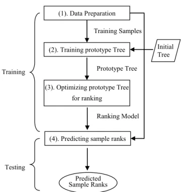
As shown in Figure 2, the PR training consists of the following three steps.
(1). Data Preparation. The raw stock data is converted into samples. For each week t, samples are divided into training samples and testing samples.
(2). Training prototype tree. The traditional competitive learning defines a mapping from the input data to a single
prototype network . A modified competitive learning algorithm is introduced in this paper, which maps the input data into multiple prototype networks arranged to a tree structure. We call these networks a prototype tree. Figure 1 shows an example of two-dimensional prototype tree with depth=3. In PR algorithm, an initial complete k-ary prototype tree of depth L is first created. Each node represents a fixed prototype in the predictor space Rv1, which is a subspace of the input sample space R .v Nodes
in the same depth are distributed uniformly to compose a network. The training process maps a training sample set
t
to a prototype tree. For each training sample ( , )S j t , PR searches its nearest prototypes (winners) on each tree level m. Those “winning” prototypes are then adapted to
( , )
S j t . Note that in PR, the searching of winners is performed in the predictor space Rv1instead of the entire sample space Rv , because the prediction task needs
patterns in Rv1 space. At the end of this step, we obtain a trained prototype tree. It reflects the patterns in the training samples.
(3). Optimizing the trained prototype tree into a ranking model for the minority samples. This step first prunes the redundant prototypes. If all the children of a prototype are similar to each other, they can be replaced by their parent prototype without information lost. Considering the majority of stocks are ordinary in a stock dataset, most prototypes in the tree must be trained to be “ordinary”. Such a tree tends to give “ordinary” predictions, which is meaningless to us. Pruning dramatically decreases the number of ordinary prototypes. After pruning, the tree has a better change to generate extreme predictions. However, single prediction is not what we need. To make the pruned tree predict relative relations among stocks, we assign each prototype an expected rank. By doing so, the pruned tree is converted into a ranking model. When it is used for prediction, testing samples that are close to prototypes with high expected ranks obtain high predicted ranking score.
3.2
PR Testing
The idea of PR testing is assigning each testing sample a predicted ranking score. Inside the ranking model obtained from the training, there are a number of prototypes with expected ranks distributed in theRv1. Since prototypes always represent
1
2
3
the nearby samples, the rank of a testing sample should be close to the ranks of its neighbour prototypes. Therefore, we may apply the kernel regression [10] to calculate the predicted rank of a testing sample. Those testing stocks with the highest/lowest predicted ranking scores are selected to form a portfolio. The real return of this portfolio is then evaluated as a measure to judge the performance of PR.
As a summary, PR method has several properties:
It has the ability to process the real-world stock dataset. To adapt to the new data, the model must be renewed every week. Considering the huge size of the real-world stock dataset, the batch methods that use all the available data to build a new model each week become impractical. Instead, PR adopts the on-line update mechanism. It uses only the latest data to update the old model.
PR method takes the properties of stock data into account. By applying the prototypes, PR can handle the data noise and data imbalance (i.e., there are many more samples belonging to one category than another).
PR method does not predict the individual stock return or price. The goal of PR is generating the ranking scores. The ranking score can be considered as the relative price/return and is more predictable than individual price/return [8].
4.
EXPERIMENTS
In this section, some empirical experiment results are discussed. In section 4.1, we first introduce the data used in the experiments. The procedure of the experiments as well as the measurement is discussed in section 4.2. In the following sections, the results of three experiments that we design to evaluate the PR methods are provided.
4.1
Data
The data come from the database of the center for Research in Security Prices (CRSP). We examine all samples of NYSE and AMEX individual stocks over the period 1962 (Dec.) to 2004 (Dec.). The stock universe we study is revised monthly. It consists of the 300 NYSE and AMEX stocks that have the largest market capitalization. In all 504 different stocks were chosen.
We convert the daily data into five-trading-day weekly data. In a given week, we omit any stock that has missing volume or price information for any of the previous ten days. Samples in the weekly data set have the same format:
( , ) ( ( , ), ( , ))
S j t X j t RR j t
where tis the index of week and j is the stock permanent number. The predictor vector ( , )X j t contains three predictors: Predictor 1 x(1,j,t’) = the return of stock j for the week t-1. Predictor 2 x(2,j,t’) = the return of stock j for the week t-2. Predictor 3 x(3,j,t’) = volume value ratio defined as 1 2
1 2
V V
V V
,
where V1, V2 are the values of the volume for stock j for weeks
t-1, t-2. Comparing with the volume ratio Cooper used, which is represented by 1 2
1
V V V
, our volume ratio leads to a more symmetric distribution of values.
4.2
Procedure
The PR method is evaluated in the time period from the first week of 1978 to the last week of 2004. We apply PR on tfor training a model and then make predictions for the stocks int.
To evaluate the performance of PR, we need to compare the predicted results with real results. As we mentioned in section 1, the overall criteria (i.e., the sum of square error) is not appropriate. The right thing we need to evaluate is the efficiency of the algorithm. That is, whether or not those stocks chosen by PR are “profitable”. Clearly, this could be evaluated by checking the real return of the chosen stocks, a portfolio.
In this paper we have used a simple portfolio formation scheme. Each week we form a neutral portfolio consisting of n stocks long and n stocks short. The long (short) stocks are those with highest (lowest) ranks. Each stock has equal weight (except when there are several stocks tied for last place, and then all those stocks are chosen with equal reduced weight). The average return of these portfolios over the testing time period, which is denoted by ARP , is what we study.
PR method aims to minimize the danger of data snooping. “Data snooping occurs when a given set of data is used more than once for purposes of inference or model selection” [9]. Therefore, the parameters of learning must be decided prior to the testing time period. In this experiment, PR searches the optimal values of its parameters in the time period from 1963 to 1977 and makes learning and testing in 1978-2004. Those optimal values of parameters are d=4,( ) 0.9t , k=9, s=4.5, and T=0.8.
We design two experiments for different evaluating purposes. Experiment 1 tests the predictability of the PR method. (1). Data Preparation
(2). Training prototype Tree Training Samples
(3). Optimizing prototype Tree for ranking
Prototype Tree
(4). Predicting sample ranks Ranking Model
Predicted Sample Ranks
Initial Tree
Testing Training
Experiment 2 compares PR method with Cooper’s method both before and after the transaction costs. In these experiments, we divide the testing period into two (1978 - 1993 and 1994 – 2004), because 1978-1993 was the one Cooper used for his tests so we can obtain a direct comparison.
4.3
Experiment 1
The predictability of PR can be evaluated by comparing the returns of different portfolios it constructs in the same time period. Given a week t, two portfolios P1, P2 are constructed.
P1 has 2n1stocks and P2 has 2n2 stocks. We denote the expected return and the real return of a portfolio P in week t
as RP( )P and RP( )P respectively. Naturally, if a portfolio performs as it is predicted, the algorithm that generates the portfolio is considered to be with predictability. The condition of predictability can be defined as:
Assume that an algorithm predicts P1 is better P2, which means thatRP( 1)P RP( 2)P . If
(RP( 1)P RP( 2))P (RP( 1)P RP( 2)),P
then this algorithm has the predictability in week t. However, PR does not really calculate the expect return of a portfolio. PR always chooses the stock with the highest (lowest) rank and the chosen stock always has the highest expected return in the set of remaining stocks. The more stocks involved in a portfolio, the lower its expected return. Therefore we may change the condition of predictability to:
If (n1n2)(RP( 1)P RP( 2))P , then PR has the predictability in week t.
Similarly, the condition of predictability in a certain time period is defined as follows.
If (n1n2)(ARP( 1)P ARP( 2))P , then PR has the predictability in this time period.
However, the above condition only works in the pure dataset with no noise. Given a real-world stock dataset, PR generates two portfolios P1 with n1 stocks and P2 with n2stocks. If
1
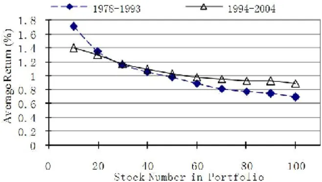
nand n2are too close (i.e., n15 andn26), even if PR has a certain level of predictability, the above condition may still be violated because of the heavy noise in the training samples. To correctly reflect PR’s predictability under the noisy environment, the difference betweenn1and n2should be larger enough to tolerate the noise. We always set thatn2 n1 5. In this experiment, for both time periods 1978-1993 and 1994-2004, PR generates ten portfolios with different stock numbers 2n ( n 5 ,i i1, ,10 ). We compare these portfolios and present the results in Figure 3. For each time period, the predictability condition has been tested by 9 cases. In all the cases, the condition is satisfied. In both given periods, the average return of the portfolio increases steadily as n decreases from 50. In addition, we calculate the return difference db/w
between the return of the expected best portfolio and the return of the expected worst portfolio. db/w represents the level of
predictability in a way.
/ ( )P ( )P
b w
d RP i RP j
where Piargmax{RP( )}P and Pjargmin{RP( )}P . We may rewrite the equation as follows.
/ ( (P 5)) ( (P 50))
b w
d RP n RP n
In 1978-1993, db/w is 1.01% and in 1994-2004, db/w is 0.7%.
They are both significant changes. All these results show strong evidences of the predictability of PR over 1978-1993 and 1994-2004.
4.4
Experiment 2
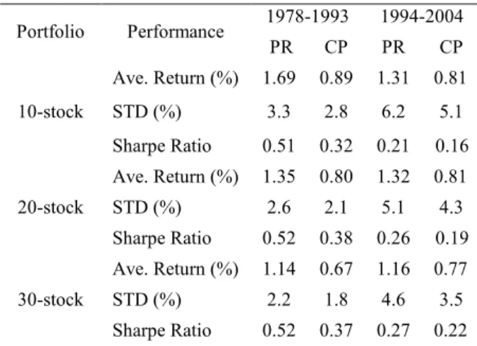
In this paper, we focus on the short-term stock selection based on only historical return and volume information. Cooper [2] investigated the same problem and proposed a method (CP). In the learning phase, Cooper first, for each predictor, divides into deciles the historical distribution of predictor values. Using the decile boundary values, the three-dimensional predictor space is partitioned into 1000 cells, with each cell assigning an average one-week return of all stocks in it. In the testing phase, the average return of a cell can be used as the predicted return of testing samples belonging to this cell. CP has no machine learning techniques involved. The comparison between PR and CP will show us whether the stock selection task benefits from applying some machine learning techniques. We apply both PR and CP to the same stock data set using the same procedure discussed in section 4.2. For each week from 1978 to 2004, each method forms three weekly portfolios with 10, 20, 30 stocks respectively. Table 1 reports their performances in 1978-1993 and 1994-2004. In all cases, the PR earns higher Ave. return compared with CP. The average margin of three PR returns over three CP returns in the 1978-1993 is 76.3% and in 1994-2004, it is 58.4%. We also compare the risk-adjusted portfolio performance, which is usually measured by the Sharpe Ratio (retun/std.). Table 1 shows that in this case PR also outperforms CP. For example, the Sharpe Ratios of three PR portfolio over 1978-1993 are 0.51, 0.52, and 0.52 respectively. In contrast, the Sharpe Ratio of CP portfolios are 0.32, 0.38, and 0.37 over the same time period, respectively. The comparison in 1994-2004 shows the similar results.
The above experiment compares the predictability of PR and CP and shows that PR generates more accurate and stable predictions. We also evaluate whether PR’s predictions are more profitable compared to CP’s predictions under the transaction costs. The final investment value (FIV) of the portfolios under the transaction costs is used as the measure. Although estimating the real transaction costs of each trade is difficult, it is
reasonable to suppose that the costs for CP and PR would have been similar. For technical convenience, we follow Cooper [2] in setting the round-trip cost levels to evaluate the after-cost performance for both methods:
0.25%; 1 (low transaction costs) Transaction costs 0.5%; 2 (medium transaction costs) 0.75%; 3 (high transaction costs)
l
l
c l
l
Table 1. The Performance Comparison: PR v.s. CP
Portfolio Performance 1978-1993 1994-2004 PR CP PR CP 10-stock
Ave. Return (%) 1.69 0.89 1.31 0.81 STD (%) 3.3 2.8 6.2 5.1 Sharpe Ratio 0.51 0.32 0.21 0.16 20-stock
Ave. Return (%) 1.35 0.80 1.32 0.81 STD (%) 2.6 2.1 5.1 4.3 Sharpe Ratio 0.52 0.38 0.26 0.19 30-stock
Ave. Return (%) 1.14 0.67 1.16 0.77 STD (%) 2.2 1.8 4.6 3.5 Sharpe Ratio 0.52 0.37 0.27 0.22 We compare the 10-stock portfolios of PR and CP, which represent their best profitability. Considering that the investing is a continuous process, we do not split the testing period. Therefore we calculate the FIV of the portfolios in 2004 (Assume that investors start off with $1 in 1978 and reinvest the portfolio income every week) under different transaction costs. These results are shown in Table 2.
Table 2. The FIV Comparison: PR v.s. CP
Transaction Costs FIV of PR (2004) ($)
FIV of CP (2004) ($)
Low 6E5 256.5
Medium 717.7 0.22
High 1.43 0
For both methods, the profit drops dramatically as the transaction costs increase from 0.25% to 0.75%. Under the same costs level, PR always outperforms CP. At the low cost level, the FIV of PR and CP in 2004 are $ 6E5 and $256, respectively. In the cases of medium and high transaction costs, PR portfolios are still profitable. The FIVs of PR are $717.7 (medium) and $1.43 (high). In contrast, the profit of CP portfolios has disappeared under medium or high transaction costs. As we expected, PR survives a higher level of costs relative to CP and shows better profitability.
5.
CONCLUSION
This paper proposed a machine learning method called Prototype Ranking (PR) for short-term stock prediction. The goal of the PR method is to select n best performing stocks from a stock set based on the ranking function g learned in the
historical stock data. PR applies a modified competitive learning technique, which is designed for discovering models under the noisy and imbalanced environment. In the testing phase, each testing sample is assigned a predicted ranking score and the stocks with the highest/lowest ranks are selected to form a portfolio. The experimental results show strong evidences of the predictability of PR. In addition, PR outperforms CP, which is a non-machine-learning method. This shows the advantage of applying machine learning in the short-term stock prediction. This work can be further improved in two directions. First, given current predictors, we may apply boosting techniques to improve the accuracy. Second, in the paper we only apply the short-term predicting. It is possible to combine the short-term predicting with the long-term predicting for the stock selection.
6.
ACKNOWLEDGMENTS
We appreciate the access to the CRSP database provided by the University of Western Ontario via the WRDS system.
REFERENCES
[1] Avramov,D., and Chordia,T. (2006), Predicting stock returns, Journal of Financial Economics 82, 387-415. [2] Cooper,M. (1999), Filter rules based on price and volume
in individual security overreaction, Review of Financial Studies 12, 901-935.
[3] Edwards,R.D. and Magee,J., Technical Analysis of Stock Trends (Amacom Books, 1997).
[4] Fritzke,B. (1994), Growing Cell Structures - A Self-Organizing Network for Unsupervised and Supervised Learning, Neural Networks 7, 1441-1460.
[5] Fritzke,B. Some competitive learning methods. 1997. [6] Hamid,S.A., and Iqbal,Z. (2004), Using neural networks
for forecasting volatility of S&P 500 Index futures prices, Journal of Business Research 57, 1116-1125.
[7] Hastie,T., Tibshirani,R., and Friedman,J.H., The Elements of Statistical Learning (Springer, 2003).
[8] Hellstrom,T. (2001), Optimizing the Sharpe Ratio for a Rank Based trading System, EPIA 2001, LNAI 2258 130-141.
[9] Sullivan,R., Timmermann,A., and White,H. (1999), Data-Snooping, technical trading rule performance, and the boostrap, The journal of Finance 54 1647-1691. [10] Wolberg,J.R., Expert trading systems : modeling
financial markets with kernel regression (; Wiley, New York 2000).