Development of the US3D Code for Advanced
Compressible and Reacting Flow Simulations
Graham V. Candler
∗, Heath B. Johnson
†, Ioannis Nompelis
‡,
Pramod K. Subbareddy,
‡Travis W. Drayna
§, Vladimyr Gidzak
¶,
Aerospace Engineering and Mechanics, University of Minnesota, Minneapolis, MNMichael D. Barnhardt
kERC Inc. at NASA Ames Research Center, Moffett Field, CA
Aerothermodynamics and hypersonic flows involve complex multi-disciplinary physics, including finite-rate gas-phase kinetics, finite-rate internal energy relaxation, gas-surface interactions with finite-rate oxidation and sublimation, transition to turbulence, large-scale unsteadiness, shock-boundary layer interactions, fluid-structure interactions, and thermal protection system ablation and thermal response. Many of the flows have a large range of length and time scales, requiring large computational grids, implicit time integration, and large solution run times. The University of Minnesota / NASA US3D code was designed for the simulation of these complex, highly-coupled flows. It has many of the features of NASA’s well-established DPLR code, but uses unstructured grids and has many ad-vanced numerical capabilities and physical models for multi-physics problems. The main capabilities of the code are described, the physical modeling approaches are discussed, the different types of numerical flux functions and time integration approaches are outlined, and the parallelization strategy is overviewed. Comparisons between US3D and the NASA DPLR code are presented, along with several advanced simulations to illustrate some novel features of the code.
I.
Introduction
The University of Minnesota, in collaboration with the NASA Ames Research Center, has developed a computational fluid dynamics code, US3D, for the simulation of compressible and reacting flows.4, 5 Through
this effort, the US3D software package now possesses a broad base of modeling capabilities and powerful analytical tools that make it well-suited to large-scale simulations of a broad range of flows. This paper documents the capabilities of the code, shows validation results, and illustrates its use on a variety of high-speed flow simulations. Several key code design decisions are discussed, and the codes parallel scaling is demonstrated.
The US3D code is designed to be the next-generation version of the well-established NASA DPLR (data-parallel line-relaxation) code.6 The main difference is that US3D uses unstructured grids composed of
∗Russell J. Penrose and McKnight Presidential Professor and Fellow AIAA †Senior Research Associate, Member AIAA
‡Research Associate, Member AIAA
§Currently, Principal Engineer, GoHypersonic Inc., Member AIAA ¶Post-Doctoral Research Associate, Member AIAA
kAerospace Engineer, Senior Member AIAA
tetrahedra, prisms, pyramids and hexahedra, which has important advantages for certain classes of prob-lems, particularly those involving complex geometries or which require localized resolution of the flow field. However, many aerothermodynamics problems require the use of hexahedral grids to provide optimal accu-racy. For such problems, the unstructured formulation is beneficial because it promotes topological flexibility in the underlying block structure of the mesh. With no limitation on the number of grid blocks in US3D, the burden of complex grid generation is diminished.
The primary solution approach uses the same implicit data-parallel line-relaxation method as DPLR, along with similar forms of upwind numerical flux functions. DPLR’s most commonly used physical models have also been replicated in US3D. It can be run with finite-rate internal energy relaxation and chemical kinetics, it has several popular turbulence models, and it has many standard surface boundary condition models. Like DPLR, kinetic mechanisms, transport properties and other model parameters are easily speci-fied through an extensible set of input databases. Indeed, US3D supports direct use of the DPLR database if the user chooses. And yet, US3D has a number of distinct capabilities beyond those available in DPLR.
Perhaps the most powerful innovation is the introduction of an application programming interface (API) which enables users to modify the code’s execution without requiring manipulation of the core source code itself. Most aspects of execution can be tapped by a user in this way: code input or module definition, initialization, numerical integration, flux functions, boundary conditions, even the underlying equations themselves. In this way, users are not limited to US3Ds core capabilities and can tailor the code to their specific application.
Another unique capability of US3D is the ability to run with numerical flux functions of different levels of accuracy and dissipation. The standard approach is to use MUSCL-limited, second-order upwind fluxes, but these can be switched to unbiased second-, fourth- and sixth-order numerical fluxes with various choices of shock detectors and added dissipation to maintain stability. Along with these more accurate fluxes, time integration can be performed with different levels of accuracy to support time-accurate unsteady simulations, wall-modeled large-eddy simulations, and direct numerical simulations. This flexibility in numerical methods is useful for investigating the effects of numerical dissipation and accuracy on complex unsteady flows.
For some applications that require a large number of chemical species, the standard DPLR approach of coupled species mass equations is demanding because its cost scales with the number of species squared. Recently, an implicit method was developed that decouples the mass, momentum, and energy conservation equations from the species mass, internal energy, and turbulence transport equations. This approach has been shown to significantly reduce the computational costs and memory requirements of certain classes of problem. This approach is implemented in US3D for steady-state problems, and an unsteady formulation is in development.
US3D permits multiple, independent grids to be used so that the gas dynamics can be solved on one grid, and material response can be solved on another, for example. This makes the code simple to use for conjugate heat transfer problems and other simulations that require the solution of multiple sets of governing equations in different regions. US3D is also able to perform time-accurate dynamic simulations involving grid deformation and grid motion. This approach has been used to study the dynamic stability of capsules, for example. If the grid motion is coupled to the multiple-grid solution capability, it is straight-forward to perform thermal response and ablative shape-change problems with US3D. Several additional capabilities are under development and testing.
At the present state of development, the US3D code represents a unique simulation tool for a wide range of aerothermodynamics and hypersonic flow simulations. In the following, we discuss the design of the code, outline the methods used, the physical models implemented within US3D, compare with benchmark DPLR data, present scaling results, and illustrate the use of US3D on several example problems.
II.
Physical Models
II.A. Thermo-chemical ModelsUS3D was originally developed as a CFD code for aerothermal and high-temperature reacting flow simu-lations; it solves species mass conservation equations forns species, momentum, total energy, and internal
(vibration and electronic) energy. The chemical species react with one another according to the law of mass action, and the internal energy relaxes toward the translational-rotational energy according to the Landau-Teller model. This formulation is the standard approach for high-temperature nonequilibrium flows.1–3
The chemical kinetics models can be specified using previously-developed “gas” files, or users can build their own. Reactions are specified according to type and the names of the reactants and products; the appropriate governing temperature for the reaction may also be set. Reaction rates are given in Arrhenius form, and the equilibrium constants are computed from Gibbs free energy minimization using the NASA Lewis CEA database.7, 8 US3D forms the chemical source term for the given arbitrary set of reactions,
along with the analytic form of the Jacobian of the source terms for use with implicit time integration. The Jacobian formulation has been verified through comparisons with numerical derivatives.
In the US3D formulation, the translational and rotational energy of the gas mixture is governed by a single temperature,T. The internal energy can be modeled in several ways: (1) it can be neglected entirely; (2) it can be represented with a simple harmonic oscillator model for vibrational energy with a single vibrational temperature, Tv; (3) it can be computed from the enthalpy fits from the CEA database, which inherently
includes anharmonic vibrational energy and electronic energy, yielding a vibrational-electronic temperature; or (4) it can be equilibrated with the translational-rotational energy using the CEA data. The numerical flux functions are formulated to correctly account for the different representations of the internal energy. By default, Millikan-White relaxation times9 are used for the internal energy relaxation rate, but the user can
specify exceptions to this model. Also, the Park high-temperature limit10 is used to prevent the relaxation
from becoming faster than the collision time. At very high temperature where electronic energy dominates the internal energy, this becomes the effective relaxation time.
Within US3D, various transport property and mass diffusion models may be specified. These include Blottner fits and Gupta collision integral representations for the species viscosity;11 thermal conductivity
is computed using an Eucken relation. The mixture transport properties are then computed with a choice of Wilke12 or Armaly-Sutton13 mixing rules. The mass diffusion fluxes are modeled with simple Fickian
diffusion or several variants of the Ramshaw-Chang self-consistent effective binary diffusion model14, 15using
Gupta-Yos collision integral data.11 The user may also specify transport property models if required.
US3D also includes the first-order correction to the thermal equation of state to account for high-pressure effects. This excluded-volume formulation makes the pressure a non-linear function of density, which must be included in the computation of the fluxes, speed of sound, and enthalpy. It has been shown to be effective in representing the high-pressure effects in hypersonic blow-down wind tunnels, for example.16
The US3D code is being used for low Mach number problems for which a perfect gas model is accurate and the number of conservation equations to be solved is fixed. In this case, the generality of the US3D thermo-chemical model increases the cost of a computation relative to a code designed for a perfect gas. Therefore, compiler directives have been included in US3D so that a perfect-gas version of the code can be compiled; this results in substantial improvement in computational time due to improved compiler optimization and reduced use of conditionals.
II.B. Boundary Conditions
In high-temperature aerothermal problems, the gas-surface boundary condition may be extremely complex and is usually specific to the surface material properties. Thus, there are a very large number of possible combinations of surface boundary condition models. These can involve: (1) isothermal, adiabatic, radiative equilibrium, or some other form of surface energy balance; (2) non-catalytic, partially catalytic, or finite-rate gas-surface chemical kinetics for the thermo-chemical state; (3) blowing or ablation species formation,
including surface motion or recession; (4) rarefaction effects resulting in velocity and energy slip at the surface; (5) general mass and energy balance coupled to the in-depth thermal response of the thermal protection system material.
US3D provide built-in boundary conditions for the simple variants of the above list; for specific appli-cations, the user may implement boundary conditions through the user-specified API. There is a growing library of advanced boundary conditions and a near-future version of US3D will have a unified framework for the implementation of arbitrary boundary conditions.
US3D also includes a variety of standard characteristics-based subsonic and supersonic flow-through boundary conditions, as well as symmetry boundary conditions.
II.C. Turbulence Models
Reynolds-averaged Navier-Stokes (RANS) turbulence modeling for highly compressible reacting flows remains a black art, with model performance highly dependent on the particular application; US3D has several of the most popular turbulence models – these include the Spalart-Allmaras model17 with the Catris-Aupoix
compressibility correction18 (the SA-Catris model in the NASA Langley turbulence modeling
nomencla-ture19), the recent SA-neg model,20 and the Menter SST (SST-V) model.21 For hybrid RANS / large-eddy
simulations (LES), US3D has several approaches, including DES97,22 DDES,23 and IDDES;24 all of which
are based on the SA-Catris model. When running in pure LES mode, the Smagorinsky25 and Vreman26 subgrid-scale models may also be used. For legacy reasons, the Baldwin-Lomax model27is also implemented
in US3D.
The RANS models may be run in fully turbulent mode, or the SA-Catris model may be tripped at discrete locations. In the latter case, either the default SA trip model may be used, or the user may specify a trip model that is designed to mimic physical boundary-layer trip elements. (With hypersonic boundary layers, it may be difficult to activate the SA turbulence model and the default natural trip usually does not provide adequate forcing to the model.)
II.D. Thermal Response, Conjugate Heat Transfer, and Shape-Change
Many hypersonic and aerothermal problems include coupling between the fluid motion, aerothermal effects, surface boundary conditions, and the vehicle thermal response. In cases with ablation, the surface may recess, causing geometric shape change. US3D may be run in a mode to model all these effects in a fully-coupled fashion.
US3D treats the computational grid as a grid object, which permits specific operations to be performed on the object (for example, partitioning of the grid object). Thus, within US3D it is possible to operate on more than one grid object – in this case, there is a fluid grid and a solid grid, both of which are partitioned across the parallel computer. These grids are assumed to be face-matched at their interface. A simple point implicit relaxation method is used to solve the thermal response of the solid represented by the solid grid. Data are passed between the two grids to synchronize the interface boundary condition.
The coupled fluid-solid response can be run in a fully time accurate mode, or the usual large discrepancy between the fluid and solid time scales can be exploited by running in quasi-steady mode. Here, the steady-state fluid heat flux if passed to the solid, which is then integrated over a relevant time scale. The near-surface solid temperature is passed to the fluid, which is then re-converged, and the cycle is repeated. This quasi-steady approach is valid and stable, provided that the solid integration time is small relative to the rate of change of the surface properties (heat flux in particular). If solid shape change is included, the fluid and solid grids are moved once prior to re-convergence of the fluid, and the grid motion terms are included in the flux and fluid update calculations.
II.E. Bow Shock / Grid Alignment
It is well known in the aerothermodynamics literature that CFD solution accuracy is greatly improved if the grid is aligned with the bow shock wave.28, 29 If a strong shock crosses the grid obliquely, it generates spurious post-shock vorticity and entropy which persist in the downstream flow. US3D, like the LAURA31
and DPLR codes, has utilities to improve grid alignment; this requires the generation of grids that have line-solve lines that run from the vehicle surface to the free-stream boundary. Typically, a solution is run on an initial grid until convergence, then the shock “tailoring” or alignment routine is called – this detects the location of the bow shock and scales the grid so that the shock is located at a fixed number of elements along the line from the body surface. The solution is then re-converged, and shock tailoring may be performed a second time if required. A more general approach is under development that uses the grid deformation capabilities of US3D to gradually deform the grid until it is shock-aligned.
II.F. Lagrangian Particle Tracking
A recent addition to the US3D code is the ability to solve for the motion of particles within a fluid domain.30
This capability was added for the solution of the Filtered Mass Density Function (FMDF) stochastic dif-ferential equations for turbulent combustion simulations. It can also be used for multi-phase flows, or even potentially for hybrid continuum / Direct Simulation Monte Carlo (DMSC) computations. The approach for Lagrangian particle tracking involves creating a linked list of particles that are present within each grid element, and then integrating these particles on their trajectories through the grid element. When a particle crosses into a new element, it is deleted from the old element list and added to the new element list. Parti-cles may be generated or deleted to maintain a reasonable or desired population per element. The overhead associated with particle tracking is typically about 30% for 50 particles per cell, relative to a third-order Runge-Kutta explicit time integration step.
III.
Numerical Methods
The US3D code was initially developed to be an unstructured grid version of the multi-block structured grid code, DPLR. This is a finite-volume code, with data stored a element centroids and fluxes evaluated at element faces. US3D has many of the same numerical methods as the DPLR code, but modified for unstructured grid framework. Over the years, this basic set of numerical methods has been greatly extended to include novel high-order, low-dissipation numerical methods and other features. In this section, the methods implemented within US3D are summarized. For additional information and mathematical details, the interested reader is referred to several recent papers.32, 33
III.A. Numerical Flux Functions
For steady-state laminar and RANS turbulent simulations, second-order accurate upwind methods are the default approach for representing the numerical flux in compressible flows. US3D uses a modified form of the Steger-Warming flux-vector splitting approach;34, 35 here the convective flux is written as the product of the
flux Jacobian matrix,A, and the vector of conserved variables,U, evaluated at the element face of interest. The matrix A is split into left- and right-moving components based on the sign of its eigenvalues. Then, left- and right-moving fluxes can be constructed from the split Jacobian matrices. In the original Steger-Warming approach, both the split Jacobians andU were evaluated with upwind variables. With the present approach, both the left and right Jacobians are evaluated with symmetric unbiased data across the face, which drastically reduces the level of numerical dissipation (particularly in regions of shear). This approach produces a numerical flux that is similar to the Roe flux,36 and has been shown to produce similar results
for hypersonic flows. When there is a strong shock wave or other discontinuity across a face, the unbiased averaging of the split Jacobian matrices does not provide sufficient dissipation; in this case, the Jacobians are upwind-biased based on a smooth pressure sensor. The conserved variable vector,U, is evaluated with
upwind data. This is done with the MUSCL approach,37 in which the extrapolated data are limited to
produce a total variation diminishing flux. For high-temperature applications, the species densities, velocity, pressure, and specific internal energy are extrapolated and limited, and then U is computed from these values. This reduces spurious pressure variations in boundary layers, for example.
For applications with very rapid reactions, limiting the species densities in an equation-by-equation fashion can result in poor results due to elemental non-conservation and aphysical species overshoots and undershoots. Fixing this problem is a topic of current research.
The conventional second-order (or potentially third-order with the QUICK scheme) accurate, upwind-biased approach is not adequate for most unsteady flows because of the inherent dissipation. An alternative approach is to use an unbiased numerical flux function, and then to add dissipation if needed to control error. US3D uses a kinetic energy consistent (KEC) flux that was designed to produce a numerical flux that is discretely consistent with the compressible kinetic energy transport equation.38 Such a numerical flux is
inherently more stable than one that does not enforce bounds on the kinetic energy variation. Dissipation is added to this flux function using a discontinuity sensor (for example, that of Ducros39), and then adding
a scaled dissipative flux from the modified Steger-Warming flux discussed above.
III.B. Higher-Order Accuracy
The KEC flux approach has been extended to fourth and sixth order accuracy through the use of additional cell-centered gradient information. US3D uses weighted least-squares to evaluate the gradients of the flow variables for the viscous flux calculation. If these gradients (computed at cell centers using a cloud of neighboring data) are used along with the element-centered data, a fourth-order flux can be constructed. This assumes smooth variation of the variables on a smoothly-varying hexahedral-element grid. Using gradients at neighboring elements on a hexahedral grid, it is possible to extend the fluxes to sixth-order accuracy. This theoretical result has been demonstrated on test problems.40
III.C. Viscous Fluxes
As mentioned above, US3D uses weight least-squares to fit a hyperplane through a cloud of data; then element face gradients are computed using a deferred correction approach.41 This improves the approximation of
the gradients in the regions of high cell-aspect ratio (highly stretched) grid elements, and is consistent with optimal gradient formulations. This approach is different than the DPLR code, and may account for some differences between the codes – objectively, the present approach will be more accurate on non-ideal grids, and will revert to the non-corrected result on ideal grids.
III.D. Time Integration Methods
The DPLR code was named for the implicit data-parallel line-relaxation (DPLR) method that was a key innovation in its development. The DPLR method solves the implicit linearized system of equations by constructing a block tridiagonal problem along identified lines, while relaxing contributions from off-line terms. Excellent convergence to steady-state is obtained when the line-solve direction is consistent with the direction of the strongest physical coupling. For example, for the flow over a planetary entry capsule the wall-normal direction has the largest gradients, and the smallest grid spacing – due to the resolution requirements of the boundary-layer flow. If the line-solve direction is taken as the wall-normal direction, the dominant physics is consistent with the numerics, and excellent convergence is obtained. Another part of the success of the DPLR method is due to the use of modified Steger-Warming flux-vector splitting, because the exact flux Jacobians can be used to form the linearized implicit operator.
US3D is an unstructured grid code, and it is not possible to form lines along a constant ordered grid index. Instead, solution lines must be constructed by connecting faces and elements where possible. In US3D, the user specifies a set of boundary faces and maximum line length, and the code starts at each face on the boundary and grows lines using connectivity information. Lines are formed until the next adjoining
element is a pyramid or tetrahedron, the element is already part of a different line-solve line, or the maximum line length has been reached. Typically, lines are grown starting from wall boundaries, but in some cases it may be beneficial to grow lines from other boundaries. Regions of the grid that are not included in line-solve lines are computed with a point-implicit method.
For unsteady problems, line relaxation gives poor results because the assumed coupling direction biases the solution and is only first-order accurate (although it can be extended to second-order). Therefore, US3D has several higher-order explicit and implicit time-integration methods. With hybrid RANS/LES, a particularly useful approach is second-order accurate implicit point-relaxation, which is typically run at CFL numbers of order 100 (100 times the theoretical maximum explicit time step). This results in approximate time accuracy in the near-wall elements, but very good accuracy in the unsteady region where the grid elements are larger. Such an approach makes hybrid RANS/LES feasible for many problems.
US3D also has higher-order explicit methods that are typically used for non-wall-bounded LES and direct numerical simulations of turbulent flows.
III.E. Decoupled Implicit Method
The implicit DPLR method that is central to the US3D code solves the governing equations as a fully-coupled system of equations. This results in a set of block-tridiagonal problems that are solved along lines, as discussed above. The cost of the solution varies with the square of the number of equations, ne, being
solved, so large numbers of chemical species incur a very large computational cost. In addition, to represent the system of equations, sevenne×nematrices must be stored for every grid element.
Recently, a decoupled approach was developed, in which the solution is separated into two sequential parts, each solved with a modified version of the DPLR method.42 First, the equations for total mass,
momentum, and energy are solved, and then the species mass, internal energy, turbulence equations are solved. With minor modifications to the implicit system, the cost of the second phase of the solution can be significantly reduced, making its cost essentially linear in the number of equations. (However, the cost of evaluating the chemical source term is inherently quadratic in ns.) Furthermore, the memory costs are
significantly reduced, as only a single large Jacobian matrix must be stored at each grid element. This decoupled method is particularly effective when the reaction rates are not very fast relative to the fluid motion rate (moderate to low Damkohler number). For a chemical kinetics model with 20 species, this approach is approximately 3 times faster than the fully-coupled method, with a similar reduction in memory requirements. This method is implemented in the US3D code as an optional solution mode.
III.F. Sensitivity Variables and Newton-like Convergence
Several studies have been conducted with US3D to optimize hypersonic flight vehicles; here the objective function and its gradients must be computed to drive the optimizer. The standard approach is to linearize the governing equations and the boundary conditions and solve the resulting linear system for the sensitivity variables – the gradient of the solution with respect to the design variables (for example, parameters that describe the geometry). However, it was found that for hypersonic flow problems dominated by highly non-linear processes, this non-linearization often produces the wrong answer, and can even result in the wrong sign of the objective function gradient. Therefore, a fully non-linear sensitivity variable solution was developed that uses much of the existing US3D infrastructure.43 This method produces Newton-like convergence to
steady state (convergence in about 20 iterations).
The Newton-like convergence of the sensitivity solver can be exploited for other purposes besides opti-mization. For example, if an angle of attack sweep is required for a particular geometry, the first condition can be computed running in conventional DPLR mode; then the free-stream flow angle is changed and the sensitivity solver is used to rapidly re-converge the solution to the new angle of attack. This results in significant savings relative to restarting and running in conventional DPLR mode.
III.G. Unsteady Grid Motion
A novel feature of US3D is the ability to perform dynamic grid motion simulations, while maintaining grid quality, even after large levels of grid deformation. It is not possible to provide full mathematical details of the approach here, but conceptually the grid is constrained to follow rigid-body motion near moving solid surfaces to preserve the near-wall grid spacing. In non-near-wall regions, the grid deforms through a combination of rigid-body translation, rigid-body rotation, and compression.44 The grid deformation is
enforced at grid nodes, not at element centroids, which is crucial for maintaining grid quality and preventing high-frequency instabilities in the grid.
IV.
Parallelization Approach
US3D was initially designed to scale well on large numbers of processors for large grids, however what constitutes “large” is a rapidly changing quantity. Currently, US3D has been shown to scale well to 20,000 cores for half-billion hexahedral element grids. Work is continuing to permit multi-billion element grids to be simulated on larger partitions. In this section, we briefly discuss the approach used to parallelize the key phases of operation of the US3D code. We consider operation on a conventional distributed memory computer cluster composed of compute nodes, each of which has the same number of multi-core processors.
IV.A. Grid Partitioning
US3D uses the ParMETIS parallel graph partitioning library45 to partition the grid as the first step in
running a simulation. The grid is read from a single HDF5 file, either by core 0, which distributes the data across the machine, or by each core in parallel, if supported by the filesystem. Next, implicit solution lines are constructed by starting at a specified boundary face and finding connected elements from the connectivity information, as described above. This is a distributed process because the next element in any given line may be owned by any other core; data are passed between cores at each step in the line-finding process. The connectivity graph associated with the lines is then collapsed to a single graph node, and weighted to reflect the number of elements within the line. This modified graph is then passed to ParMETIS and the grid is partitioned. Finally, the grid and connectivity data associated with each partition are collected onto the corresponding core.
A crucial feature of the US3D partitioning is that the data required for the block-tridiagonal solution are always on the same partition. Thus, no inter-core communication is required during the factorization and backward-substitution used to solve the linear system of equations.
Recently, the partitioning as described was modified to improve scaling performance and reduce initial start-up costs. Rather than partition across the entire machine, US3D now partitions across all nodes, and then partitions within each node. This two-level partitioning tends to localize the data so that more com-munications occur within the node and reduce the overall communication requirements. It also significantly reduces the number of messages that must be passed during the line-finding and redistribution steps.
IV.B. Time Integration
During an individual time step, several parallel operations are required; asynchronous communications are used as much as possible to hide the communication costs. For example, consider the update of information at partition boundaries. Each element requires data from its neighbors and from the neighbor of its neighbors, which may be in local memory or may be stored on one of the other compute cores. However, computations on interior element faces that do not rely on shared data can be performed prior to updating the shared data. Thus, US3D first starts asynchronous communications to pass the shared data, and then starts the evaluation of the fluxes and Jacobians on the interior element faces. By the time this costly step has finished, it is likely that the communications have been completed, and the fluxes and Jacobians can be computed
on the shared-data faces. A similar approach is used during the iterative solution of the implicit DPLR problem.
IV.C. Scaling
Scaling studies have been performed on a variety of computers; here we present one set of simulations on the Department of Defense HPCMO system, Spirit, which is a 4590 node SGI ICEX machine with Intel E5 Sandy Bridge processors and 16 cores per node. Two cases are presented here: a 9.9 million element grid of an inward-turning inlet, run in line-relaxation mode with upwind fluxes; and a 216.6 million element grid of the HIFiRE-5 2:1 elliptic-cone run in direct simulation mode with third-order accurate explicit time integration and fourth-order KEC fluxes.
Each case was run on a small number of cores (occupying all cores on each node used), and then runs were repeated on larger numbers of cores. Figure 1 summarizes the results of this strong scaling study, and shows that good results are obtained for each case. These timings were obtained while the machine was running in production mode, and only one run was made at the largest partitions. There is a notable degradation in performance between 2048 and 4096 cores for the large case; this may be due to limitations of the interconnect or the load on the machine.
Number of Cores S p e e d u p R e la ti v e t o 3 2 C o re s 64 128 192 256 320 384 448 512 2 4 6 8 10 12 14 16 Ideal US3D
(a) 9.9 million elements
Number of Cores S p e e d u p R e la ti v e t o 1 0 2 4 C o re s 10241 2048 3072 4096 5120 6144 7168 8192 2 3 4 5 6 7 8 Ideal US3D (b) 216.6 million elements
Figure 1. US3D scaling results.
V.
Solution Post-Processing and Analysis
Sophisticated post-processing tools are critical for the analysis of large unstructured grid data because it is usually not possible to plot an entire solution. US3D uses a post-processing scripting language to extract data for plotting and perform analyses of the solution data. Virtually any primitive or derived variable may be plotted within the full domain, on user-specified slices or lines, on boundary faces, etc. Forces and moments can be summed over given boundary faces. The user can build simple post-processing code to extract information and compute specific quantities as required. Many of these steps can be performed in parallel.
Simple analysis of boundary layers can be carried out through extraction of edge quantities and calculating common parameters like Reθ or Rekk. US3D has several tools for analysis of unsteady flows. Users can
specify points within a domain from which data is extracted at runtime and logged for each iteration, thus generating information on frequency content of the flow. Similarly, slices or sub-domains of the problem can be extracted at a user-specified frequency in order to easily create visualizations of unsteady phenomena. Finally, the code can optionally track the mean and standard deviation of common measurement quantities, like pressure, heat flux, or shear, to aid comparison with experimental data.
VI.
Comparisons with DPLR
To establish US3D’s performance relative to the state of the art, a series of tests have been conducted. At the most fundamental level, verification testing has been used to ensure that component models produce intended behavior. It is equally important that US3D meet or exceed the validation benchmarks set by existing software. For the purposes of this work, we use DPLR as the benchmark due to its extensively documented use for aerothermodynamic analysis. Standard cases for regression testing of DPLR have been recreated with US3D in order to assess US3D’s fidelity. For each case, we have attempted to configure model choices to be as similar as possible. However, taking into account the inability to perfectly match models, we have defined the criterion for success to be within±5% of DPLR’s solution for all quantities of interest. In addition, numerous efforts have been undertaken to validate US3D for problems that are not readily extensible to legacy tools like DPLR because they are strongly dependent on modeling capabilities unique to US3D. A few of these efforts are highlighted in the next section of the paper.
For simplicity, we present only the results from simulations of NASA’s Orion crew vehicle. Results from other simulations of DPLR sample cases are substantially similar. The freestream conditions for the Orion case are ρ∞ = 7.179×10
−4kg/m3, T
∞ = 266.27 K, and V∞ = 9.5 km/s, flying at an angle of attack of
18 degrees. The conditions are chosen in order to fully exercise relevant models for high temperature air, including thermochemistry with ionization, vibrational energy excitation and relaxation, and collision-based transport models. The flow is assumed to be laminar due to a lack of overlap in the turbulence models available to US3D and DPLR. The same grid was used for both US3D and DPLR calculations.
The US3D and DPLR stagnation line data over-plot one another and agree to within 1%. Surface pressure and heat flux results are shown in Figures 2 and 3; the predicted surface pressure distributions agree within 1% of each other. This demonstrates that the treatment of inviscid fluxes, thermochemistry, and energy relaxation are essentially identical. In contrast, a slight difference is evident in the surface heat flux distributions in Figure 3. While the difference never exceeds 3%, the results nevertheless point to differences in the treatment of viscous fluxes and/or transport properties. A likely explanation lies in calculation of gradient quantities. Whereas DPLR utilizes standard finite differencing to compute gradients, US3D depends on a weighted least squares formulation and the deferred correction approach. The latter approach has been shown to be more accurate than direct computation of gradients.46 Additional work is
required to establish the source of the observed differences.
Another aspect of US3D’s performance that has been investigated is the computational cost per iteration. A series of timings have been conducted for a variety of model choices in order to discern timing variations that could arise in implementation of particular modules, for example viscous fluxes, thermochemistry or turbulence models. The essential characteristics of each test case are presented in Figure 4. To minimize influence of external factors, each run was conducted on an isolated compute node on a single processor. US3D and DPLR were compiled using identical compilers and optimizations. Each run consisted of 100 iterations without data I/O, and runs were repeated multiple times to remove statistical variation due to hardware and operating system performance. As before, each code was also configured to match modeling choices as closely as possible; the results are shown in Figure 4. Across all cases, US3D is seen to be significantly faster (nearly twice as fast) than DPLR on a per iteration basis.
Figure 2. Comparison of surface pressure(Pa).
Figure 3. Comparison of surface heat flux(W/cm2).
VII.
Examples
In this section, we illustrate several of US3D’s capabilities on a variety of applications. The specific examples are:
• Simulations of a low-temperature ablator (camphor) undergoing transient heating and shape change.
• Detached-eddy simulations of a capsule base flow at hypersonic conditions.
• Time-accurate dynamic grid motion for capsule stability analysis.
• Instability growth in the flow field of an elliptic cone at Mach 8 conditions.
VII.A. Fully-Coupled Simulations of Low-Temperature Ablator Shape Change
US3D was used to perform fully-coupled simulations of camphor sublimation, thermal response, and shape change. The simulations represent the experiments reported by Baker in 1972.47 Here we focus on an
axisymmetric case, for which the flow is laminar and the time-dependent geometry profile data are available. The initial shape is a spherically-blunted 8◦
cone with a 2.5 inch (6.35 cm) nose radius. The free-stream wind tunnel conditions correspond to M = 5.0,po= 7.96 atm, andTo= 797 K. Additional details are presented
in a recent paper,48 and here we summarize the physical model and solution approach used.
The mass and energy boundary conditions may be written as
−ρDk ∂γk ∂n w+ (ρv)wck= ˙mk (1) X k ρDkhk ∂γk ∂n w+κ ∂T ∂n w−κs ∂Ts ∂n w+ ˙m hsw−hw −ǫσT4 w= 0 (2)
where the subscriptkdenotes the species, γk andck are the mole and mass fractions, Dis the air-camphor
mass diffusion coefficient, ρw and vw are the wall values of density and velocity, and ˙mk is the rate of
formation of specieskat the wall. In the energy balance equation, the subscriptsdenotes the solid,κis the thermal conductivity, andh is the enthalpy. For the present case, the radiative cooling term is very small and is neglected. US3D user routines are used to compute the air-camphor mixture viscosity and thermal conductivity based on available data for camphor; experimentally-determined values for mass diffusion of camphor in air were used. The CEA database does not include camphor gas; the curve fit for camphor gas specific heat was modified to have the CEA format, and this was added to the database. The solid camphor was represented with a constant specific heat, and the offset between the solid and gas phases was set so that the experimental value for the heat of sublimation at standard conditions is recovered.48
The sublimation rate is represented with the Knudsen-Langmuir equation ˙ m=α r Mc 2πRTw pvc−pc (3)
where α is a constant vaporization coefficient, the subscript c indicates camphor quantities, and pvc is
the vapor pressure of camphor, given by Baker as pvc = exp(13.630−(6441.5/Tw)) atm. The gas-solid
boundary condition was implemented within the US3D user routines. The present results are a first-principles calculation with no adjustable constants. The previous work by Baker, for example uses a mass transfer / heat flux analogy with several empirical factors. The conduction into the solid was also neglected.
As described above, two grids are generated – one for the fluid dynamics, and one for the thermal response. The grids have exact face matching at their interface. The solid is initialized to 280 K (the actual experimental value is not given), and the fluid is then converged to steady-state, holding the solid
temperature fixed and without any sublimation. Then the solid thermal response is initiated: 100 time steps of the solid are taken over a physical period of 0.1 sec, then 100 time steps of the fluid are run to re-converge the solution, the grids are deformed to account for the recession, and the process is repeated until the 320 seconds corresponding to the experiment have elapsed.
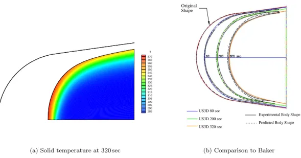
Figure 5 plots the solid grid and temperature distribution after 320 seconds of simulated exposure. Note that the grid retains its initial shape, but has been compressed to accommodate the nearly 2 inches of recession. There is no sign of surface instabilities in the grid. The temperature profile in the solid camphor varies extremely slowly, and the surface conditions reach a quasi-equilibrium state with a very slow change in the maximum temperature after about the first 20 seconds of the simulation. Thus, it is possible that larger time solid time steps could have been taken after the initial transient. Figure 5 overlays the present simulation (color lines) with the experimental data of Baker (solid black lines). (One thing to note here is that the image taken from the scanned 1972 AIAA paper does not have a 1:1 aspect ratio; it was scaled so that the “original shape” curve overlays the actual initial shape of the test article.) The comparison is very favorable, with the stagnation point recession captured, as well as the variation with time of the entire profile. T 370 365 360 355 350 345 340 335 330 325 320 315 310 305 300 295 290 285
(a) Solid temperature at 320 sec
Original Shape
Experimental Body Shape Predicted Body Shape US3D 80 sec
US3D 200 sec US3D 320 sec
(b) Comparison to Baker
Figure 5. Coupled shape-change simulation of the Baker camphor low-temperature ablator experiment.
VII.B. Detached Eddy Simulation of Capsule Wake Dynamics
The development of low-dissipation, high-order numerical methods for hypersonic flows enables new types of flow simulations. Conventional upwind methods are robust and reliable, but they have large levels of numerical dissipation, making them unsuitable for the simulation of unsteady flows. Furthermore, they are typically only second-order accurate, which introduces phase error in the solution of transient flows. In this section, the fourth-order accurate kinetic energy consistent numerical flux discussed above is used to simulate the flow over a spherical capsule geometry at Mach 6 conditions. The focus is on the unsteady behavior of the wake and the prediction of the base pressure and heat transfer rate. Additional details are available in previous publications,49, 50 as well as for capsule simulations at lower Mach number.51
shock tunnel.52 The capsule was mounted on a cylindrical sting, and 35 pressure and 39 heat flux gauges were
distributed over the back shell. The model was tested at an angle of attack of 28◦
and a range of Reynolds numbers, but only the highest Reynolds number condition is considered here. The free-stream conditions were M∞ = 6.41,ρ∞= 0.19 kg/m3, andT∞= 73.6 K, resulting in a Reynolds number of 10.8×10⁶ based
on the model diameter of 0.254 m. The turbulent boundary layers are modeled with the detached eddy simulation (DES) approach, in which the near-wall boundary layer flow is represented with a RANS model (in this case, Spalart-Allmaras) and the outer flow turbulent dissipation is modeled with a simple isotropic dissipative model.22 This hybrid RANS / large-eddy simulation (LES) approach is expected to work well
for highly turbulent flows with a clearly defined region of separated flow.
The computational grids used for the simulations were made using the GridPro software;53 these grids
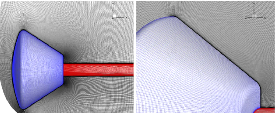
are composed of many hexahedral blocks with local refinement to resolve key regions in the wake and shear layers. The baseline grid contains about 10 million elements, and a finer grid with 56 million elements was used to assess grid convergence. Figure 6 shows two views of the baseline grid on the capsule and sting surfaces, as well as the grid in the plane of the pitch axis.
The simulations presented here were performed with three variations of the numerical flux methods discussed above: the second-order accurate modified Steger-Warming upwind fluxes and the second- and fourth-order accurate kinetic energy consistent approach. A second-order accurate implicit backward differ-ence time integration method was used with a time step corresponding to a CFL of 10. Each baseline grid simulation requires about 100 hours on 128 compute cores to obtain 100 flow times of statistics.
The high Reynolds number flow creates a highly dynamic wake with a large range of length scales. To visualize the flow field, isosurfaces of the second invariant of the velocity gradient tensor are plotted in Figure 7; the shading represents variations in the local streamwise velocity. Isosurfaces of this quantity visualize regions of vortical or swirling motion. Here, the second-order upwind, second-order KEC, and fourth-order KEC simulations on the baseline grid are shown. Note the difference in the range of length scales between the three simulations. Clearly, even though the second-order KEC method has the same formal order of accuracy as the upwind method, it produces a much more dynamic wake with a larger range of length scales. The fourth-order method has greater resolving power on the same grid, and this results in additional small-scale structure in the wake. The differences in the numerical methods are reflected in the instantaneous heat transfer rate on the back shell, as shown in Figure 8. The windside heating distributions are very similar (lower portion of the images) because the flow is attached and the near-wall turbulence model is dominant. However, on the leeside of the capsule and on the base near the sting, there are significant differences in the patterns of heating; this reflects the much more dynamic wake produced by the lower dissipation KEC methods. Again, the higher-order method produces additional small-scale dynamics that leave a heating imprint on the capsule back shell.
Figure 9 plots the time-averaged heat transfer rate obtained from the experiments and simulations on the capsule back shell along the leeside ray. Here, the small value ofxis at the capsule maximum diameter, and the large value ofxis on the capsule base. Note the low heat flux values in the separated region, and the higher values as the flow becomes intermittently attached near the capsule base. Additional analysis of the wake dynamics have been performed which shows that the low-dissipation, high-order numerical methods are significantly more consistent with the experimental measurements of unsteady heat flux in the separated wake.49
VII.C. Dynamic Simulations of Entry Capsules
The robust infrastructure within US3D for moving the computational mesh has been leveraged to perform dynamic simulations of blunt-body entry vehicles in order to characterize their dynamic stability.54
Tra-ditional blunt-body entry vehicle shapes used in spacecraft applications, such as spherical (Apollo) or 70◦
sphere-cone (Mars probes), are known to become dynamically unstable in the low-supersonic to transonic portions of their descent. Characterization of the dynamic stability is currently done exclusively through experiment, and primarily ballistic range campaigns that carry high uncertainties. The dynamics solver
Figure 6. Two views of the baseline (10 million element) computational grid on surface of capsule (blue) and sting (red), and in the capsule pitch-plane (black).
(a) Second-order upwind (b) Second-order KEC (c) Fourth-order KEC
Figure 7. Isosurfaces of the second invariant of the velocity gradient tensor computed with the baseline grid and different numerical flux functions; colored by streamwise velocity.
(a) Second-order upwind (b) Second-order KEC (c) Fourth-order KEC
Figure 9. Time-averaged heat flux to capsule back shell on the leeward ray.
module implemented within US3D, combined with the low-dissipation numerics that allow for more accu-rate simulation of unsteady flows, could enable accuaccu-rate and efficient numerical prediction of the dynamic performance of entry vehicles.
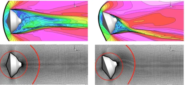
Briefly, the approach for performing a dynamic simulation is to define three zones in the mesh around the entry vehicle. The first zone, nearest the body, rotates rigidly along with the body under the influence of aerodynamics loads from the fluid dynamics solution. The second zone deforms to accommodate the rigid body motion, while the third zone which included the outer boundary remains fixed. This approach is exemplified in Figure 10 where we show the method applied to the Mars Science Laboratory (MSL) entry vehicle. The boundaries between the three aforementioned zones are highlighted here in red. The two images on the left show the nominal grid and flow solution with the capsule at 0◦
angle-of-attack, while the images on the right show the capsule pitched to 20◦
angle-of-attack. An important feature of this approach is that it maintains grid alignment with important flow features, in this case the unsteady wake of the vehicle.
Figure 10. Example of the grid motion methodology applied to the MSL ballistics range model. The left images show the capsule at0◦ angle-of-attack; The right images show the same at20◦angle-of-attack.
As the simulation is run, the body oscillates due the aerodynamic loads from the time-accurate CFD solution. Some example trajectories for the MSL ballistic range model55 at Mach 3.5 conditions are shown
in the left side of Figure 11. For each of these trajectories, the model was released from an initial angle-of-attack, as indicated in the plot, and constrained to oscillate in a single degree-of-freedom. From these trajectories, and after assuming an aerodynamic model, we can compute the relevant dynamic derivatives such asCmq(the pitch damping) as seen in the right side of Figure 11. Analysis of many different trajectories
then allows one to reconstruct the full pitch damping curve; the pitch damping curve from the ballistic range experiment is shown here by the dashed line. It should be noted that computing the dynamic derivatives is non-trivial and is highly sensitive to the choice of model and method of data reduction. For further detail the reader is referred to Sternet al.54 and its accompanying references.
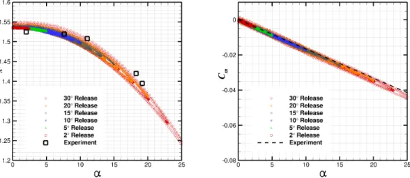
Figure 11. Example trajectories for the MSL ballistic range model along with the reconstructions based on the computed aerodynamic coefficients (left). Pitch damping coefficient as a function ofαcomputed from several different trajectories.
Figure 12. Computed and experimental axial force coefficient (left), and pitching moment coefficient (right), for the MSL capsule ballistic range model at Mach3.5.
This capability can also be used to perform angle-of-attack sweeps for building databases of static aero-dynamic coefficients. Because we are continually computing the aeroaero-dynamic loads on the vehicle for the dynamic simulation, as a byproduct we are able to output the static aerodynamic coefficients, such as lift, drag, and moment, in terms of the angle-of-attack. Examples of the axial force coefficient and the pitching moment coefficient are shown in Figure 12. The experimentally obtained coefficients are plotted here as well, and we see very good agreement between simulation and experiment.
Finally, we can also use this capability to gain insight into the mechanisms which lead to dynamic instability. One such mechanism that has been proposed56is a result of a phase lag between the forebody and
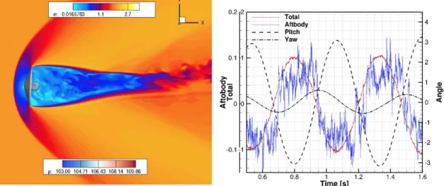
aftbody pitching moments. Because we can track surface pressures at any point along the body throughout the simulation, we are therefore able to see phenomena such as this, which would be prohibitively difficult if not impossible to track in an experiment. Figure 13 shows the computed trajectory for an idealized deployable aeroshell shape.57 Here we have plotted the pitching moment applied to aftbody alone along
with the total moment. It can be seen in this figure that the aftbody moment is lagging the total moment by some small phase angle, and we can see that there is slight amplitude growth in both the pitch and yaw angle over this time period. Having the ability to perform these types of analyses has the potential to facilitate the exploration and development of different aeroshell shapes which may improve dynamic stability.
Figure 13. Slice contours of Mach and surface pressure from a dynamic simulation of an idealized deployable aeroshell at Mach 2.0 (left). Portion of the trajectory of the pitch and yaw angle, along with the aftbody and total pitching moment (right).
VII.D. Simulation of Instability Growth on an Elliptic Cone
In this section, we use the sixth-order accurate kinetic energy consistent numerical flux discussed above to simulate the flow over a 4:1 elliptical cone at Mach 8 conditions. (Flow conditions: ρ∞ = 0.03487 kg/m3, T∞= 56.7 K, andu∞= 1208 m/s; the cone is 24 cm in length, andReL= 3.56×10⁶.)
The present simulations were motivated by the experiments of Huntley and Smits,58and build on previous
work by Bartkowiczet al.59 In that work, a spectrum of acoustic disturbances was added to the free-stream to mimic the acoustic environment of experiment. Growth of a wide variety of disturbances was observed and similar behavior of the separated symmetry plane flow was found between experiments and simulations. Here, we simplify the simulations by adding a single acoustic disturbance to the free-stream flow. This allows a more controlled analysis of how the flow field amplifies acoustic disturbances as a function of the disturbance frequency.
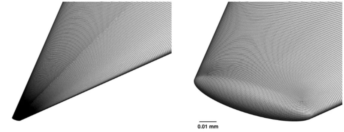
The most difficult aspect of these simulations is the development of the computational grid. The experi-mental elliptical cone geometry had a very sharp nose tip, making it difficult to resolve the flow length scales near the tip, while resolving the spatial and temporal variations associated with the acoustic disturbances. Figure 14 plots two images of the grid near the nose tip; the grid has a total of 82 million elements, with 130 elements in the wall-normal direction. Great care was take to carefully align the grid with the bow shock wave to reduce error. One critical element of the grid generation was to round the trailing edge of the body so that the flow would accelerate to supersonic speed before leaving the computational domain. This prevents any perturbations at the outflow boundary from feeding upstream and contaminating the flow.
The computations were carried out in two steps. First the flow field was converged to steady-state with an upwind flux method; the grid was aligned with the bow shock and the solution re-converged. This process was repeated until the grid was no longer changing during the grid-alignment procedure. Then acoustic perturbations were added and the flow field simulated using the sixth-order kinetic energy consistent method and second-order accurate time integration. In this phase of the simulations, the time step was taken to be 7.8 ns, corresponding to a global CFL number of 200. (This is the ratio of the computational time step to the stable time step for an explicit method.) Because of the huge variation in the length scales of the geometry, the large non-dimensional time step only applies to elements in the vicinity of the nosetip. For each case, the flow was simulated over at least 5 complete domain flow-through times.
Linear stability theory was used to estimate the most unstable frequencies for the flow on the major-axis centerline. It was found that there is strong second-mode (acoustic disturbance) growth for frequencies ranging from about 50 kHz to 400 kHz. The higher frequencies are amplified near the nosetip, and then decay. Therefore, we focused on the lower frequencies identified by this analysis. The perturbations to the free-stream were added at a level ofρ′
/ρ∞= 1.0×10
−3, and a fast acoustic wave was assumed.
Figure 14. Surface grid for elliptic cone near nosetip.
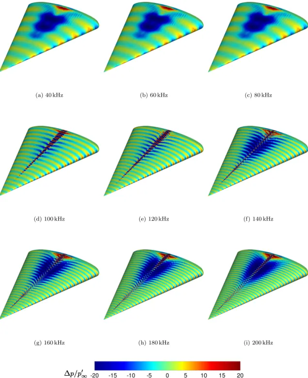
Figure 15 plots instantaneous pressure fluctuation levels for fast acoustic disturbances at a range of fre-quencies between 40 and 200 kHz. The bow shock amplifies the free-stream disturbances by different factors, depending on the local normal shock Mach number. This accounts for the larger pressure perturbation levels along the leading edge of the cone. It should be noted that the range of contour values has been reduced to help visualize the flow – the actual minimum and maximum surface pressure fluctuation levels are sig-nificantly larger than plotted here (shown below). Note that the acoustic disturbances are not appreciably amplified (nor do they decay) on most of the body surface. However, on the major-axis centerline, there is significant amplification and distortion of the plane acoustic waves. Notably, there is a region where the mean surface pressure is decreased (the large blue regions in the plots).
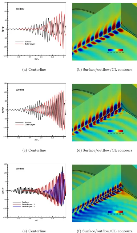
Figure 16 focuses on 3 cases: 100, 120, and 180 kHz. The line plots show centerline instantaneous pressure fluctuations, and the contour plots are on the body surface, on the major-axis centerline, and at the trailing edge of the cone. In the outflow plane, the sonic line and boundary layer edge are plotted as the black lines. At this condition, the sonic line is close to the surface, and most of the boundary layer is supersonic.
Let us first consider the 100 kHz case. In the contour plot, focus on the symmetry plane; note that in the subsonic portion of the boundary layer there are a series of alternating values of pressure. There are similar pressure variations in the supersonic region of the lifted boundary layer. In the line plot for this case, the black line is the centerline surface pressure difference – note the initial growth of the pressure fluctuations, followed by decay. The red line is the pressure difference extracted from the flow field through the approximate minima and maxima of pressure in the supersonic part of the boundary layer. Note that the near-wall pressure disturbances transfer their energy to the outer-layer disturbances, resulting in rapid disturbance growth. These two modes remain perfectly out of phase with one another until they reach the domain outflow.
At 120 kHz, there is a similar behavior, except that the boundary layer is tuned to the disturbances slightly differently. Here, the near-wall disturbance grows, and then begins to transfer energy to the outer-layer mode which grows until it flows out of the domain. However, the near wall mode has a second region of growth, presumably due to coupling and energy transfer from the higher energy outer layer disturbance. A much more complex footprint is left on the cone surface due to this modal interaction.
Finally, at 180 kHz the centerline disturbance growth is even more complicated. Here, there is rapid subsonic, near-wall growth which saturates on the first 60% of the cone. Its energy is transferred to an outer-layer mode which grows rapidly. Then a new outer-layer mode is excited (plotted in blue), which grows at the same time that the near-wall mode is also growing. Thus, there is a complicated process of inter-mode energy transfer as the boundary layer varies and becomes tuned or detuned to the disturbance frequency. It is unlikely that this process could be discovered with a conventional stability analysis because it would not identify this modal coupling.
Also note in Figure 15 that there is possible evidence of the crossflow instability at the lower excitation frequencies. This appears as striations in the surface pressure in the aft mid-span region of the cone. Plots of surface shear stress and heat flux also show variations characteristic of the crossflow instability; interestingly, it is not excited at the higher disturbance frequencies.
These simulations illustrate the power of large-scale time-accurate simulations of hypersonic flows. The high-order, low-dissipation numerical method permits new flow features to be identified to augment conven-tional means of studying hypersonic flow physics.
VIII.
Summary and Conclusions
The University of Minnesota / NASA US3D code has reached a level of maturity that it is ready to be used for the simulation of aerothermal and hypersonic flows. The code has a unique combination of grid flexibility, high-temperature physical models, advanced boundary conditions, turbulence models, numerical flux functions, and explicit and implicit time integration methods. US3D can be used for coupled flow and material response simulations, including ablation and fluid-structure interactions. US3D is designed for large-scale parallel machines and has been shown to scale well for grids of hundreds of millions of grid elements. Users can augment the capabilities of US3D to add boundary conditions, initialize the flow in a particular fashion, modify the flux function, or use a custom set of transport properties, for example. It has a powerful set of post-processing tools for plotting and analyzing large CFD datasets.
US3D has many of the same capabilities as the NASA DPLR code, but has several features that make it more powerful and general. The unstructured grid formulation allows the use of non-hexahedral elements for complicated geometries; for aerothermal applications it permits the use of hexahedral element grids with complex block topologies with a massive number of grid blocks. The low-dissipation, high-order numerical methods permit new types of unsteady hypersonic flows to be studied using detached-eddy simulations, wall-modeled large-eddy simulations, and direct numerical simulations. Novel implicit methods can dramatically
(a) 40 kHz (b) 60 kHz (c) 80 kHz
(d) 100 kHz (e) 120 kHz (f) 140 kHz
(g) 160 kHz (h) 180 kHz (i) 200 kHz
x / L p / p ’ 0 0.2 0.4 0.6 0.8 1 -150 -100 -50 0 50 100 150 Surface Outer Layer 100 kHz
(a) Centerline (b) Surface/outflow/CL contours
x / L p / p ’ 0 0.2 0.4 0.6 0.8 1 -150 -100 -50 0 50 100 150 Surface Outer Layer 120 kHz
(c) Centerline (d) Surface/outflow/CL contours
x / L p / p ’ 0 0.2 0.4 0.6 0.8 1 -150 -100 -50 0 50 100 150 Surface Outer Layer - 1 Outer Layer - 2 180 kHz
(e) Centerline (f) Surface/outflow/CL contours
Figure 16. Pressure difference on centerline surface and outer layer(s) (left); pressure difference contours (right) for 100,120, and180 kHzacoustic disturbances.
reduce the cost of simulating flows with a large number of chemical species, and for certain problems a Newton solver reduces the cost of parameter studies. Time-accurate grid deformation methods enable a wide range of multi-physics flow simulations. The examples discussed illustrate several types of advanced simulations that can be conducted with the US3D code.
Acknowledgments
We would like to thank Joseph Brock, Eric Stern, and Loretta Trevi˜no for providing simulation results for the paper. This work was sponsored by the Air Force Office of Scientific Research under grants FA9550-10-1-0563 and FA9550-12-1-0064, the Department of Defense National Security Science & Engineering Faculty Fellowship, and NASA through the Fundamental Aeronautics Program. The Department of Defense HPCMO PETTT Program supported the development of the node-based partitioning. Model development was sup-ported by the NASA Entry Systems Modeling Project within the Game Changing Development Program. Dr. Barnhardt is supported through NASA Contract NNA10DE12C with ERC Inc. The views and conclu-sions contained herein are those of the authors and should not be interpreted as necessarily representing the official policies or endorsements, either expressed or implied, of the funding agencies or the U.S. Government.
References
1Lee, J.H., “Basic Governing Equations for the Flight Regimes of Aeroassisted Orbital Transfer Vehicles,” Thermal Design of Aeroassisted Orbital Transfer Vehicles,ed. H.F. Nelson,Progress in Aeronautics and Astronautics,Vol. 96, pp. 3-53, 1985.
2
Gnoffo, P.A., R.N. Gupta, and J.L. Shinn, “Conservation Equations and Physical Models for Hypersonic Air Flows in Thermal and Chemical Nonequilibrium,” NASA TP-2867, 1989.
3
Candler, G.V. and R.W. MacCormack, “The Computation of Hypersonic Ionized Flows in Chemical and Thermal Nonequilibrium,”Journal of Thermophysics and Heat Transfer,Vol. 5, No. 3, pp. 266-273, 1991.
4
Nompelis, I., T. Drayna, and G.V. Candler, “Development of a Hybrid Unstructured Implicit Solver for the Simulation of Reacting Flows Over Complex Geometries,”AIAA 2004-2227,June 2004.
5
Nompelis, I., T. Drayna and G.V. Candler, “A Parallel Unstructured Implicit Solver for Hypersonic Reacting Flow Simulation,”AIAA 2005-4867,June 2005.
6
Wright, M.J., D. Bose, and G.V. Candler, “A Data-Parallel Line Relaxation Method for the Navier-Stokes Equations,”
AIAA Journal,Vol. 36, No. 9, 1998, pp. 1603-1609. 7
Gordon, S., and B.J. McBride, “Computer Program for Calculation of Complex Chemical Equilibrium Compositions and Applications, I. Analysis,” NASA RP-1311, Oct. 1994.
8
McBride, B.J., and S. Gordon, “Computer Program for Calculation of Complex Chemical Equilibrium Compositions and Applications, II. Users Manual and Program Desciption,” NASA RP-1311-2, June 1996.
9
Millikan, R.C. and D.R. White, “Systematics of Vibrational Relaxation,”J. Chem. Phys.,Vol. 39, pp. 3209-3213, 1963. 10
Park, C., “Review of Chemical-Kinetic Problems of Future NASA Missions I - Earth Entries,”Journal of Thermophysics and Heat Transfer,Vol. 7, No. 3, pp. 385-398, July 1993.
11
Gupta, R.N., J.M. Yos, R.A. Thompson, and K.-P. Lee, “A Review of Reaction Rates and Thermodynamic and Transport Properties for an 11-Species Air Model for Chemical and Thermal Nonequilbrium Calculations to 30000 K,” NASA RP-1232, Aug. 1990.
12
Wilke, C.R., “A Viscosity Equation for Gas Mixtures,”J. Chem. Phys.,Vol. 18, pp. 517-519, 1950. 13
Armaly, B.F., and Sutton, L., “Viscosity of Multicomponent Partially Ionized Gas Mixtures,” AIAA Paper 80-1495, July 1980.
14
Ramshaw, J.D., and C.H. Chang, “Ambipolar Diffusion in Two-Temperature Multicomponent Plasmas,”Plasma Chem-istry and Plasma Processing,Vol. 13, No. 3, 489-498, 1993.
15
Ramshaw, J.D., and C.H. Chang, “Ambipolar Diffusion in Two-Temperature Multicomponent Plasmas,”Physical Re-view E,Vol. 53, No. 6, 6382-6388, 1996.
16
Candler, G.V., “Hypersonic Nozzle Analysis Using an Excluded Volume Equation of State,”AIAA 2005-5202, June 2005.
17
Spalart, P.R., and Allmaras, S.R., “A One-Equation Turbulence Model for Aerodynamic Flows,” AIAA-1992-0439, Jan. 1992.
18
Catris, S., and B. Aupoix, “Density Corrections for Turbulence Models,” Aerospace Science and Technology,Vol. 4, 2000, pp. 1-11.
19