Optimal Operational Monetary Policy Rules in an Endogenous Growth Model: a calibrated analysis

Full text

(1)KIER DISCUSSION PAPER SERIES KYOTO INSTITUTE OF ECONOMIC RESEARCH Discussion Paper No. 663 “Optimal Operational Monetary Policy Rules in an Endogenous Growth Model: a calibrated analysis”. Hiroki Arato. January 2009. KYOTO UNIVERSITY KYOTO, JAPAN.

(2) Discussion Paper No.663 Optimal Operational Monetary Policy Rules in an Endogenous Growth Model: a calibrated analysis. Hiroki Arato. January 5, 2009. Kyoto Institute of Economic Research Kyoto University.

(3) Optimal Operational Monetary Policy Rules in an Endogenous Growth Model: a calibrated analysis∗ Hiroki Arato† January 5, 2009. abstract This paper constructs an endogenous growth New Keynesian model and considers growth and welfare effect of Taylor-type (operational) monetary policy rules. The Ramsey equilibrium and optimal operational monetary policy rule is also computed. In the calibrated model, the Ramseyoptimal volatility of inflation rate is smaller than that in standard exogenous growth New Keynesian model with physical capital accumulation. Optimal operational monetary policy rule makes nominal interest rate respond strongly to inflation and mutely to real activity, as in standard New Keynesian model. Growth-maximizing operational monetary policy is not identical to optimal operational monetary policy. Welfare cost of responding to real activity is two or three times larger than that of exogenous growth New Keynesian model.. Keywords: Monetary policy, Sticky price, Endogenous growth JEL classification: E31, E52, O41. ∗ I appreciate many helpful comments and suggestions received from my adviser Tomoyuki Nakajima. I am also grateful to Takayasu Matsuoka and workshop participants at Osaka University. Any remaining errors are the sole responsibility of my own. This study is financially supported by the research fellowships of the Japan Society for the Promotion of Science for young scientists. † Japan Society for the Promotion of Science and Graduate School of Economics, Kyoto University. E-mail address: hirokiarato@gmail.com.

(4) 1. Introduction. In this paper we construct an endogenous growth model with Calvo (1983)type nominal rigidities and consider growth and welfare effect of Taylor-type (operational) monetary policy rules. There are some reasons why it is important to endogenize growth rate of output in New Keynesian model. One reason is from the positive point of view. It is known that some stochastic endogenous growth model offer improvements over simple (exogenous growth) Real Business Cycle models. For example, Jones et al. (2005a) show that simple one-sector endogenous growth model in which engines of growth are physical and human capital can explain some of U.S. business cycle properties better than a standard Real Business Cycle model, specifically about volatility of labor supply and about persistence of growth rate. Comin and Gertler (2006) also show that R&D endogenous growth model with uncertainty accounts for the medium term properties of business cycles well. Hence, the endogenous growth models with nominal rigidities have the potential abilities accounting the business cycle properties better than the existing New Keynesian models. As a first step, we use the convex model of endogenous growth developed by Jones et al. (2005a). The other reason is from normative point of view. Lucas (1987) shows that the cost of business cycles is much less than that of growth. It is well known that his claim is strongly robust,1 but it does not imply that fluctuations are negligible for the macroeconomics at all, because even if fluctuations itself has the small welfare effect, fluctuations can affect the long-run growth. In stochastic endogenous growth literature, Jones et al. (2005b) show that convex models of endogenous growth has the effect of uncertainty on long-run growth. Moreover, when capital accumulation technology is concave, fluctuation of investment lowers mean growth rate, as showed in Barlevy (2004b). Although their analysis does not consider nominal rigidities, by incorporating nominal rigidities into their model monetary policy has growth effect. That is, different monetary policy rules alter not only mean level of output but mean growth rate of output even when deterministic steady state is identical. Hence there is some possibilities to change the inflation-output tradeoff. For example, Blackburn and Pelloni (2005) analytically show that optimal money-supply feedback rule is identical to the growth-maximizing money supply rule in a learning-by-doing endogenous growth model with nominal rigidities of wage contracts in one-period-advance. For these reasons, endogenizing productivity growth can be thought to be important for the analysis of business cycle and monetary stabilization policy. Most of studies about short-run monetary policy (New Keynesian approach), however, have been ignored the effect of monetary policy on long-run economic growth.2 We conjecture that the reason is purely technical issue. In most of New Keynesian studies, they approximate to the policy functions around nonstochastic steady-state up to first-order. In those linear models, unconditional mean of endogenous variables are idendical to the non-stochastic steady-state value. Hence, in addition that long-run growth rate is endogenous, higher-order 1 Excellent. surveys in the literature are Lucas (2003) and Barlevy (2004a). analysis studying the relationship between money and growth under uncertainty, see Gomme (1993), Dotsey and Sarte (2000), Blackburn and Pelloni (2004), and Varvarigos (2008). In contrast to them, we consider the growth and welfare effect in cashless economy with Calvo-type nominal rigidities. 2 For. 1.

(5) approximation is needed for the model to show the growth effect of monetary policy. To fix the problem, we use the computation method which approximating to the policy function up to second-order developed by Schmitt-Grohe and Uribe (2004). Their method enables us to address the relationship between monetary stabilization policy and long-run growth. In this paper, we consider that whether optimal tradeoff between inflation and output would be altered by an introduction of endogenous growth. In order to see that, first we compute optimal inflation volatility at the Ramsey equilibrium in a endogenous growth New Keynesian model and compare its volatility to the one in the exogenous growth counterpart, that is, a standard New Keynesian model with physical capital accumulation. This analysis shows that optimal inflation volatility is smaller in the endogenous growth model than in the exogenous growth counterpart. This result suggests that in the endogenous growth model monetary authority should stabilize inflation more strongly than in the exogenous growth model. Second, we compute optimal operational monetary policy rule, which is defined as the walfare-maximize nominal-interest-rate feedback rule. We show that in the endogenous growth model optimal operational monetary policy rule makes nominal interest rate respond strongly to inflation and mutely to real activity, that is, output growth or cyclical component of output. We also show that the optimal operational monetary policy rule is not identical to the growth-maximizing interest-rate feedback rule. Thus, their conclusion in Blackburn and Pelloni (2005) is not robust to New Keynesian sticky price assumption. Finally, we compute welfare cost of monetary policy which responds to real activity and show that its welfare cost measured in income unit is two or three times larger than in the exogenous growth model. These results suggest that in the endogeneous growth model, on the one hand, sticky price distortion has large welfare effect through growth effect, on the other hand, negative growth and welfare effect which is caused by output fluctuation and investment adjustment costs is relatively small. The most related researches to this paper is Schmitt-Grohe and Uribe (2005), Schmitt-Grohe and Uribe (2007), Faia (2008), and Kollman (2008). These studies compute the Ramsey optimal and/or optimal operational monetary policy rules under medium-scale (but exogenous growth) New Keynesian models by using second-order approximation. Schmitt-Grohe and Uribe (2007) and Kollman (2008) consider fiscal policy as well as monetary policy. Their common conclusion is that optimal monetary policy is virtually inflation stabilization policy. Our main contribution is to show that their finding is robust to an extension to endogenous growth and that growth-maximizing policy does not necessarily maximize welfare, unlike Blackburn and Pelloni (2005). This paper is organized as follows. In the next section, we present an stochastic endogenous growth model with nominal rigidities and calibrate the model. Section 3 analyzes the Ramsey equilibrium and compare the outcome to that of the exogenous growth model. Section 4 considers the growth and welfare effect of some operational monetary policy rules and compute optimal operational monetary policy rules. Section 5 concludes this paper.. 2.

(6) 2. The Model. The model is based on a stochastic one-sector endogenous growth model in which engines of growth are physical and human capital accumulation and in which labor supply is endogenized as human capital utilization, as in Jones et al. (2005a). We extend their model by incorporating monopolistic competition in product markets, nominal rigidities in the form of sluggish price adjustment, and real rigidities in the form of investment adjustment costs of human and physical capital.. 2.1. Final-Good Producers. At time t, a perfectly competitive, representative firm produces a final good, Yt , combining a continuum of differentiated intermediate goods, indexed by i ∈ (0, 1). The firm can use the technology represented by CES aggregator, [∫. 1. Yt =. (Yit ). θ−1 θ. θ ] θ−1. di. ,. (1). 0. where θ > 1, and Yit denotes the input of intermediate good i at time t. Given its nominal output price, Pt , and its nominal input prices, Pit , the firm maximizes its profit. The demand for intermediate good i is derived by profit maximization as ( )−θ Pit Yit = Yt . (2) Pt Hence θ denotes price elasticity of demand for good i. Substituting (2) for (1), we can describe the nominal price index Pt by the nominal input prices Pit : [∫. 1 ] 1−θ. 1. Pt =. (Pit ). 1−θ. di. .. (3). 0. 2.2 2.2.1. Intermediate-Goods Firms Technology. Intermediate good i is produced by a monopolistic firm i. The firm can access the technology described by Cobb-Douglas production function, Yit = At (Kit )α (Zit )1−α ,. (4). where 0 < α < 1, which denotes aggregate share of physical capital. Here, Kit and Zit denote physical capital services and effective labor used to produce the intermediate good i at the time t, and At denotes aggregate productivity, which follows an exogenous stochastic process described later. 2.2.2. Factor Prices and Real Marginal Cost. Given the real wage rate wt and real rate of return on physical capital rtK , firm i minimizes its production cost, rt Kit + wt Zit , subject to (4). The first-order. 3.

(7) conditions are given by )α−1 Kit = αAt mcit , Zit ( )α Kit wt = (1 − α)At mcit , Zit (. rtK. (5) (6). where mcit denotes the Lagrange multiplier for (4), hence it represents the real marginal cost of production which firm i faces. From these equations, we obtain wt 1 − α Kit = , α Zit rtK. (7). that is, the ratio of physical capital to effective labor demand are identical across firms. Hence the real marginal cost is also in common among firms, so that the subscript representing the firm index i can be dropped. 2.2.3. Calvo Pricing. We assume price stickiness following Calvo (1983) and Yun (1996), that is, each period a fraction ξp ∈ [0, 1) of randomly chosen firms cannot reoptimize the nominal price of their producted good. The nominal price of good i is set according to the following rule: { P̃t if the firm can set their price optimally, Pit = (8) Pi,t−1 otherwise. Hence, profit maximization problem are formulated as (  )1−θ ( )−θ ∞ ∑ P̃ P̃ t t max Et dt,t+s Pt+s ξps  Yt+s − Yt+s mct+s  . P P t+s t+s s=0 The first-order condition with respect to P̃t is   ( )−θ ( )−θ−1 ∞ ∑ P̃ P̃ θ − 1 t t Et − mct+s  = 0. dt,t+s ξps Yt+s  θ P P t+s t+s s=0. (9). (10). Define Xt1 and Xt2 as Xt1. ≡ Et. ∞ ∑. ( dt,t+s ξps Yt+s. s=0. Xt2. ≡ Et. ∞ ∑. ( dt,t+s ξps Yt+s. s=0. P̃t Pt+s P̃t Pt+s. )−θ−1 mct+s ,. (11). )−θ ,. (12). respectively, and we obtain the recursive formulation of optimal price setting. 4.

(8) behavior, )−θ−1 p̃t 1 + ξp Et dt,t+1 Xt+1 , = πt+1 p̃t+1 ( )−θ p̃t 2 Xt2 = p̃−θ Y + ξ E d Xt+1 , t p t t,t+1 t πt+1 p̃t+1 θ−1 2 Xt , Xt1 = θ Xt1. (. p̃t−θ−1 Yt mct. (13) (14) (15). where we define p̃t ≡ P̃t /Pt .. 2.3. Households. A representative household has preference which are described by the following utility function, ∞ ∑ E0 β t U (Ct , 1 − nt ), (16) t=0. with U (Ct , 1 − nt ) ≡ log Ct + ψ log(1 − nt ). (17). where Ct denotes final good consumption per capita, nt represents total hour worked per capita, β is the subjective discount rate, and where ψ is the curvature parameter of period utility. No population growth is assumed. Households own human capital Ht , and physical capital Kt . Capital accumulation equations are assumed as follows. ( Kt+1 = (1 − δK )Kt + ( Ht+1 = (1 − δH )Ht +. ItK Kt ItH Ht. )φK Kt. (18). Ht. (19). )φH. where δK and δH denote the depreciation rates of physical and human capital, and φK and φH represent the investment adjustment cost parameters for physical and human capital,3 respectively. We assume that households can access to a complete set of nominal statecontingent claims and that the effective labor is defined as product of hour worked and human capital, so that households’ intertemporal budget constraint is Et dt,t+1. Xt+1 Xt + Ct + ItK + ItH + Tt = + wt nt Ht + rtK Kt + Φt , Pt Pt. (20). where dt,s is nominal stochastic discount factor, Xt is nominal payment of statecontingent claims in period t, rtK denotes real rental rate on physical capital, Φt is real profits received from firms, and Tt denotes the lump-sum tax levied by the government. 3 We. applies identical formulation to human and physical capital accumulation because we cannot find the emperical evidence about the form of human capital invenstment technology. The study about it remains for future research.. 5.

(9) Choosing processes for Ct , nt , Xt+1 , ItK , ItH , Kt+1 , Ht+1 , households maximize (16) subject to (18), (19), (20), and the no-Ponzi game condition. Let us define the Lagrange multipliers associated with (18), (19), (20) as β t Λt qtK , β t Λt qtH , and β t Λt respectively, and we obtain the first-order conditions with respect to Ct , nt , Xt+1 , ItK , ItH , Kt+1 , Ht+1 as follows. Ct : Λt = Ct−1 ,. (21) −1. nt : Λt wt Ht = ψ(1 − nt ) , βΛt+1 Xt+1 : dt,t+1 = , Λt πt+1 ( K )φK −1 It K K , It : 1 = qt φK Kt ( H )φH −1 It ItH : 1 = qtH φH , Ht { Kt+1 :. Λt qtK. K rt+1. = βEt Λt+1. (22) (23) (24) (25) [ +. K qt+1. ( (1 − φK ). { Ht+1 : Λt qtH = βEt Λt+1. K It+1 Kt+1. [. H wt+1 nt+1 + qt+1 (1 − φH ). (. ]}. )φK + 1 − δK. H It+1. Ht+1. , (26) ]}. )φH + 1 − δH. . (27). From (23) and the definition of nominal interest rate, 1/Rt = Et dt,t+1 , we obtain the well-known Fisher relationship, 1 Λt+1 = βEt . Rt Λt πt+1. 2.4 2.4.1. (28). Government Fiscal policy. As our study focuses only on monetary policy, we assume that fiscal authority finances whole government expenditure, Gt by lump-sum tax Tt . As we assume cashless economy, the intertemporal budget constraint of the government is: Gt = Tt . Along a balanced-growth path, the share of government expenditure in aggregate demand assumed to be constant. To this end it is imposed: Gt = gt Ht , hence gt represents the government-expenditure-human-capital ratio at time t. We assume that gt follows an exogenous stochastic process described below. 2.4.2. Monetary policy. Following some rules described below, monetary authority sets the process for the nominal interest rate, Rt . 6.

(10) 2.5 2.5.1. Closing The Model Price index. By equations (3) and (8), we obtain + ξp πt θ−1 . 1 = (1 − ξp )p̃1−θ t 2.5.2. (29). Price setting. Substituting (23) into (13) and (14), ( )−θ−1 p̃t Λt+1 θ 1 = π Xt+1 , + βξp Et Λt t+1 p̃t+1 ( )−θ Λt+1 θ−1 p̃t 2 Xt2 = p̃−θ Y + βξ E π Xt+1 . t p t t Λt t+1 p̃t+1 Xt1. 2.5.3. p̃t−θ−1 Yt mct. (30) (31). Final-good market. Final-good output is used for consumption, investment of physical and human capital, and Government expenditure. Hence, final-good market clearing condition is (32) Yt = Ct + ItK + ItH + Gt . 2.5.4. Intermediate-goods markets. Market clearing condition in good market i is written as ( )−θ Pit α 1−α At Kit Zit = Yt . Pt Resource constraint with respect to physical capital is ∫ 1 Kit di = Kt .. (33). (34). 0. Resource constraint with respect to effective labor is ∫ 1 Zit di = nt Ht .. (35). 0. By (34), (35), and by the fact that, in equilibrium, capital to effective labor ratios are identical across the firms because the firm’s production function is homogeneous of degree one, we can integrate the equation (33) over all good markets. As the result we obtain aggregate resouce constraint At Ktα (nt Ht )1−α = Yt st , where we define. ∫. 1. st ≡ 0. (. Pit Pt. (36). )−θ di,. (37). or as recursive representation, θ st = (1 − ξp )p̃−θ t + ξp πt st−1 .. 7. (38).

(11) st (≥ 1) denotes the inefficiency by the price dispersion. By equations (5), (6), and by the fact that, the equilibrium capital to effective labor ratios are identical across firms, we obtain rtK = αAt Ktα−1 (nt )1−α Ht1−α mct , wt = (1 − 2.5.5. α)At Ktα (nt )−α Ht−α mct .. (39) (40). Exogenous process. The law of the motion of aggregate productivity At is assumed to be given by the following exogenous stochastic process ( ) ( ) At At−1 (41) log = ρA log + σ²A ²A t , A A 0 ≤ ρ < 1, ²A t ∼ N (0, 1), where A is the value of productivity at deterministic steady state and where σ²A is standard deviation of the stochastic disturbance. Government-expenditure-human-capital ratio gt is assumed to be given by the following stochastic process ( ) ( ) gt gt−1 log = ρg log + σ²g ²gt , (42) g g 0 ≤ ρ < 1, ²gt ∼ N (0, 1), where g is the value of government-spending-human-capital ratio and where σ²g is standard deviation of the stochastic disturbance.. 2.6. Competitive Equilibrium. We define a competitive equilibrium as a set of processes Ht , Ct , Λt , nt , πt , Yt , ItK , ItH , Xt1 , Xt2 , mct , p̃t , Kt , st , rtK , wt , qtK , and qtH satisfying (15), (18), (19), (21), (22), (24)-(32), (36), and (38)-(40), given the nominal interest rate policy process Rt , exogenous aggregate productivity stochastic process At , exogenous government spending stochastic process gt , and initial conditions H0 , K0 , A0 , g0 , s−1 .. 2.7. Calibration. The parameter values are summarized in Table 1. The model is calibrated by the following way. The time unit is assumed to be one quarter. We set δK to be 0.025, δH to be 0.005, α to be 0.36, θ to be 6, ξp to be 0.75, and g to be 0.17. These values are in the ranges of parameter values used existing studies. β, ψ and A are estimated by using deterministic steady-state conditions4 and the following restrictions. We impose gross inflation rate at deterministic steady-state, π, to be 1.0421/4 , steady-state output growth rate is 0.45 percent per quarter, steady-state hour worked, n, to be one half,5 and quarterly real interest rate to be one percent. 4 The. deterministic steady state means an balanced-growth equilibrium given σ²A = σ²g = 0. log utility, n = 0.5 implies unit Frisch elasticity of labor supply.. 5 Given. 8.

(12) Investment adjustment cost parameters, φK , φH are estimated so that standard deviation of growth rate of physical capital investment is three times larger than that of growth rate of output, and that standard deviation of growth rate of broad consumption6 is as half as that of growth rate of output. Following the estimate by Schmitt-Grohe and Uribe (2006), the parameters governing stochastic process of government spending, ρg and σ²g are set to be 0.87 and 0.016 respectively. Following Schmitt-Grohe and Uribe (2006), the parameters governing stochastic process of productivity, ρA and σ²A are calibrated as follows. We assume that monetary policy take the form of a simple Taylor-type rule whereby the current nominal interest rate is set as a function of contemporaneous inflation and output. We then pick the four parameters describing the technology shocks and the monetary policy rule so that the model matches the standard deviation and serial correlation of output growth and inflation observed in the U.S. economy. For comparative purpose, we also consider the exogenous growth counterpart of our model. In the exogenous growth model, the growth rate of human capital, γtH , is exogenously 1.0045 and human capital investment is zero in all t. In this economy, φH and δH no longer affect the equilibrium. Steady-state productivity parameter, A, is arbitrary in the exogenous model. Thus, without loss of generality, we set A to be 1. Following Schmitt-Grohe and Uribe (2007), we set ρA to be 0.8556 and σ²A to be 0.0064. Given those restrictions, We calibrate the exogenous growth model by the same strategy as in the endogenous growth model.. 3. Ramsey Policy. As a benchmark, we consider Ramsey monetary policy before growth and welfare effect of interest rate feedback rules, which is a main objective in this paper. Ramsey planner maximizes households’ utility subject to competitive equilibrium conditions. In choosing ramsey policy, the planner is assumed to honor commitments made in the past, according to ’optimal from timeless perspective’ in Woodford (2003).. 3.1. Ramsey Steady State: Optimal Long-run Rate of Inflation and Growth. We refer to the balanced-growth path of a Ramsey equilibrium without uncertainty as the Ramsey steady state. We focus on the rate of inflation and the growth rate of output. These values at the Ramsey steady state are reported in the parentheses of Table 2. First, we find the rate of inflation at the Ramsey steady state is nil as long as the degree of price stickiness ξp is positive. The reason is straightforward. Our economy is assumed the existence of only single nominal distortion, that is, sluggish adjustment of product prices. Therefore, the optimal long-run monetary policy is that inflation rate is set to zero so that the inefficiency from relative price dispersion is eliminated. Next, under the parameters showed in table 1, changing the annual rate of inflation from 4.2 6 Following Jones et al. (2005a), we refer the sum of consumption and human capital investment as ‘broad consumption’.. 9.

(13) percent to zero rises the growth rate of output by 0.02 percentage point per year.. 3.2. Short-run Inflation-Output Tradeoff: Optimal Volatility of Inflation. In this subsection, we characterize the business cycle dynamics that arise in the stochastic steady state of the Ramsey equilibrium in order to see optimal volatility of inflation. We approximate the Ramsey equilibrium dynamics by solving a second-order approximation to the Ramsey equilibrium conditions around the Ramsey steady state, using the computation method developed by Schmitt-Grohe and Uribe (2004). In New Keynesian models, strict inflation stabilization policy, πt = 1 in all t, is not optimal because there exists tradeoff between inflation stabilization and output stabilization, that is, inflation can weaken the distortion of monopolistic competition in the short run. Schmitt-Grohe and Uribe (2005) and Kollman (2008) analyze exogenous growth New Keynesian models with capital accumalation and show that optimal volatility of inflation is very small and that strict inflation stabilization attains almost the same welfare level as the Ramsey equilibrium. Those results imply that in exogenous New Keynesian models, short-run inflation-output tradeoff is virtually resolved by inflation stabilization policy. We consider whether or not those results hold in our endogenous growth model. When growth rate is endogenous, different monetary policy rules alter not only mean level of output but mean growth rate of output even when deterministic steady state is identical. This growth effect of monetary policy may alter inflation-output tradeoff and optimal volatility of inflation. Table 2 reports the means and standard deviations of inflation and output growth in the Ramsey equilibrium. On the one hand, the standard deviation of inflation in the Ramsey equilibrium is 0.027 percent in the endogenous growth model and 0.15 percent in the exogenous growth counterpart. In the endogenous growth model, the optimal volatility of inflation is only about one fifth of in the exogenous growth model. On the other hand, The standard deviation of growth rate of output in the Ramsey equilibrium is 4 percent in the endogenous growth model and 3.29 percent in the exogenous growth model. The optimal volatility of growth rate of output in the endogeous growth model is 1.2 times larger than in the exogenous growth model. Those results imply that in the endogenous growth model, inflation-output tradeoff is resolved by stronger anti-inflation stance than in the exogenous growth model. In the Ramsey equilibrium, mean inflation is virtually the same as the Ramsey steady state value. Therefore, we see that Ramsey planner keeps inflation rate virtually zero also in stochastic environment. Mean growth rate of output is also virtually the same as the Ramsey steady state. This result implies that in the Ramsey equilibrium there is very small growth effect by business cycle fluctuation. Note that it does not necessarily means growth effect is small in any competitive equilibrium. The growth effect of different monetary policy rules is investigated in the next section.. 10.

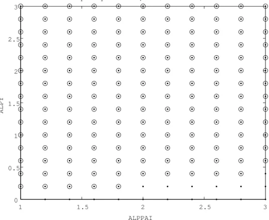
(14) 4. Growth and Welfare Effect of Operational Monetary Policy Rules. As pointed out in Schmitt-Grohe and Uribe (2005), Ramsey outcomes are mute on the issue of what policy regimes can implement them. In addition, as described in the end of previous section, our main objective is to uncover the growth and welfare effect of monetary policy but the Ramsey equilibrium give us few information about these effects. In this section, we consider growth and welfare effects of different monetary stabilization policy rules. Similar to Schmitt-Grohe and Uribe (2007), we address the ‘operational monetary policy rules’ defined as follows. An operational monetary policy rule (απ , αγ , αY ) must satisfy the following four conditions. First, nominal interest rate is set depending linearly on the rate of inflation, the level of output, and the growth rate of output. Formally, the interest-rate rule is given by: ( ) ( ) ( Y ) (π ) Rt yt γt t log = α log + α log + α log , (43) π Y γ R∗ π∗ y∗ γY ∗ where γtY and yt (≡ Yt /Ht ) is gross growth rate of output and output level, and where asterisk represents its value at the Ramsey steady state. Hence, απ , αY , and αγ govern the response of nominal interest rate to deviation of inflation, output level, and output growth from Ramsey steady state, respectively. Second, the policy coefficients απ , αγ , and αY must be in the range of [0, 3],7 though most of our results are robust to changing the size of interval. Third, an operational monetary policy rule must guarantee local uniqueness of rationalexpectation equilibrium. Fourth, the path of nominal interest rate associated with an operational monetary policy rule must not violate the zero bound of nominal interest rate. As in Schmitt-Grohe and Uribe (2005) and in SchmittGrohe and Uribe (2007), we approximate this constraint by requiring that in the competitive equilibrium two standard deviations of the nominal interest rate be less than the steady-state level of the nominal interest rate. More formally, in the competitive equilibrium characterized by an operational monetary policy, it must be satisfied that 2σR < log R∗ where σR is the standard deviation of the nominal interest rate measured in percentage point. Below we consider two alternative operational monetary policy rules. Specifically, monetary policy responding to output level, αγ = 0, and monetary policy responding to output growth, αY = 0.. 4.1 4.1.1. Growth and Welfare Effect, and Optimal Operational Monetary Policy Rule Growth Effect. Here we investigate the growth effect of monetary stabilization policy rules. Figure 1 and 2 shows the growth effect of monetary policy responding to output growth and to output level, respectively. On the one hand, when nominal interest rate respond to neither output growth nor its level, an increases of the degree 7 In. Schmitt-Grohe and Uribe (2007), they say “The size of this interval is arbitrary, but we feel that policy coefficients larger than 3 or negative would be difficult to communicate to policymakers or the public.”. 11.

(15) of response to inflation rate, απ , has little growth effect. On the other hand, we see that the growth effect varies depending on whether nominal interest rate responds to output growth or level. When nominal interest rate responds to output growth (Figure 1), growth effect is decreasing in αγ . When nominal interest rate responds to output level (Figure 2), however, growth effect is more complicated. Specifically, when αY is near but larger than 1 the growth rate of output lowers as αY increases. When αY is larger the growth rate of output rises as αY increases, though when αY is large enough for its increases to rise the growth rate of output, these policy rules are not operational because the equilibrium associated with these policy rules violate the zero bound of nominal interest rate. (See figure 3 and 4.) In both rules, the policy responding to real activity lowers the growth rate of output by at most 0.1 percentage point per year. 4.1.2. Welfare Effect and Optimal Operational Policy. Next we consider the welfare effect of monetary stabilization policy. Figure 5 and 6 shows the growth effect of monetary policy responding to output growth and to output level, respectively. Welfare cost of an operational monetary policy rule is defined as the fraction of income process in the Ramsey equilibrium that a household would be willing to give up to be as well off under the operational policy as under the Ramsey policy.8 We see from figure 5 and 6 that the policy responding mutely to real activity attains high welfare level (low welfare cost) and that its welfare level is virtually the same as in the Ramsey equilibrium. Strictly speaking, optimal operational monetary policy is απ = 3 and αγ = αY = 0. This result implies that optimal operational policy implication in existing exogenous growth New Keynesian models, in which nominal interest rate should responds strongly to inflation and mutely to real activity, is robust to our extension to endogenous growth. By comparing the growth effect (figure 1 and 2) to the welfare effect (figure 5 and 6), we find that high growth rate does not necessarily guarantee high economic welfare. If monetary authority would conduct growth maximization policy, nominal interest rate responds weakly to inflation rate. However, this policy does not only maximize welfare but is not operational because the volatility of nominal interest rate become too large in this policy (See figure. 3 and 4.). This results is one of our main findings. Blackburn and Pelloni (2005) analytically shows that optimal monetary policy is identical to growth maximization policy in a learning-by-doing endogenous growth model with wage contracts in one-period advance as nominal rigidities. However, our result shows that their conclusion is not robust. In a New Keynesian model with endogenous growth, optimal operational policy is inflation stabilization policy, which is claimed by New Keynesian literature, rather than growth maximizing policy, which is claimed by Blackburn and Pelloni (2005). 8 In Schmitt-Grohe and Uribe (2005), welfare cost is measured in consumption unit. The reason that we measure welfare cost in income unit is that in the next subsection we compare the welfare cost in our model to the one in the exogenous growth counterpart, between each of which the consumption share of aggregate demand is different. We compute welfare cost in consumption unit by the same method as in Schmitt-Grohe and Uribe (2005) and convert it into income unit by multiplication of the consumption-output ratio at the Ramsey steady state. Note that high welfare cost implies low level of welfare.. 12.

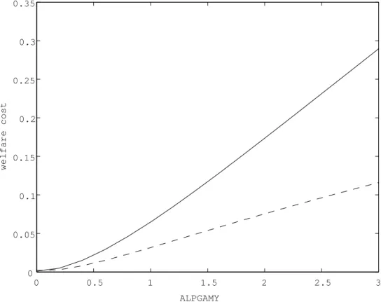
(16) 4.1.3. Welfare cost of monetary policy responding to output. In the previous subsection, we see that optimal operational monetary policy responds strongly to inflation and mutely to real activity in both of an exogenous and endogenous growth model. We then consider the difference of these two New Keynesian models. In section 3, the Ramsey optimal volatility of inflation is smaller in our endogenous growth model than in the exogenous growth counterpart. From this result, we can expect that welfare cost of the operational monetary policy rule responding to real activity result to larger welfare loss in the endogenous growth model than in the exogenous growth model. Figure 7 and 8 compare the welfare cost of responding output growth or level in the endogenous growth model to those of the exogenous growth model. By the policy responding to growth rate of output, welfare cost is about two times larger in the endogenous growth model than in the exogenous growth model. By the policy responding to level of output, welfare cost is about three times larger in the endogenous growth model than in the exogenous growth model. From results in the section 3 and this subsection, we conclude that in our endogenous growth model, inflation stabilization is more important than in the exogenous growth model from the normative point of view.. 5. Conclusion and Future Research Directions. We compute ramsey and operational optimal monetary policy in an endogenous growth model with nominal rigidities and measure the welfare cost of deviation from optimal monetary policy. As the result, in our calibrated endogenous growth model, inflation stabilization as the goal of monetary policy is more important than in standard exogenous growth New Keynesian models. Unfortunately, the complexity of the model make it difficult to uncover the exact mechanism. However, we conjecture the intuition as follows. Our endogenous growth extension adds growth effect of monetary policy from at least three directions. First, precautionary saving motive increases saving and growth rate as business cycle fluctuation is larger. Second, under sticky price assumption, inflation fluctuation reduces final good output by relative price dispersion hence investment and growth decrease. Third, fluctuation of investment decrease mean output growth through convex investment adjustment costs, showed in Barlevy (2004b). Jones et al. (2005b) show that the perfect competition version of our model has a small growth effect. Thus the first growth effect of our model would be also small. Second, in our calibration, the degree of convexity of investment adjustment costs are much smaller than those estimated by Barlevy (2004b). Therefore the third growth effect would be also small.9 After all, growth effect in our model would result mainly from sticky price distortion and its distortion is heavier by the growth effect than the exogenous growth models. There is some directions of future research. First, in this paper an endogenous growth model in which engines of growth are physical and human capital is studied. It is known that the relationship between growth and fluctuation could alter depending on engine of growth. Hence, further research is needed in order to clear that whether our conclusion is robust to different endogenous growth models, for example, R&D stochastic endogenous growth model developed by 9 In. fact, no convex investment adjustment cost does not affect our main results.. 13.

(17) Comin and Gertler (2006). Second, incorporating capital market imperfection into a stochastic endogenous growth model would give rise to strong distortion in capital accumulation and hence growth effect. Faia and Monacelli (2007) do welfare-based analysis of optimal monetary policy in an exogenous growth New Keynsian model with credit market imperfection developed by Carlstrom and Fuerst (1997). It is noteworthy to extend their model to endogenous growth model and to analysis growth and welfare effect of monetary policy.. Reference Barlevy, Gadi (2004a) “The Cost of Business Cycles and The Benefit of Stabilization: A Survey.” NBER Working Paper, No. 10926. Barlevy, Gadi (2004b) “The Cost of Business Cycles Under Endogenous Growth,” American Economic Review 94(4) , pp. 964–990. Blackburn, Keith and Alessandra Pelloni (2004) “On the Relationship between Growth and Volatility,” Economic Letters 83, pp. 123–127. Blackburn, Keith and Alessandra Pelloni (2005) “Growth, Cycles, and Stabilization Policy,” Oxford Economic Papers 57, pp. 262–282. Calvo, Guillermo (1983) “Staggered Prices in a Utility-Maximizing Framework,” Journal of Monetary Economics 12(3) , pp. 383–398. Carlstrom, Charles T. and Timothy S. Fuerst (1997) “Agency Costs, Net Worth, and Business Fluctuations: A Computable General Equilibrium Analysis,” American Economic Review 87(5) , pp. 893–910. Comin, Diego and Mark Gertler (2006) “Medium-Term Business Cycles,” American Economic Review 96(3) , pp. 523–51. Dotsey, Michael and Pierre D. Sarte (2000) “Inflation Uncertainty and Growth in a Cash-in-advance Economy,” Journal of Monetary Economics 45, pp. 631–655. Faia, Ester (2008) “Ramsey Monetary Policy with Capital Accumulation and Nominal Rigidities,” Macroeconomic Dynamics 12(S1) , pp. 90–99. Faia, Ester and Tommaso Monacelli (2007) “Optimal interest rate rules, asset prices, and credit frictions,” Journal of Economic Dynamics and Control 31(10) , pp. 3228–3254. Gomme, Paul (1993) “Money and Growth Revisited: Measuring the Cost of Inflation in an Endogenous Growth Model,” Journal of Monetary Economics 32, pp. 51–77. Jones, Larry E., Rodolfo E. Manuelli, and Henry E. Siu (2005a) “Fluctuations in Convex Models of Endogenous Growth, II: Business Cycle Properties,” Review of Economic Dynamics 8, pp. 805–828. Jones, Larry E., Rodolfo E. Manuelli, Henry E. Siu, and Ennio Stacchetti (2005b) “Fluctuations in Convex Models of Endogenous Growth, I: Growth Effects,” Review of Economic Dynamics 8, pp. 780–804. 14.

(18) Kollman, Robert (2008) “Welfare-Maximizing Operational Monetary and Tax Policy Rules,” Macroeconomic Dynamics 12(S1) , pp. 112–125. Lucas, Robert E. (1987) Models of Business Cycles, Oxford: Basil Blackwell. Lucas, Robert E. (2003) “Macroeconomic Priorities,” American Economic Review 93(1) , pp. 1–14. Schmitt-Grohe, Stephanie and Martin Uribe (2004) “Solving Dynamic General Equilibrium Models Using a Second-Order Approximation to the Policy Function,” Journal of Economic Dynamics and Control 28, pp. 755–775. Schmitt-Grohe, Stephanie and Martin Uribe (2005) “Optimal Inflation Stabilization in a Medium-Scale Macroeconomic Model.” NBER Working Paper, No. 11854. Schmitt-Grohe, Stephanie and Martin Uribe (2006) “Optimal Simple and Implementable Monetary and Fiscal Rules: Expanded Version.” NBER Working Paper, No. 12402. Schmitt-Grohe, Stephanie and Martin Uribe (2007) “Optimal Simple and Implementable Monetary and Fiscal rules,” Journal of Monetary Economics 54, pp. 1702–1725. Varvarigos, Dimitrios (2008) “Inflation, Variability, and the Evolution of Human Capital in a Model with Transaction Costs,” Economic Letters 98, pp. 320– 326. Woodford, Michael (2003) Interest and Prices: Foundations of A Theory of Monetary Policy, Princeton, NJ: Princeton University Press. Yun, Tuck (1996) “Nominal Price Rigidity, Money Supply Endogeneity, and Business Cycles,” Journal of Monetary Economics 37, pp. 345–370.. 15.

(19) Table 1: Deep Structural Parameters Parameter. ψ δK δH φK φH α θ ξp A ρA σ²A g ρg σ²g γH. Value Endogenous Exogenous growth growth 2.085 0.9216 0.025 0.025 0.005 —– 0.8843 0.9423 0.9565 —– 0.36 0.36 6 6 0.75 0.75 0.04850 1 0.9231 0.8556 0.0072 0.0064 0.0027 0.32 0.87 0.87 0.016 0.016 (endogenous) 1.0045. Description. Preference parameter Depreciation rate of physical capital Depreciation rate of human capital Physical capital IAC parameter Human capital IAC parameter Cost Share of physical capital Price elasticity of good demand Degree of price stickiness Production function parameter Serial correlation of productivity shock Scaling parameter of uncertainty Government spending Serial correlation of productivity shock Scaling parameter of uncertainty Growth rate of Human capital. Note: IAC implies Investment Adjustment Cost.. Table 2: Ramsey policy: means and standard deviations Variable. Inflation Output Growth Inflation Output Growth. Value Endogenous Exogenous growth growth Standard Deviation 0.0269 0.147 4.00 3.29 mean 0.0004 (0) 0.0179 (0) 1.82 (1.82) 1.8 (1.8). Note: Standard deviations and means are measured in percentage points per year. The Value at the Ramsey steady state is in parentheses.. 16.

(20) Figure 1: Growth effects of monetary policy responding to inflation and output growth meanGAMY. 0.3 0.25 0.2 0.15 0.1 0.05 0 -0.05 3. 1 1.5. 2 2. 1. 2.5 0 3. ALPGAMY. ALPPAI. Note: Vertical axis represents the deviation of growth rate of output from the deterministic steady state measured in percentage per year.. 17.

(21) Figure 2: Growth effects of monetary policy responding to inflation and output level meanGAMY. 0.2 0.15 0.1 0.05 0 -0.05 -0.1. 3 1. 2. 1.5 2. 1. 2.5 0 3. ALPY. ALPPAI. Note: Vertical axis represents the deviation of growth rate of output from the deterministic steady state measured in percentage per year.. 18.

(22) Figure 3: Operationality of the monetary policy responding to output growth ⋅:unique equilibrium,o:violate the zero bound 3. 2.5. ALPGAMY. 2. 1.5. 1. 0.5. 0. 1. 1.5. 2 ALPPAI. 19. 2.5. 3.

(23) Figure 4: Operationality of the monetary policy responding to output level ⋅:unique equilibrium,o:violate the zero bound 3. 2.5. ALPY. 2. 1.5. 1. 0.5. 0. 1. 1.5. 2 ALPPAI. 20. 2.5. 3.

(24) Figure 5: Welfare cost of the monetary policy responding to output growth welfarecost. 2.5. 2. 1.5. 1. 0.5 3 0 1. 2 1.5. 1. 2. 2.5. 3. 0. ALPGAMY. ALPPAI. Note: Welfare cost is defined as the fraction of income process in the Ramsey equilibrium that a household would be willing to give up to be as well off under the operational policy as under the Ramsey policy.. 21.

(25) Figure 6: Welfare cost of the monetary policy responding to output level welfarecost. 4.5 4 3.5 3 2.5 2 1.5 1 0.5 0 1. 3. 1.5. 2. 2. 1. 2.5 3. 0 ALPY. ALPPAI. Note: Welfare cost is defined as the fraction of income process in the Ramsey equilibrium that a household would be willing to give up to be as well off under the operational policy as under the Ramsey policy.. 22.

(26) Figure 7: Comparing welfare cost in the exogenous and endogenous growth model (responding to output growth, απ = 1.5. solid line: endogenous growth model, dash line: exogenous growth model.) 0.35. 0.3. welfare cost. 0.25. 0.2. 0.15. 0.1. 0.05. 0. 0. 0.5. 1. 1.5. 2. 2.5. ALPGAMY. Welfare cost of an operational monetary policy rule is defined as the fraction of income process in the Ramsey equilibrium that a household would be willing to give up to be as well off under the operational policy as under the Ramsey policy.. 23. 3.

(27) Figure 8: Comparing welfare cost in the exogenous and endogenous growth model (responding to output level, απ = 1.5. solid line: endogenous growth model, dash line: exogenous growth model.) 3.5. 3. welfare cost. 2.5. 2. 1.5. 1. 0.5. 0. 0. 0.5. 1. 1.5. 2. 2.5. ALPY. Welfare cost of an operational monetary policy rule is defined as the fraction of income process in the Ramsey equilibrium that a household would be willing to give up to be as well off under the operational policy as under the Ramsey policy.. 24. 3.

(28)

No results found