Denoising Images Under Multiplicative Noise

(1)

Denoising Images Under

Multiplicative Noise

Ayan Kanti Santra

Department of Electrical Engineering

National Institute of Technology,Rourkela Rourkela-769008, Odisha, INDIA

(2)

Denoising Images Under Multiplicative Noise

A thesis submitted in partial fulﬁllment of the requirements for the degree of

Master of Technology

in

Electronic Systems and Communication

by

Ayan Kanti Santra

Roll-211EE1328

Under the Guidance of

Dr. Supratim Gupta

Department of Electrical Engineering

National Institute of Technology,Rourkela Rourkela-769008, Odisha, INDIA

(3)

Dedicated

to

My Loving Parents, Sisters, Brother-in-laws and

My sweet Nephews Writban and Krishanu

(4)

Declaration

I certify that

• The work contained in this thesis is original and has been done by me under the guidance of my supervisor.

• The work has not been submitted to any other Institute for any degree or diploma.

• I have followed the guidelines provided by the Institute in preparing the thesis.

• I have conformed to the norms and guidelines given in the Ethical Code of Conduct of the Institute.

• Whenever I have used materials (data, theoretical analysis, ﬁgures, and text) from other sources, I have given due credit to them by citing them in the text of the thesis and giving their details in the references. Fur-ther, I have taken permission from the copyright owners of the sources, whenever necessary.

Ayan Kanti Santra Rourkela, May 2013

(5)

Department of Electrical Engineering

National Institute of Technology, Rourkela

C E R T I F I C A T E

This is to certify that the thesis entitled “Denoising Images Under Mul-tiplicative Noise” by Mr. Ayan Kanti Santra, submitted to the Na-tional Institute of Technology, Rourkela (Deemed University) for the award of Master of Technology in Electrical Engineering with the specialization of “Electronic Systems and Communication”, is a record of bonaﬁde research work carried out by him in the Department of Electrical Engi-neering, under my supervision. I believe that this thesis fulﬁlls part of the requirements for the award of degree of Master of Technology. The results embodied in the thesis have not been submitted for the award of any other degree elsewhere.

Dr. Supratim Gupta

Dept. of Electrical Engineering National Institute of Technology Rourkela, Odisha, 769008

INDIA

Place: N.I.T., Rourkela Date:

(6)

Acknowledgements

First and foremost, I am truly indebted to my supervisors Dr. Supratim Gupta, Assistant Professor of Electrical Engineering Department for his in-spiration, excellent guidance and unwavering conﬁdence through my study, without which this thesis would not be in its present form. I also thank him for his gracious encouragement throughout the work.

I express my gratitude to the members of Masters Scrutiny Committee, Dr. D. Patra, Dr. S. Das, Dr. P. K. Sahoo, K. R. Subhashini for their advise and care. I am also very much obliged to Head of the Department of Electrical Engineering, NIT Rourkela for providing all the possible facilities towards this work. Thanks also to other faculty members in the department. I would like to thank my friend Vipin Kamble, Sushant Sawant and PhD research scholar Susant Panigrahi at ESRT Lab, EE Dept., NIT Rourkela, for their enjoyable and helpful company I had with.

My wholehearted gratitude to my parents, Radharani Santra, Kamal Kanti Santra, my sisters Arpita, Sangita, brother-in-law Sameer da, Krishnendu da and my maternal uncle Mr. Purnendu kr. Maity for their encourage-ment, love, wishes and support. Above all, I thank almighty who showered his blessings upon us.

Ayan Kanti Santra Rourkela, May 2013

(7)

Abstract

Generally the speckle noise occurred in images of different modalities due to random variation of pixel values. To denoise these images, it is necessary to apply various filtering techniques. So far there are lots of filtering methods proposed in literature which includes the Wiener filtering and Wavelet based thresholding approach to denoise such type of noisy images.

This thesis analyse exiting Wiener ﬁltering for image restoration with vari-able window size. However this restoration may not exhibit satisfactory per-formances with respect to standard indices like Structural Similarity Index Measure (SSIM), Signal-to-Noise Ratio (SNR), Peak Signal to Noise Ratio (PSNR), and Mean Square Error (MSE). Literature indicates that Curvelet transform represents natural image better than any other transformations. Therefore, curvelet coeﬃcient can be used to segment true image and noise.

The aim of the thesis to characterize the multiplicative noise in Curvelet transform domain. Subsequently a threshold based denoising algorithm has been developed using hard and MCET thresholding techniques.

Finally, the denoised image was compared with original image using some quantifying statistical indices such as SSIM, MSE, SNR and PSNR for dif-ferent noise variance which The experimental results demonstrate its eﬃcacy over Wiener ﬁltering method.

Keywords: Multiplicative Noise, Wiener ﬁltering, Curvelet transform, Image thresholding techniques, Statistical parameters.

(8)

List of Abbreviations

Abbreviation Description SSIM Structural Similarity Index

MSSIM Mean Structural Similarity Index SS-SSIM Single-Scale Structural Similarity Index MS-SSIM Multi-Scale Structural Similarity Index UQI Universal image Quality Index

SNR Signal-to-Noise-Ratio PSNR Peak-Signal-to-Noise-Ratio MSE Mean Square Error

RMS Root Mean Squared Error MAE Mean Absolute Error

NCC Normalized Cross Correlation Coefficient NRCC Non-linear Regression Correlation Coefficient ROCC Spearman Rank-Order Correlation Coefficient OR Outlier Ratio

STD Standard Deviation(σ)

FDCT Fast Discrete Curvelet Transform

IFDCT Inverse Fast Discrete Curvelet Transform GUI Graphical User Interface

SAR Synthetic Aperture Radar US Ultrasound

(11)

List of Figures

2.1 SAR image . . . 8

2.2 Causes of speckle noise in an SAR image . . . 10

2.3 Ultrasonic image . . . 11

3.1 Probability density function of speckle noise model . . . 15

3.2 Diﬀerent noise variance in SAR image . . . 17

4.1 Block Diagram of Wiener Filtering to Denoise The Speckle Image. 21 4.2 Flowchart of denoising algorithm using Wiener ﬁltering. . . 21

4.3 Flowchart of Curvelet transform algorithm type1 . . . 25

4.4 Flowchart of Curvelet transform algorithm type2 . . . 26

4.5 Threshold selection by using image histogram . . . 27

4.6 Binary image of corresponding gray seal image. . . 28

6.1 Standard image(Lena) with diﬀerent noise variance . . . 37

6.2 Satellite imagery(SAR) with diﬀerent noise variance . . . 37

6.3 Denoised Lena image in frequency domain with Wiener ﬁlter . . . 38

6.4 Denoised SAR image in frequency domain with Wiener ﬁlter . . . . 38

6.5 Statistical parameters Vs noise variance of Wiener ﬁltering . . . 40

6.6 Denoised Lena image in Sparse domain with HT . . . 41

6.7 Denoised SAR image in Sparse domain with HT . . . 41

6.8 Statistical parameters Vs noise variance of sparse domain 1 . . . . 43

6.9 Denoised Lena image in Sparse domain with HT and Log . . . 44

6.10Denoised SAR image in Sparse domain with HT and Log . . . 44

6.11Statistical parameters Vs noise variance of sparse domain 2 . . . . 46

6.12Denoised Bi-modal Image in Sparse domain . . . 47

(12)

List of Tables

6.1 Result of standard image(Lena) in Frequency domain . . . 39 6.2 Result of satellite imagery(SAR) in Frequency domain . . . 39 6.3 Result of Hard-thresholding in Sparse domain for standard image . 42 6.4 Result of Hard-thresholding in Sparse domain for SAR image . . . 42 6.5 Result of Hard-thresholding using log in Sparse domain for Lena image 45 6.6 Result of Hard-thresholding using log in Sparse domain for SAR image 45 6.7 Result of MCET-thresholding in Sparse domain for Bi-modal Image 47

(13)

Chapter 1

INTRODUCTION

1.1 Background

Image denoising is one of the most essential tasks in image processing for better analysis and vision. There are many types of noise which can decrease the quality of images. The Speckle noise which can be modeled as multiplicative noise, mainly occurs in various imaging system due to random variation of the pixel values. It can be deﬁned as the multiplication of random values with the pixel values. Mathematically this noise is modeled as:

Speckle noise=I*(1+N)

Where ‘I’ is the original image matrix and ‘N’ is the noise, which is mainly a normal distribution with mean equal to zero. This noise is a major problem in radar applications. Wiener filtering comes under the non-coherent type of denoising method, which is mainly used as a restoration technique for all type of noisy images [1]. However this filter do not giving promising result in terms of various quality performance measuring indices such as Structural Similar-ity Index Measure (SSIM), Mean-Square-Error (MSE), Signal-to-Noise Ratio (SNR) and Peak-Signal-to-Noise Ratio (PSNR) between original and restored image. Curvelet transform was introduced by E. J. Candes [2, 3]. It is a higher version of image representation at fine scales, and it is developed from Wavelet as multi-scale representation. Curvelet transform based algorithms

(14)

CHAPTER 1. INTRODUCTION 2 are widely used for image denoising. In Curvelet domain the large coefficients value are shown as original image signal and the small coefficients value shown as noise signal. In this research, we propose first discrete Curvelet transform with different thresholding methods such as Hard-thresholding and Minimum Cross Entropy Thresholding (MCET) for removal of speckles from image.

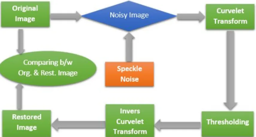
The proposed method consist of three parts, Curvelet transform(FDCT), Curvelet coefficients processing and inverse transform(IFDCT). In the first step Curvelet transform of noisy image is calculated which are thresholded by different thresholding function. Finally, inverse Curvelet transform is found to reconstruct denoising image. The reconstructed denoised image was com-pared with original image using SSIM, MSE, SNR and PSNR. An entropy-based thresholding [4, 5, 6] has been implemented in Curvelet domain for better result. The next modification can be use of clustering-based thresh-olding methods. Curvelet denoising technique is applied to any type of images like natural, satellite, medical like Computed Tomography (CT), Magnetic Resonance Imaging (MRI), Positron Emission Tomography (PET), Single Photon Emission Computed Tomography (SPECT), Ultrasonic images, etc.

1.2 Review of Literature

Many researchers, proposed various denoising technique like Wavelet based thresholding, Wiener ﬁltering etc. The Curvelet transform is a recently in-troduced as non-adaptive multi-scale transforms that is mainly popular in the image processing ﬁeld.

Kumar et al. [1] in 2010 proposed two filtering (Median and Wiener filters) algorithms to denoise image with different types of noise (Gaussian noise, Salt & Pepper noise and Speckle noise) that are either present in the image during capturing or injected into the image during transmission. Conclusion drawn from the paper was that, the performance of the Wiener filter after denoising for Speckle and Gaussian noisy image is better than Median filter. The performance of the Median filter after denoising for Salt & Pepper noisy

(15)

CHAPTER 1. INTRODUCTION 3 image is better than Wiener ﬁlter.

Candes et al. [2, 7] in 2006 describe the second generation Curvelet trans-form in two and three dimensions for image representation. They have intro-duced two methods for transformation as given, the ﬁrst digital transforma-tion is based on FDCT via unequally spaced fast fourier transforms, while the second is based on FDCT via wrapping. Those are diﬀered by spatial grid used for translate Curvelets at each scale and angle. However, wrapping is better than USFFT, because of the wrapping method take less computational time than USFFT.

Starck et al. [3] in 2002 presented a strategy for digitally implementing for both transforms the Ridgelet and the Curvelet. Both the transformation techniques have the property of exact reconstruction which is stable in nature. Huang et al. [8] in 2004 categorized a survey of image thresholding meth-ods. In this literature we have observed that the clustering-based method of Kittler and Illingworth [9] and the entropy-based methods of Kapur, Sahoo, and Wong [10], and Sahoo, Wilkins, and Yeager [11], are the best performing thresholding algorithms. Similarly, the clustering-based method of Kittler and Illingworth [9] and the local-based methods of Sauvola and Pietaksinen [12] and of White and Rohrer are the best performing document binarization algorithms. However, these results are obtained only from text document images degraded with noise and blur. For example, the increasing number of color documents becomes a new challenge for binarization and segmenta-tion. Multilevel thresholding, or simply multi-thresholding is gaining more applicability in vision applications. A few authors have addressed this issue in [13, 14, 15, 16, 17, 18, 19].

Sezginet al. [8] in 2004 describe diﬀerent image thresholding and compare between all thresholding technique. We have seen that authors are categorize the thresholding techniques in six group depend on there information. The categories are:

(16)

CHAPTER 1. INTRODUCTION 4 2. Entropy-based Thresholding

3. Clustering-based Thresholding

4. Attribute Similarity-based Thresholding

5. Spatial Thresholding

6. Local Adaptive Thresholding

Literature suggests entropy-based and clustering-based thresholding both are providing better performance compared to other technique.

Amani et al. [5] in 2009 describe entropy-based image thresholding for image segmentation. This approach is derived from ‘Pal method’ [4] that segment images using minimum cross-entropy thresholding based on Gamma distribution instead of Gaussian distribution. Gamma distribution has ability of representing symmetric and non-symmetric histograms. This proposed method is tested by using Synthetic Aperture Radar (SAR) images and it gives reliable results for bi-modal and multi-modal images. This method is more general than Pal [4] method and experimental results on SAR images showed good results in thresholding.

Osaimi et al. [6] in 2008 presents a new algorithm for SAR image seg-mentation based on thresholding technique. Generally, segseg-mentation of a SAR image falls under two categories; one based on grey levels and the other based on texture. This paper deals with SAR image segmentation based on grey levels and developed a new formula using Minimum Cross Entropy Thresholding (MCET) method for estimating optimal threshold value based on Gamma distribution to analyzing data of images; that means histogram of SAR images is assumed to be a mixture of Gamma distributions. It ap-plied on both bi-modal and multi-modal images. The contributions of this method include an iterative programming technique that is proposed for re-ducing huge computations. The experimental results obtained are promising

(17)

CHAPTER 1. INTRODUCTION 5 and it encourage future research for applying this method to complex image processing and computer vision problems and applications.

1.3 Motivations

Multiplicative noise or speckle noise occurred in various imaging systems due to random variation of pixel values. Although a number of restoration techniques were proposed in literature like Wiener ﬁltering and Lee ﬁltering to denoise such kind of noisy images, however these methods are not giving promising results in terms of PSNR, MSE and SNR. In this present research, we use various thresholding techniques like hard thresholding and entropy based thresholding in curvlet domain to denoise these images. The objective of this research is given as:

1.4 Objectives of the Thesis

The salient objectives of the thesis are:

• Reduce multiplicative noise in images using diﬀerent restoration tech-niques.

• Analysis of the denoising method in frequency domain using Wiener ﬁltering.

• Implementation of the proposed denoising method in transform domain using diﬀerent thresholding.

• Compared reconstructed image with original image using following sta-tistical parameters- SSIM, SNR, PSNR and MSE for diﬀerent noise vari-ance.

• Development of a real-time image processing system using Matlab GUI. 1.5 Thesis Organisation

(18)

CHAPTER 1. INTRODUCTION 6 • Chapter 1, Introduction.

• Chapter 2, Images under Multiplicative Noise. • Chapter 3, Multiplicative Noise.

• Chapter 4, Methodology of Image Denoising. • Chapter 5, Performance Assessment.

• Chapter 6, Result and Discussions.

• Chapter 7, concludes the thesis. Extensions of the present work and future scopes for further work are also discussed therein.

(19)

Chapter 2

IMAGES UNDER MULTIPLICATIVE

NOISE

2.1 Introduction

2.1.1 Synthetic Aperture Radar Image

Speckle is significant in Synthetic Aperture Radar (SAR) and Ultrasound imaging. SAR image is shown in figure: 2.1. Active Remote Sensing Satellite for earth observation capture two-dimensional (2-D) image. Range measure-ment and resolution are achieved in SAR in the same manner as most other radars: Range is determined by precisely measuring the time from transmis-sion of a pulse to receiving from a target in the wave length range 1mm to 1m of electromagnetic spectrum. The simplest SAR range resolution is de-termined by the transmitted pulse width, i.e. narrow pulses yield fine range resolution.

Since SARs are much lower in frequency than optical systems, even mod-erate SAR resolutions require an antenna physically larger than the practical size carried by an airborne platform usually hundred meters long antenna lengths are often required. However, airborne radar could collect data while ﬂying this distance and then process the data as if it came from a physically long antenna. The distance the aircraft ﬂies in synthesizing the antenna is known as the synthetic aperture. A narrow synthetic beam width resulting

(20)

CHAPTER 2. IMAGES UNDER MULTIPLICATIVE NOISE 8

Figure 2.1: SAR image

from the relatively long synthetic aperture, yields finer resolution than the resolution possible from a smaller physical antenna. Achieving fine azimuth resolution may also be described from a doppler processing viewpoint. A target’s position along the flight path determines the doppler frequency of its backscattering. Targets ahead of the aircraft produce a positive doppler offset, targets behind the aircraft produce a negative offset. The target’s doppler frequency determines its azimuth position. While this section at-tempts to provide an intuitive understanding, SARs are not as simple as described above. Transmitting short pulses to provide range resolution is generally not practical.

Applications of Synthetic Aperture Radar Imaging:

The application of SAR imaging is increased day by day due to the de-velopment of new technologies and innovative ideas.The areas, where this imaging technique used are given as:

• Reconnaissance, Surveillance, and Targeting • Treaty Veriﬁcation and Nonproliferation • Interferometry (3-D SAR)

• Navigation and Guidance

(21)

CHAPTER 2. IMAGES UNDER MULTIPLICATIVE NOISE 9 • Moving Target Indication

• Change Detection

• Environmental Monitoring

Speckle Noise in Satellite (SAR) Image

SAR is a coherent imaging technology that records both the amplitude and the phase of the back-scattered radiation as shown in figure: 2.2. An im-portant feature that degrades SAR images quality is speckle noise. Speckle is a common noise-liken phenomenon in all coherent imaging systems [20, 21]. Each resolution cell of the system contains many scatterers, the phases of the return signals from these scatterers are randomly distributed and speckle is due to the coherent nature of the sensor and the signal processing. The speckle noises will appear as bright or dark dots on the image and leads to limitation on the accuracy of the measurements given that the brightness of a pixel is determined not only by properties of the scatterers in the res-olution cell, but also by the phase relationships between the returns from those scatterers. Speckle noise is multiplicative in nature, therefore speckle reduction techniques is essential before procedures such as automatic target detection and recognition, thus traditional filtering will not remove it easily. Speckle noise prevents automatically target recognition and texture analysis algorithm to perform efficiently and gives the image a grainy appearance. Hence, speckle filtering turns out to be a critical pre-processing step for de-tection or classification optimization. Degraded image with speckle noise in SAR imaging is given by the equation;

d(X,Y) =I(X,Y)∗S(X,Y) (2.1) Where, d(X,Y) is the degraded ultrasound image with speckle, I (X,Y) is the original image and S(X,Y) is the speckle noise. Where (X,Y) denotes the pixel location. The multiplicative nature of speckle complicates the noise reduction process [22].

(22)

CHAPTER 2. IMAGES UNDER MULTIPLICATIVE NOISE 10

Figure 2.2: Complex case of microwave signal backscattering from multiple targets

2.1.2 Ultrasound Imaging

Introduction

It is a medical imaging technique that uses high frequency sound waves and their echoes. The technique is similar to the echolocation used by bats, whales and dolphins, as well as SONAR used by submarines. In ultrasound, the following events happen:

1. The ultrasound machine transmits high-frequency (1 to 5 megahertz) sound pulses into the human body using a probe.

2. The sound waves travel into the body and hit a boundary between tissues (e.g. between fluid and soft tissue, soft tissue and bone). Echoes are produced at any tissue interface where a change in acoustical impedance occurs. On these images, the film density is proportional to the intensity of the echo (a more energetic echo would produce a darker or lighter dot on the film). The intensity of the returning echo, that is the energy returned to the transducer, is determined by,

• The magnitude of the change in the acoustical impedance at the echoing interface.

(23)

CHAPTER 2. IMAGES UNDER MULTIPLICATIVE NOISE 11 • The normality (perpendicularity) of the interface to the transducer. • The appearance of the echo on the ﬁlm is also determined by the degree of ampliﬁcation (gain) applied after the echo has been received by the transducer.

3. Hence some of the sound waves get reﬂected back to the probe, while some travel on further until they reach another boundary and get re-ﬂected.

4. The reﬂected waves are picked up by the probe and relayed to the ma-chine.

5. The machine calculates the distance from the probe to the tissue or organ (boundaries) using the speed of sound in tissue (1,540 m/s) and the time of the each echo’s return (usually on the order of millionths of a second).

6. The machine displays the distances and intensities of the echoes on the screen, forming a two dimensional image.

These scans use high frequency sound waves which are emitted from a probe. The echoes that bounce back from structures in the body are shown on a screen as shown in ﬁgure: 2.3. The structures can be much more clearly seen when moving the probe over the body and watching the image on the screen. The main problem in these scans is the presence of speckle noise which reduces the diagnosis ability.

(24)

CHAPTER 2. IMAGES UNDER MULTIPLICATIVE NOISE 12 Applications of Ultrasound Imaging

Ultrasound has been used in a diﬀerent types of clinical settings, like ob-stetrics, gynecology, cardiology and in cancer detection. The main advantage of ultrasound is that certain structures can be observed without using radia-tion. Ultrasound is more faster than X-rays or other radiographic techniques. Here some applications of ultrasound in medical imaging system is describe below:

1. Obstetrics and Gynecology

2. Cardiology

3. Urology

In addition to these areas, there is a growing use for ultrasound as a rapid imaging tool for diagnosis in emergency rooms.

Speckle Noise in Ultrasound Image

Ultrasound imaging being inexpensive, nonradioactive, real-time and non-invasive, is most widely used in medical ﬁeld. To achieve the best possible diagnosis it is important that medical images be sharp, clear and free of noise and artifacts[23]. However occurrence of speckle is a problem with ultrasound imaging. Speckle is the artifact caused by interference of energy from ran-domly distributed scattering [24, 25, 26, 27]. Speckle noise tends to reduce image resolution and contrast and blur important details, thereby reducing diagnostic value of this imaging modality. Therefore speckle noise reduction is an important prerequisite whenever ultrasound imaging is used. Denoising of ultrasound images however still remains a challenge because noise removal causes blurring of the ultrasound images. Sometimes physicians prefer to use original noisy images rather than ﬁltered ones because of loss of important features while denoising. Thus appropriate method for speckle suppression is needed which enhances the signal to noise ratio while conserving the edges and lines in images.

(25)

CHAPTER 2. IMAGES UNDER MULTIPLICATIVE NOISE 13 Speckle is generally considered to be multiplicative in nature. Within each resolution cell a number of elementary scatterers reﬂect the incident wave towards sensor. The backscattered coherent waves with diﬀerent phases undergo a constructive or a destructive interference in a random manner. The acquired image is thus corrupted by a random granular pattern, called speckle that delays the interpretation of the image content.

2.2 Chapter Summary

This chapter, discussed basic imaging systems which includes deﬁnition of image, type of imaging and there deﬁnition with application. The types of imaging requires capturing device like sensor and circuitry of scanner or digital camera, these image capturing device add extra information which is also called as noise. Noise is undesirable signal which is a random variation of brightness or color information in an image. There are various types of such noise which have been described in Chapter: 3.

(26)

Chapter 3

MULTIPLICATIVE NOISE

Image Noise is random variation of brightness or color in an image. It can be produced by any circuitry such as sensor, scanner or digital camera. Image noise is an undesirable signal, it’s produce by image capturing device that add extra information. In many cases, it reduces image quality and is especially signiﬁcant when the objects being imaged are small and have relatively low contrast. This random variation in image brightness is designated noise. This noise can be either image dependent or image independent.

3.2 Speckle Noise

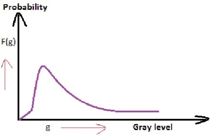
Speckle noise is multiplicative noise. This type of noise occurs in various imaging systems such as Laser, Medical, Optical and SAR imagery. The source of this noise is a form of multiplicative noise in which the intensity values of the pixels in the image are multiplied by random values. Speckle noise in image is serious issue, causing diﬃculties for image representation. It is caused by coherent processing of backscattered signals from multiple distributed targets. The fully developed speckle noise has the characteristic of multiplicative noise. Speckle noise in image is a multiplicative noise, it is in direct proportion to the local grey level in any area.

(27)

CHAPTER 3. MULTIPLICATIVE NOISE 15

P (x,y) =a(x,y)·b(x,y) (3.1) Here a(x,y) is original signal and b(x,y) is noise introduce into signal to produce the corrupted image P (x,y). (x,y) represent the pixel location. Speckle noise follows a gamma distribution and it is give by:

F (g) = g

α−1

(α−1) !aαe

−g

a (3.2)

Where, aα is variance, g is gray level and F (g) is Gamma distribution. The ﬁgure 3.1 below shows the plot of speckle noise gamma distribution.

Figure 3.1: Probability density function of speckle noise model

It arises from random variations in the strength of the backscattered waves from objects and is seen mostly in RADAR and Ultrasound imaging.

Statistics of Speckle Noise

The pixel-to-pixel intensity variation in SAR images has a number of con-sequences; the most obvious one being that the use of a single pixel intensity value as a measure of distributed targets’ reﬂectivity would be erroneous [22]. We know that the received signal is complex; let r and i denote its real and imaginary components. For a single-look SAR image, the intensity I=r2+i2

of a zone of constant reﬂectivity is exponentially distributed. The amplitude A, which is the square root of I, follows a Rayleigh distribution. For an

(28)

CHAPTER 3. MULTIPLICATIVE NOISE 16 N-look image and independent looks, the intensity follows a Gamma distri-bution. There are several ways of obtaining N-look amplitude images in the spatial domain:

Case 1. Averaging N amplitude images;

Case 2. Averaging N intensity images, then taking the square root;

Case 3. Coherently averaging complex images by means of the Weighted Filter [23], then taking the square root.

In case 1, the probability density function is obtained by N convolutions of Rayleigh distributions, but cannot be expressed in analytic form. In the cases 2 and 3 it can be shown that the amplitude follows a K -distribution.

A usual way of characterizing the speckle level in SAR image is to compute

L=E2(I)/σ2(I) over an area of constant reﬂectivity; L is often called ENIL (Equivalent Number of Independent Looks) and gives no information on the spatial resolution of an image. We will also use the MSE between the ideal and noisy images (in the case where the ideal image is available), which reﬂects both speckle reduction and preservation of structures.

Model of Speckle Noise

An inherent characteristic of ultrasound imaging is the presence of speckle noise. Speckle noise is a random and deterministic in an image. Speckle has negative impact on ultrasound imaging, Radical reduction in contrast resolution may be responsible for the poor eﬀective resolution of ultrasound as compared to MRI. In case of medical literatures, speckle noise is also known as texture. Generalized model of the speckle is represented as,

g(n,m) =f (n,m)∗u(n,m) +ξ(n,m) (3.3) Where, g(n,m) is the observed image, u(n,m) is the multiplicative com-ponent and ξ(n,m) is the additive component of the speckle noise. Here n and m denotes the axial and lateral indices of the image samples. In the ultrasound imaging consider only multiplicative noise and additive noise is

(29)

CHAPTER 3. MULTIPLICATIVE NOISE 17 to be ignored. Hence, above equation can be modiﬁed as;

Therefore,

g(n,m) =f (n,m)∗u(n,m) +ξ(n,m)−ξ(n,m)

g(n,m) =f (n,m)∗u(n,m) (3.4) 3.3 Image with Diﬀerent Types Noise

Quality of an image is degraded by noise. Various type of noise can come into image with different strength. Some noisy images with different level of variance is shown in figure: 3.3.

(a) (b)

(c) (d)

Figure 3.2: (a) Original SAR image, (b) Gaussian noisy SAR image with var. 0.02, (c) Salt and Pepper noisy SAR image with var. 0.05, (d) Speckle noisy SAR image with var. 0.08

3.4 Chapter Summary

This chapter, discussed noise in image which includes deﬁnition of noise, char-acteristics and major causes. The types of imaging requires capturing device like sensor and circuitry of scanner or digital camera, these image capturing device add extra information which is also called as noise. Noise is undesir-able signal which is a random variation of brightness or color information in

(30)

CHAPTER 3. MULTIPLICATIVE NOISE 18 an image. After addition of noise in an image, the image quality is degrades. So, removing noise from images ﬁrst we analyse a restoration technique in fre-quency domain after proposed a restoration techniques in sparse domain for better vision. There are restoration techniques which can used for denoising the multiplicative noisy image have been described in Chapter: 4.

(31)

Chapter 4

METHODOLOGY OF IMAGE

DENOISING

Image denoising is one of the most essential task in image processing. Two diﬀerent technique of image restoration can be used for image denois-ing. These are Wiener ﬁltering and various thresholding in Curvelet domain. Using some statistical parameter such as SSIM, MSE, SNR, PSNR we can calculate the amount of information retained in the denoising image compare to original image.

4.2 Simulation of Noisy Image

Synthetic Aperture Radar images have been taken from NASA (National Aeronautics and Space Administration) and ESA (European Space Agency). Here, We used satellite imagery (SAR) and standard image (Lena) for test-ing of different restoration techniques. These images are corrupted with uni-formly distributed multiplicative noise having different levels of variance of the noise. By taking four different values of noise variances, four different SAR noisy images are being obtained. The range of noise variance are [0.04 0.08], where the variance 0.04 represents low level noisy image and variance 0.08 represents a high level noisy image.

(32)

CHAPTER 4. METHODOLOGY OF IMAGE DENOISING 20 4.3 Image Denoising Methods

This chapter we focus on two diﬀerent techniques of image restoration, one is exiting Wiener ﬁltering for analyses of denoising and other one is proposed in Curvelet domain with various thresholding [4, 5, 6, 28].

4.3.1 Image Denoising in Frequency Domain

For analyses the restoration process using Wiener ﬁltering denoising the image when it is corrupted by speckle noise [1] with diﬀerent variance.

Techniques Used for Image Denoising

• Wiener ﬁltering

• Estimation of statistical parameters Wiener Filtering

Wiener filter is a optimum linear filter which is involved only for linear estimation of a desired signal sequence. In the statistical approach to the solution of the Wiener filtering problem, we assume the statistical parameters of the useful signal and unwanted additive noise. The Wiener filter algorithm considers a signalSx(f) corrupted with noiseSn(f). The noise has zero mean

and variance of σ_n2. The resulting signal obtained after Wiener ﬁltering be

H (f). The transfer function corresponding to Wiener ﬁlter was given by:

H (f) = Sxy(f)

Sy(f)

= Sx(f)

Sx(f) +Sn(f)

(4.1)

This filter-optimization problem is to minimize the mean-square error of the signal that is defined by the actual filter output. This resulting solution is commonly known as the Wiener filter. The block diagram of a Wiener filter is shown in figure: 4.1,

(33)

CHAPTER 4. METHODOLOGY OF IMAGE DENOISING 21

Figure 4.1: Block Diagram of Wiener Filtering to Denoise The Speckle Im-age. Here, G(Z) = N ∑ i=0 aiZ−i

w[n] and s[n] are random process signal. The filter output is x[n] and e[n] are the estimation error. An input signal w[n] is convolved with the Wiener filter G[z] and the result is compared to a reference signal s[n] to obtain the filtering error e[n]. The image denoising using the Wiener filter is shown in the flowchart in figure 2.2.

Figure 4.2: Flowchart of denoising algorithm using Wiener ﬁltering.

Wiener Filter Characterization

(34)

CHAPTER 4. METHODOLOGY OF IMAGE DENOISING 22 1. Assumption: signal and additive noise are casual processes with known spectral characteristics or known autocorrelation and cross-correlation.

2. Requirement: the ﬁlter must be physically realizable/causal.

3. Performance criteria: minimum mean-square error (MMSE).

This ﬁlter is frequently used in the process of deconvolution on the pixel of image using ﬁltering window mask.

Advantage and Drawback of Wiener Filtering The wiener ﬁlter expression is,

G(x, y) = H ∗₍_{x, y}₎ |H (x, y)|2 + Sn(x,y) Sf(x,y) G(x, y) = H ∗₍_{x, y}₎_×_S f (x, y) |H(x, y)|2 ×Sf (x, y) +Sn(x, y) (4.2) Here, • H (x, y) = Degradation Function.

• H∗(x, y) = Complex Conjugate of Degradation Function. • Sn(x, y) = Power Spectral Density of Noise.

• Sf (x, y) = Power Spectral Density of Un-degraded Image.

Wiener filter is better for noise reduction because it uses statistical knowledge of the noise field. The transfer function of the Wiener filter is chosen to minimize the mean square error using statistical information on both image and noise field. The choice of window size of Wiener filter depends upon the noise variance of image.

(35)

CHAPTER 4. METHODOLOGY OF IMAGE DENOISING 23 Algorithm of Image Denoising Using Wiener Filtering

Here, we analyse an algorithm based on Wiener ﬁltering for image denois-ing usdenois-ing logarithmic transformation.

1. Algorithm for denoising using Wiener filter:

Step 1: Take an original image.

Step 2: Add diﬀerent variance of multiplicative(speckle) noise with orig-inal image.

Step 3: Convert the multiplicative noisy image into additive noisy image using logarithmic transformation.

Step 4: Applying the Wiener filtering to additive noisy image. Here, we using different size of Wiener filter mask. The mask size depending upon noise variance.

Step 5: Showing the restored image after Wiener ﬁltering.

Step 6: Convert the restored image from additive to multiplicative form using anti-logarithmic transformation.

Step 7: Compare the restored image that obtained in step 6 with original image and estimate various statistical parameters like SSIM, SNR, MSE and PSNR, etc.

4.3.2 Image Denoising in Sparse/Transform Domain

After analyse wiener ﬁltering, we proposed a restoration technique in sparse/transform domain using diﬀerent thresholding techniques with logarithm or without

log-arithm for denoising the image [29, 3] with diﬀerent noise variance.

Techniques Used for Image Denoising

• Curvelet Transform • Thresholding

(36)

CHAPTER 4. METHODOLOGY OF IMAGE DENOISING 24 Curvelet Transform

Curvelet transform was introduced by E. J. Candes [2]. On theoretical basis they are introduced two methods for transformation as given below:

• Unequispaced FFT Transform • Wrapping Transform

Those are diﬀer by spatial grid used for translate Curvelets at each scale and angle. However, wrapping algorithm provide faster computational technique or take less time than USFFT.

The idea of the Curvelet transform is ﬁrst to decompose the image into Subband. The discrete Curvelet transform is mathematically expressed as:

cD(j, l, k) = ∑

0≤t1,t2<n

f [t1, t2]φD_j,l,k[t1, t2] (4.3)

Where, f [t1, t2] is 2D signal of cartesian arrays with t1 ≥ 0 and t2 < n.

CD(j, l, k) are Curvelet coeﬃcients at scale j, location l and coordinates k = (k1,k2) ∈ Z2, and φDj,l,k is a digital Curvelet waveform, here the superscript D

is stands for digital. For detail follow in [2].

Advantage and Drawback of Curvelet Transform The advantage of using curvelet are,

1. Curvelet approximate line singularity better than other transformation,

2. It is an optimal representation with edges.

The main drawback of the Curvelet transform is redundancy factor. It is redundant with a factor equal to J+1 for J scales.

Algorithm of Image Denoising in Curvelet Domain

Here, we proposed two diﬀerent algorithm in Curvelet domain with two dif-ferent thresholding methods like hard-thresholding and MCET thresholding

(37)

CHAPTER 4. METHODOLOGY OF IMAGE DENOISING 25 for image denoising, ﬁrst algorithm is for image denoising in Curvelet domain using hard thresholding without logarithmic function and second one is with logarithmic function.

Figure 4.3: Flowchart of Curvelet transform algorithm for image denoising using hard-thresholding.

1. Algorithm for denoising in Curvelet domain using Hard thresh-olding:

Step 1: Take the original image.

Step 3: Apply the Curvelet transformation of noisy image.

Step 4: Apply diﬀerent thresholding approach over the Curvelet coeﬃ-cient.

Step 5: Applying inverse Curvelet transformation to obtain the restored image over the thresholded Curvelet coeﬃcient.

Step 6: Calculate the information retained in the denoised image using statistical indices such as SSIM, SNR, MSE and PSNR.

1. Algorithm for denoising in Curvelet domain using Hard thresh-olding with Logarithm function:

(38)

Figure 4.4: Flowchart of Curvelet transform algorithm for image denoising using hard-thresholding with logarithm.

Step 1: Take the original image.

Step 3: Convert the multiplicative noisy image into additive noisy image using logarithmic transformation.

Step 4: Apply the Curvelet transformation on noisy image.

Step 5: Apply diﬀerent thresholding approach over the Curvelet coeﬃ-cient.

Step 6: Applying inverse Curvelet transformation to obtain the restored image over the thresholded Curvelet coeﬃcient.

Step 7: Convert the restored image from additive to multiplicative form using anti-logarithmic transformation.

Step 8: Calculate the information retained in the denoised image using statistical indices such as SSIM, SNR, MSE and PSNR.

(39)

4.3.3 Image Thresholding

Thresholding is one of the most effective technique for image segmentation. It is a non-linear operation that converts a binary image from a gray-scale image. Where the two levels are assigned for pixels that are below or above the specified threshold value. In many applications, it is useful to separate out the regions of the image corresponding to objects and background in which we want to analyze. Thresholding often provides an easy and convenient way to perform this segmentation on the basis of the different intensities or colors in the foreground and background regions of an image.

Why to Use Thresholding?

• The simplest segmentation method.

• Separate out regions of an image to objects which we want to analyze. This separation is based on the variation of intensity between the object pixels and the background pixels.

How to Select Threshold Value

A gray scale image and its corresponding histogram are shown below:

(a) (b)

Figure 4.5: (a) Gray scale SAR image, (b) Histogram of corresponding gray scale SAR image Looking at the picture ﬁgure: 4.5 on left, there are no white pixel value(255) and we can see that the histogram with this observation. So, select an

(40)

accu-CHAPTER 4. METHODOLOGY OF IMAGE DENOISING 28 rate threshold value from the histogram above that the most dominate (high to peak value of histogram) pixel value. So, if we select threshold value of ‘40’, then every pixel value below the threshold is black and above the threshold is white. After the threshold we will get the following binary image.

Figure 4.6: Binary image of corresponding gray seal image.

Types of Thresholding

Diﬀerent types of thresholding are used for denoising image. Threshold can be chosen by manually and automatically. It can be categorized into two groups, global and local threshold. Global thresholding technique, thresholds the complete image with a single threshold value and in local thresholding technique, segment the image into a number of sub-image and use a diﬀer-ent threshold value for each sub-image. Global thresholding methods are easy to implement and faster because it take less computational time. Basic thresholding methods which is use for image segmentation these are:

i. Automatical calculation of threshold value using an iterative method.

ii. Hard Thresholding.

iii. Soft Thresholding.

iv. Adaptive Thresholding.

v. Approximate the histogram of the image and choose a mid-point value of histogram as the threshold level.

(41)

CHAPTER 4. METHODOLOGY OF IMAGE DENOISING 29 In [8] thresholding methods are categorized in six diﬀerent groups depends on the information they are exploiting. These categories are:

a. Histogram shape-based methods.

b. Clustering-based methods.

c. Entropy-based methods.

d. Objective attribute-based methods.

e. Spatial information-based methods.

e. Local adaptive methods.

We derived the two diﬀerent methods of thresholding like hard threshold-ing and entropy-based thresholdthreshold-ing usthreshold-ing for image denoisthreshold-ing.

Hard Thresholding

Hard-thresholding is a type of global thresholding, in this thresholding method thresholds the complete image with a single threshold value. So using that method for image denoising select one threshold value for whole image. Hard thresholding sets to zero those element whose absolute value is lower than the threshold value and neglecting zero element. Hard thresholding function is as follows:

f(y)= {

y,|y|>λ

0,|y| ≤ λ (4.4)

Where, y and f(y) are the Curvelet coeﬃcients before and after hard threshold processing, λ is a threshold value.

Entropy-based Thresholding

Entropy is measure of the uncertainty in a random variable. Image entropy is a quantity which is used to describe the amount of information retained in an image. The entropy or average information of an image can be determined

(42)

CHAPTER 4. METHODOLOGY OF IMAGE DENOISING 30 approximately from the histogram of the image. The histogram shows the diﬀerent gray level probability in the image [30, 31].

Entropy Thresholding

Entropy thresholding is a means of thresholding an image that selects an optimum threshold value by choosing the pixel intensity from image his-togram that show the maximum entropy over the entire image [10, 32, 33].

Type of Entropy Thresholding 1. Entropic Thresholding.

2. Cross-entropic Thresholding.

3. Fuzzy-entropic Thresholding.

Cross-entropic Thresholding

Cross entropy is a type of information theoretic distance between two probability distribution, it also known as divergence or cross-entropy [28, 4, 6].

Let, two probability distributionP = (P1, P2...Pn) andQ= (Q1, Q2...Qn).

So, Cross-entropy deﬁne,

For symmetric version can be written as:

DS (P, Q) = S ∑ i=1 pilog pi qi + L ∑ i=S+1 qilog qi pi (4.5)

For asymmetric version can be written as:

DS(P, Q) = S ∑ i=1 pilog pi qi (4.6) where, 1. i is gray-level(1,2,...L) value.

(43)

CHAPTER 4. METHODOLOGY OF IMAGE DENOISING 31 2. Pi is probability of occurrence of gray-level.

3. pi = _Mh_×i_N

4. hi is frequency of gray-level.

Assumed threshold S partitions the image into two regions, object and background. Let, S assume the the gray value(0 to S) assigned for object and ((S+1) to L) assigned for background. Now describe the cross-entropy of segmented image with threshold S,

D(S) = S ∑ i=1 ihilog i µ1(S) + L ∑ i=S+1 ihilog i µ2(S) (4.7)

where, Average intensity value of foreground,

µ1(S) = ∑S i=1(ihi) ∑S i=1hi (4.8)

Average intensity value of background,

µ2(S) = ∑L i=S+1(ihi) ∑L i=S+1hi (4.9) 4.4 Chapter Summary

This chapter discusses various restoration techniques of multiplicative noisy image. The restoration is done by Wiener filtering in frequency domain. The restored image may be blurred if the windows size of Wiener filter is large. This means that part of information a true image has also been loss along with noise. These mask size of Wiener filter are varied depending upon the presence of noise variance in an image. The advantages and drawbacks of Wiener filtering are describe in section 4.3.1.

To overcome this drawback, a novel image denoising algorithm in sparse/ transform domain using diﬀerent thresholding techniques has been proposed. The performance of the algorithm can be judged using SSIM, MSE, SNR, PSNR. These parameters have been described in Chapter: 5.

(44)

Chapter 5

PERFORMANCE ASSESSMENT

The parameters which are used in the ﬁlter performance evaluation are Signal to Noise Ratio (SNR), Mean Square Error (MSE), Peak Signal to Noise Ratio (PSNR) and Structural Similarity Index Measure (SSIM) [34, 35].

5.1.1 Measurement of SNR

Signal-to-noise ratio (SNR or S/N) is deﬁned as signal power to noise power of the corrupting signal. It is one of the most essential statistical parameter for quality measurement of an image or signal. When a ratio higher than 1:1 then it is indicates more signal power than noise power, it guarantees lower distortion and less interference cause by presence of noise. It can be derived from the formula,

SN R=Psignal

Pnoise

(5.1)

where, Psignal is the signal mean or expected value and Pnoise is the

stan-dard deviation of the noise.

5.1.2 Measurement of MSE

MSE is deﬁne as the average of square of the error. Where error is the diﬀeren between desire quantity and estimated quantity. The MSE provides a means of choosing the best estimator. We also calculate Root Mean Square

(45)

CHAPTER 5. PERFORMANCE ASSESSMENT 33 Deviation taking the square root of MSE, it is also good statistic parameter for measure quality of image. Having a Mean Square Error of zero (0) is ideal. The MSE is deﬁned as:

M SE= N ∑ i=j=1 [f (i,j)−F (i,j)]2/N2 (5.2) 5.1.3 Measurement of PSNR

The Peak Signal-to-Noise Ratio (PSNR) [36] is define as a ratio between the maximum possible power of a signal and the noise power that affects the fidelity of its representation. PSNR is usually expressed in terms of the logarithmic decibel scale. The PSNR is most commonly used as a measure of quality of reconstruction of lossy compression for image compression. It is most easily defined via the mean squared error (MSE) which for two m×n

monochrome images I and K where one of the images is considered a noisy approximation of the other is deﬁned as:

M SE=

N

∑

i=j=1

[f (i,j)−F (i,j)]2/N2

The PSNR is deﬁned as:

P SN R=10log₁₀(M AX2_I

M SE ) =20log10( M AXI

M SE ) (5.3)

Here,M AXI is the maximum possible pixel value of the image. When the

pixels are represented using 8 bits per sample, this is 255. More generally, when samples are represented using linear PCM with B bits per sample,

M AXI is 2B −1.

5.1.4 Measurement of SSIM

The SSIM is an index that measure the similarity between two images. Recently the SSIM approach for image quality assessment [36]. The SSIM is

(46)

CHAPTER 5. PERFORMANCE ASSESSMENT 34 calculated on various windows of an image. Let, the measure between two windows f and g. This window is common size metric N×N.

SSIM (f ,g) =l(f ,g)α·c(f ,g)β·s(f ,g)γ Where, α>0, β>0, γ>0 SSIM (f, g) = ( (2µfµg + c1) (2σfσg +c2) µ2_f + µ2 g + c1 ) ( σ_f2 +σ2 g +c2 ) (5.4) Where, • µf = The average of f. • µg = The average of g. • σ_f2 = The Variance of f. • σ_g2 = The Variance of g.

• σ_{f g} = The Covariance of f and g • c1 = (k1, L)

2

and c2 = (k2, L) 2

two variables that stabilize the division with weak denominator.

• L is the dynamic range of pixel value and k1 = 0.01 and k2 = 0.03 by

default value.

We can also measured some image quality assessment such as MSSIM (Mean Structural Similarity Index), UQI (Universal image Quality Index) [37], SS-SSIM (Single-Scale Structural Similarity Index), MS-SSIM (Multi-Scale Structural Similarity Index), MAE (Mean Absolute Error), RMS (Root Mean Squared Error), NCC (Non-linear regression Correlation Coeﬃcient), ROCC (Spearman Rank-Order Correlation Coeﬃcient), OR (Outlier Ratio), STD (Standard Deviation(σ)) between restored image and original image for compressions [34].

(47)

CHAPTER 5. PERFORMANCE ASSESSMENT 35 5.2 Chapter Summary

This chapter discussed various statistical parameters and quality performance measuring index for measuring quality of an images. These parameters can used for quality measurement and statistical information between original image and restored image after diﬀerent restoration techniques. The results of all restoration techniques have been described in Chapter: 6.

(48)

Chapter 6

RESULT & DISCUSSIONS

In this chapter, results of two diﬀerent image restoration techniques are pre-sented. First one is analysis of Wiener ﬁlter based method and the second one is proposed method in sparse/ transform domain using hard threshold-ing with and without logarithm function. The statistical parameters are computed for original and restored as well as original and noisy images. A comparative result is presented

(49)

CHAPTER 6. RESULT & DISCUSSIONS 37

6.1.1 Original Image with Diﬀerent Noise Variance

Original Image with Diﬀerent Noise Variance for Standard Image(Lena)

(a) (b) (c) (d)

Figure 6.1: (a) Original image, 512 by 512, 8bits/pixel,with MSE = 0, PSNR = ∞, (b) Speckle noisy image with var. 0.04, (c) Speckle noisy image with var. 0.06, (d) Speckle noisy image with var. 0.08

Original Image with Diﬀerent Noise Variance for Satellite Imagery(SAR)

(a) (b) (c) (d)

Figure 6.2: (a) Original image, 600 by 800, 8bits/pixel,with MSE = 0, PSNR = ∞, (b) Speckle noisy image with var. 0.04, (c) Speckle noisy image with var. 0.06, (d) Speckle noisy image with var. 0.08

(50)

6.1.2 Experimental Results of Denoising Image in Frequency Domain using Wiener Filter

Denoised Standard Image(Lena) in Frequency Domain using Wiener Filtering with Diﬀerent Noise Variance

(a) (b) (c) (d)

Figure 6.3: (a) Original image, 512 by 512, 8bits/pixel,with MSE = 0, PSNR = ∞, (b) Restored image of noise var. 0.04, (c) Restored image of noise var. 0.06, (d) Restored image of noise var. 0.08

Denoised Satellite Imagery(SAR) in Frequency Domain using Wiener Fil-tering with Diﬀerent Noise Variance

(a) (b) (c) (d)

(51)

CHAPTER 6. RESULT & DISCUSSIONS 39 For Standard Image(Lena)

Table 6.1: Comparison between original, noisy and restored image of Wiener ﬁltering with diﬀerent noise variance

Noise Statistical OriginalImage OriginalImage

Variance Parameter V s V s

Indices N oisyImage RestorImage

SSIM 0.6082 0.8340 0.04 MSE 687.8208 129.9290 SNR 3.1938 6.7864 PSNR 19.7900 27.0277 SSIM 0.5440 0.8097 0.06 MSE 1013.4 158.7002 SNR 2.7654 15.9708 PSNR 18.1069 26.1590 SSIM 0.5015 0.7879 0.08 MSE 1327.4 192.2015 SNR 2.5371 5.8259 PSNR 16.9347 25.3272

For Satellite Imagery(SAR)

Table 6.2: Comparison between original, noisy and restored image of Wiener ﬁltering with diﬀerent noise variance

(52)

(53)

6.1.3 Experimental Results of Denoising Image in Sparse/Transform Domain

Experimental Results of Denoising Image in Sparse/Transform Domain without Logarithm

Denoised Standard Image(Lena) in Sparse/Transform Domain with Diﬀerent Noise Variance using Hard-thresholding

(a) (b) (c) (d)

Figure 6.6: (a) Original image, 256 by 256, 8bits/pixel,with MSE = 0, PSNR = ∞, (b) Restored image of noise var. 0.04, (c) Restored image of noise var. 0.06, (d) Restored image of noise var. 0.08

Denoised Satellite Imagery(SAR) in Sparse/Transform Domain with Dif-ferent Noise Variance using Hard-thresholding

(a) (b) (c) (d)

(54)

CHAPTER 6. RESULT & DISCUSSIONS 42 For Standard Image(Lena)

Table 6.3: Comparison between original, noisy and restored image of Sparse/Transform domain using Hard-thresholding; with diﬀerent noise vari-ance

For Satellite Imagery(SAR)

Table 6.4: Comparison between original, noisy and restored image of Sparse/Transform domain using Hard-thresholding; with diﬀerent noise vari-ance

Variance Parameters V s V s

(55)

(56)

CHAPTER 6. RESULT & DISCUSSIONS 44 Experimental Results of Denoising Image in Sparse/Transform Domain with Logarithm

Denoised Standard Image(Lena) in Sparse/Transform Domain with Diﬀerent Noise Variance using Hard-thresholding with Logarithm

(a) (b) (c) (d)

Denoised Satellite Imagery(SAR) in Sparse/Transform Domain with Dif-ferent Noise Variance using Hard-thresholding with Logarithm

(a) (b) (c) (d)

Figure 6.10: (a) Original image, 600 by 800, 8bits/pixel,with MSE = 0, PSNR =∞, (b) Restored image of noise var. 0.04, (c) Restored image of noise var. 0.06, (d) Restored image of noise var. 0.08

(57)

CHAPTER 6. RESULT & DISCUSSIONS 45 Result of Hard-Thresholding with Logarithm For Standard Image(Lena)

Table 6.5: Comparison between original, noisy and restored image of Sparse/Transform domain using Hard-thresholding and logarithm function; with diﬀerent noise variance

Result of Hard-Thresholding with Logarithm For Satellite Imagery(SAR)

Table 6.6: Comparison between original, noisy and restored image of Sparse/Transform domain using Hard-thresholding and logarithm function; with diﬀerent noise variance

Variance Parameters V s V s

(58)

Figure 6.11: Statistical parameters Vs noise variance of sparse domain using hard-thresholding with logarithm

(59)

CHAPTER 6. RESULT & DISCUSSIONS 47 Denoised Bi-modal Image in Sparse/Transform Domain using MCET-thresholding

(a) (b) (c) (d)

Figure 6.12: (a) Original image, 256 by 256, 8bits/pixel,with MSE = 0, PSNR =∞, (b) Restored image of noise var. 0.04, (c) Restored image of noise var. 0.06, (d) Restored image of noise var. 0.08

For Bi-modal Image

Table 6.7: Comparison between original, noisy and restored image of Sparse/Transform domain using MCET-thresholding

SSIM 0.5490 0.7461 0.08 MSE 866.5108 813.6410

SNR 3.2218 3.8457 PSNR 18.7871 19.0605

(60)

CHAPTER 6. RESULT & DISCUSSIONS 48 6.2 Chapter Summary

In this chapter, the results of all restoration techniques such as the non-linear Wiener ﬁltering method in Frequency domain, Hard-thresholding in Sparse domain without logarithm and Hard-thresholding in sparse domain with logarithm have been described. The obtained restored image is com-pared with original image using some quantifying statistical parameters such as SSIM, MSE, SNR, PSNR to measure the performance index. So we con-clude that the restoration method Hard-thresholding in Sparse domain using logarithm is better than other nonlinear Wiener ﬁltering in Frequency do-main and Hard-thresholding in sparse dodo-main without logarithm methods. The resulted denoised image using hard thresholding in Curvelet domain with logarithm function provides 80% of performance measuring index (SSIM=0.8) with noise variance 0.08. Where, SSIM varies in between 0 to 1. SSIM 0 in-dicate noisy image and 1 inin-dicate noise free image. So, for getting SSIM close to 1, applying entropy-based thresholding methods in sparse domain and observed that this restoration technique works on only bi-modal images but not getting promising result of statistical parameters and quality per-formance measuring index. The results of this thesis may show important directions for further scope of research. The conclusion and further scope of research of this work have been described in Chapter: 7.

(61)

Chapter 7

CONCLUSION AND FUTURE SCOPE

In this thesis an attempt has been made to develop denoising methods for images under multiplicative noise.The performance of this method is evalu-ated and compared with that of existing state-of-the-art. In the ﬁrst section of this chapter an overview of contributions of the thesis and the conclusions are summarized. Topics for future research are pointed out in the second section of this chapter.

7.1 Conclusion

The multiplicative noise are often found to model the real time noise in several images like SAR, Ultrasound image etc. This thesis aims at developing a denoising method under multiplicative noise corruption. A Curvelet domain based approach with different thresholding technique has been developed. The thresholding on Curvelet coefficient is determine by an hard and entropy based thresholding method developed in [8]. The algorithm is applied to several standard images and performance is evaluated using statistical indices like SSIM, MSE, SNR, PSNR. Experimental results exhibits improvement over the exiting stat-of-art fordenoising such as Wiener filtering.