University of the Basque Country (UPV/EHU)
Master in Economics: Empirical Applications and Policies
Fiscal Policy Asymmetries and the Sustainability of Government Debt in the
Euro Area
Author: Bayram Bahadir Karaca1 Supervisors: Idoia Aguirre, Jesús Vázquez
July 2020
Abstract
This paper empirically analyzes fiscal policy sustainability and the cyclicality in 19 Euro Area countries using data on government debt, primary deficit and the output gap. We investigate this over quarterly intervals, which begin in 1980:1 and end in 2019:3. We find that primary deficit/GDP ratio responds negatively to an increase in government debt in weak economic times, which we interpret as sustainable fiscal policy in the economic times of distress. The best fitting threshold model and the Markov switching model do not support fiscal policy sustainability during economic expansions. Hence, we interpret the robust sustainable results during times of distress as evidence that policy makers are concerned with the fiscal rules and targets in weak economic times. Regarding the cyclicality of fiscal policy, we find symmetric and counter-cyclical behavior for Markov switching model.
Keywords: Fiscal policy sustainability, Fiscal policy asymmetry, Markov switching models, Threshold regression models
1
1
Contents
1. Introduction ... 2
2. EU Perspective ... 5
2.1 Fiscal Policy ... 5
2.2 Evolution of Macroeconomic Parameters ... 6
3. Methodology ... 8 3.1 Bohn’s Contributions ... 8 3.2 Empirical equations ... 10 3.3 Data ... 12 4. Results ... 13 5. Conclusions ... 19 6. References ... 20 7. Appendix ... 22
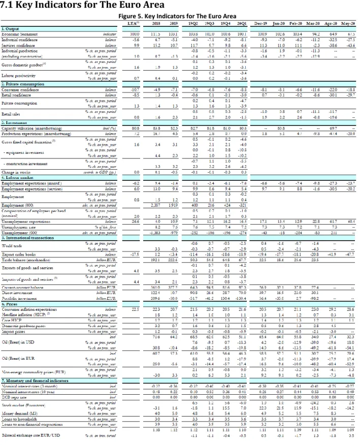
7.1 Key Indicators for The Euro Area ... 22
7.2 Likelihood Ratio Test Results ... 23
2
1. Introduction
Many economists and corporations do not agree on a unique definition of fiscal sustainability, rather, they have different but similar explanations. For example, OECD defines fiscal sustainability as the ability of a government to maintain public finances at a credible and serviceable position over the long term (OECD, 2013). According to The European Commission fiscal sustainability is the ability of a government to sustain its current spending, tax and other-related policies in the long run without threatening its solvency (EU Commission, 2017).
According to OECD (2017), general government fiscal balance is the difference between revenues and expenditures of the government. A fiscal deficit occurs when the government expenditures exceed its revenues. Governments borrow debts in order to meet their expenditures when the budget gives a deficit. Budget deficits, along with the remaining debts, create the current value of the total debt. One of the main causes of the creation of public debt is to grow the economy. Policy makers may wish to make the country richer via reducing taxes and spending more. This allows people to spend more and economy to produce more output. As a result, the economy starts to boost. However, if the budget deficit becomes persistent and excessive, at some point, the debt/GDP ratio becomes a threat because of default risk, as was seen in Greece after the recession in 2009. In general terms, as stated in an IMF note (2013), sustainable public debt requires a healthy growth rate associated with a primary balance that limits the debt/GDP ratio.
There are three ways of reducing debt/GDP ratios: increasing revenues, decreasing expenditures and increasing the gross domestic product (GDP) of the country. The third way is somewhat out of governments control and the first two ways should be implemented carefully. Increasing revenues may slow down the economy usually by increasing taxes, because people will have less money to spend, firm’s sales may drop and new investors may have less enthusiasm to invest in the country because of high tax levels. Decreasing the expenditures may also slow down the economy as some people and firms will have fewer revenues in the related sectors. Some economists, such as Peltier (2014) suggest that the governments should raise the taxes and decrease in the spending in the areas that will not affect the unemployment rate too much. Moreover, government spending may be better for infrastructure and the education sector, which will have positive effects on employment and productivity.
Governments can follow pro-cyclical or counter-cyclical policies regarding business cycle fluctuations in GDP. Pro-cyclical policy occurs when a government chooses to increase spending and reduce taxes during good economic times and does the opposite in weak economic times. Counter-cyclical policy occurs when a government increases spending and cuts taxes in times of economic distress and does the opposite in economic expansions.
Fiscal policy has been designed to “lean against the wind” in the post Second World War period. That is, policy makers in industrialized countries tried to trigger growth by either reducing taxes
3
or increasing spending in times of recession, trying to keep a fiscal balance by decreasing spending and raising tax rates in strong economic times (Burnside and Meshcheryakova, 2004). In developed countries researchers often found that fiscal policy inclines to be a-cyclical or counter-cyclical, but pro-cyclical in developing countries (Fatas and Mihov, 2009)
The sustainability of the fiscal policy stance in the European Union (EU) toward public debt became an important concern to both policymakers and economists after the rapid accumulation of government debt levels in the EU since the Great Recession in 2009. The government debt in the Euro Area (EA), which consists of 19 member countries,2 increased from 69.6% in 2008 to 92.8% in 2014. This crisis led to the European Union to apply new rules of fiscal sustainability as we discuss in section 2.
As stated in the EU fiscal sustainability report (2018), fiscal risks remain a concern of the EU and EA. First, if there is no policy change, debt/GDP ratios in the next 10-year period are expected to be above the threshold value, which is 60% of GDP according to Maastricht Treaty. Second, if the government surpluses continue with the 15-year trend, there will be little decrease in the debt/GDP ratios. Finally and the foremost is that, EU and EA averages may hide cross-country differences which may lead to further distancing and give rise to disputes within the Union.
These remaining risks stand as threats to debt/GDP ratios by hike shocks in interest rates especially for debt-vulnerable countries. For instance, as stated in the Eurofi Secretariat Note (2019), an increase of 100 basis points in interest rates with the low growth rates can cause an increase in debt/GDP ratio by 10% or more in high-debt economies. Hence, it is essential and vital for governments to follow a sustainable and a balanced fiscal policy that will allow sustainable debt/GDP ratios while maintaining reasonable growth rates.
Many studies investigated the relation between debt/GDP ratio and economic growth. Reinhart and Rogoff (2010) studied 20 advanced economies over the period 1946-2009 and concluded that a debt/GDP ratio of more than 90 per cent of GDP causes lower GDP growth than if the public debt is smaller. Cecchetti, Mohanty and Zampolli (2011) confirmed this result by studying 18 countries over the period 1980-2006. Another study done by Fatás and Mihov (2003) with a cross section of 51 countries shows that rule-based fiscal policies reduce the volatility of growth rates and positively affect the economy.
As stated above, one way of decreasing or limiting the debt/GDP ratio is to keep government budget deficit lower. Some important benefits of deficit reduction are mentioned in the OECD Note (2010): A country can follow sustainable fiscal policies, by reducing the deficit, a country
2
Euro Area is a monetary union of 19 of the 27 European Union (EU) member states which have adopted the euro (€) as their common currency (Wikipedia 2020). Euro Area Countries: Austria, Belgium, Cyprus, Estonia, Finland, France, Germany, Greece, Ireland, Italy, Latvia, Lithuania, Luxembourg, Malta, the Netherlands, Portugal, Slovakia, Slovenia, and Spain.
4
can win over the creditor’s trust to continue its fiscal program with a lower risk premium. Put differently, if a country does not have a credible fiscal program, lenders would demand a higher risk premium which can lead to increase in debt/GDP ratios and further create a vicious high debt, high risk premium cycle, furthermore, with low deficit rates or surpluses, a country can face global challenges and shocks more strongly, such as recessions or pandemic outbreaks.
Regarding the main results of this paper, we find that primary deficit responds negatively to an increase in government debt in weak economic times, which we interpret as sustainable fiscal policy in the economic times of distress. The best fitting threshold model and the Markov switching model do not support fiscal policy sustainability during economic expansions. We interpret the robust sustainable results during times of distress as evidence that policy makers are concerned with the fiscal rules and targets in weak economic times. For good economic times, policy makers may think that the economy would achieve the goals anyway as a result of an increase in GDP, which will decrease the debt and deficit ratio levels automatically. Regarding the cyclicality of fiscal policy, we find symmetric and counter-cyclical behavior for Markov switching model. Both threshold models again indicate that the policy is counter-cyclical only in weak economic times.
Many researchers have investigated the sustainability of fiscal policy in the European Union and have differed in their conclusions. Some authors like Debrun and Kumar (2006), Annett (2006), Golinelli and Momigliano (2006), Hagen and Wyplosz (2008) and Collignon (2012) found a sustainable fiscal policy in EU which is consistent with our findings in weak economic times. Others such as Balassone, Francese and Zotteri (2010) and Arcabic (2018) found an unsustainable fiscal policy in their samples which is consistent with our results for good economic times. In terms of cyclicality, our results in Markov switching model are consistent with the findings of Hagen and Wyplosz (2008), Golinelli and Momigliano (2006) and Arcabic (2018) that indicate counter-cyclical fiscal policy. Golinelli and Momigliano (2008) studied the main causes of the different findings and concluded that it can be attributed to first, different notions of fiscal policy, for example: net or gross of the reaction to the lagged effects; second, the time period used for analysis; and third, the different source of databases such as AMECO, OECD, World Bank or IMF.
These previous studies have some similarities and differences with our dataset and methodology. First, most of them did not use quarterly data as it became available after the study of Paredes, Pedregal and Pérez (2009). This article created a new quarterly database for the period 1980-2008 for the fiscal variables. Arcabic (2018) used quarterly data between 2000:1 to 2017:2 in his study, which is similar to ours. Second, most of them added other covariates to their models such as government stability, ideology, fiscal indexes, interest payments, or election effects, while we chose to stay with the general model proposed by Bohn. Finally, we consider non-linear models like threshold and Markov switching models as Golinelli and Momigliano (2008), Egert (2010), and Balassone et al. (2010) used threshold models to investigate the asymmetries of fiscal policy.
5
The rest of the paper proceeds as follows. Section 2 provides a summary of the EU perspective on fiscal policy and the evolution of related macroeconomic parameters. Section 3 presents the methodology. Section 4 discusses the main empirical findings. Finally, Section 5 concludes.
2. EU Perspective
2.1 Fiscal Policy
Achieving economic policy coordination between the Member States was stated in the Treaty of Rome, which established the European Economic Community (EEC) in 1957. In 1992, EU Member States signed the Maastricht Treaty and agreed upon government deficits not to exceed 3% of GDP and public debt levels not to exceed 60%, so that countries can share a single currency.
Along with the Maastricht Treaty, the EU’s framework for fiscal policies relies on two main legs:
1) The Stability and Growth Pact
2) Fiscal compact
1) To enforce the deficit and debt limits established by the Maastricht Treaty in 1997, EU Member States agreed to sign The Stability and Growth Pact. The Stability and Growth Pact also has two elements:
1. a) Preventive arm: The purpose of this tool is strong fiscal policies in member states in normal economic times over a medium term by setting fiscal parameters and supervising them.
1. b) Corrective arm (Excessive Deficit Procedure): The corrective arm aims to avoid excessive government deficits and to introduce the corrective process in case problems arise. The Stability and Growth Pact was revised in 2005, 2011 and 2013 (European Commission, 2020).
2) The Fiscal Compact, which entered into force in 2013, provides a goal for the balanced budget with a lower limit of the structural deficit of 0.5% of GDP (if public debt is lower than 60% of GDP, this lower limit is set at 1% of GDP). This target can be enforced either by national law or by constitution (European Parliament, 2020).
The structure of the EU is different from federal states such as United States and Switzerland. Those unions apply fiscal rules only to the federal level, not to local or state governments. However, these fiscal rules, to be imposed upon national states by the EU. With the Fiscal Compact, the EU demands member countries to have their fiscal rules to balance the general
6
government budget and a correction mechanism in case there any deviations from the targets (Killinger, 2019).
2.2 Evolution of Macroeconomic Parameters
Figure 1 illustrates the trend in the deficit ratio at the Euro Area level during the period 1980-2019. Euro Area used to have deficit until the year 1996, when countries like Germany and Netherlands reduced their expenditures sharply, resulting a primary surplus for the period 1996-2002. Governments responded to 2008-09 Great Recession by increasing their spending to revive the economy which effected primary balances negatively. After the crisis, government expenditures and revenues started to offset and reflected revenue-based fiscal consolidation in the Euro Area.
Figure 1. Primary deficit/GDP Ratio Evolution for Euro Area
Debt in the Euro Area has increased significantly until the 2000s as Figure 2 shows. From the 2000s to the global financial crisis in 2008, the debt/GDP ratio was declining. Great Recession increased the debt/GDP ratio sharply from 69.6% in 2008 to 80.2% in 2009 and reached its peak in 2014 at 92.8%. The debt crisis which was caused by a balance-of-payments crisis, began in Iceland first, and then spread to Portugal, Italy, Ireland, Greece, and Spain in 2009. Most of these countries have received EU-IMF bailout packages to rehabilitate their fiscal balances.
7
Figure 2. Debt/GDP Ratio Evolution for Euro Area
As a consequence of the debt crisis in 2008-09 government debt to GDP ratios have increased sharply, as a direct consequence of economic contractions. Fiscal positions of EU countries have improved since 2016 while some risks remained. Many countries such as Austria, Netherlands and Finland succeeded decreasing debt levels. However, some countries like Italy and Portugal still face increasing debt/GDP ratios. The highest ratios of government debt to GDP at the end of 2019 were recorded in Greece (176.6%), Italy (134.8%), Portugal (117.7%), Belgium (98.6%) and France (98.1%) while the lowest were in Estonia (8.4%) and Luxembourg (22.1%).
Table 1. Country-wise Debt&Primary Deficit Ratios in Euro Area in 2019
Rank Country Debt/GDP
Ratio(%)
Primary Deficit/GDP
Ratio(%)
Rank Country Debt/GDP
Ratio(%) Primary Deficit/GDP Ratio(%) 1 Greece 176.6 -4.4 10 Germany 59.8 -2.3 2 Italy 134.8 -1.7 11 Finland 59.4 0.3 3 Portugal 117.7 -3.2 12 Ireland 58.8 -1.7 4 Belgium 98.6 -0.1 13 Netherlands 48.6 -2.5 5 France 98.1 1.6 14 Slovakia 48.0 0.1 6 Spain 95.5 0.5 15 Malta 43.1 -1.9 7 Cyprus 95.5 -4.2 16 Latvia 36.9 -0.5 EA-19 86.0 -1.0 17 Lithuania 36.3 -1.1 8 Austria 70.4 -2.2 18 Luxemburg 22.1 -2.4 9 Slovenia 66.1 -2.3 19 Estonia 8.4 0.3
The current debt accumulation is mainly caused by government support to enhance growth or bail out programs. Government debt can vary across countries because of several reasons:
8 Deficit variation across the countries.
Growth rates variation across countries.
Past accumulation due to economic crisis or shocks.
The last one needs some explanation: debt/GDP ratio of the most countries has increased sharply in World War II and still they could not offset it. Oil crisis in the 1970s and welfare programs in the 1980s raised the debt/GDP ratio as well. Now the EA countries face a risk of ageing population which will make the indebtedness more difficult to manage (Lojsch, 2011).
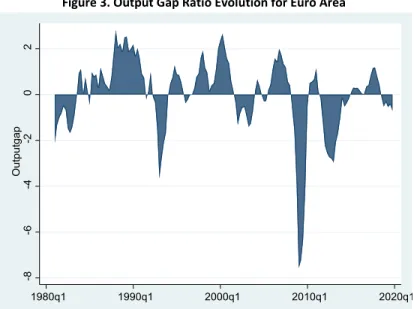
Figure 3 presents the output gap evolution. The Euro Area countries have faced several downturns in the past 30 years: Rapid exchange rate movements after entering the Euro Area in 1992-93, stock market bubble caused by excessive speculation in early 2000s, the Great Recession and Global Financial Crisis in 2008-09 and finally a period of low inflation which started in 2013 (Comunale and Mongeli, 2020).
Figure 3. Output Gap Ratio Evolution for Euro Area
3. Methodology
3.1 Bohn’s Contributions
A positive response of primary surpluses to changes in the debt-income ratio provides evidence for sustainability. As Bohn (1998) states, Trehan and Walsh (1988, 1991), Hakkio and Rush (1986), and Ahmed and Rogers (1995) applied standard Dickey-Fuller and Phillips-Perron unit root regressions and concluded the debt/GDP ratio as a nonstationary variable. Bohn (1998) argues that debt/GDP ratio is in fact stationary and the unit root regressions are misleading and shows that one can find direct evidence for corrective actions by examining the response of the primary surplus of the government budget to changes in the debt-income ratio. A positive
9
response shows that the government is taking actions (reducing noninterest outlays or raising revenue) that counteract the changes in debt.
Taking the equation for the primary surplus from Barro’s (1979) tax-smoothing model which illustrates the surplus-GNP ratio as follows:
𝑝𝑠𝑡 = 𝜌𝑑𝑡 + 𝛼0+ 𝛼𝐺 + 𝐺𝑉𝐴𝑅𝑡+ 𝛼𝑌+ 𝑌𝑉𝐴𝑅𝑡+ 𝜀𝑡, where
𝑝𝑠𝑡 =𝑆𝑡
𝑌𝑡 is the ratio of primary surplus to income, 𝑑𝑡 =
𝐷𝑡
𝑌𝑡 is the ratio of (start-of-period) debt to
aggregate income, GVAR is the level of temporary government spending and YVAR is the business cycle indicator.
Bohn (1998) demonstrates that this approach is more promising than a univariate time series analysis of the debt-income ratio because the debt-income ratio is in practice bounced around by various shocks (e.g., fluctuations in income growth, in interest rates, and in government spending) that make mean-reversion difficult to detect. Moreover, the unit root regressions are misspecified and inconsistent because they omit GVAR and YVAR. Therefore, there is strong evidence for mean reversion, provided that one accounts for fluctuations in GVAR and YVAR (Bohn, 1998).
Bohn (1998) further mentions that a stable debt/GDP ratio does not provide convincing evidence for sustainability. The reason is that, nonsustainable policies do not necessarily display an explosive debt-income ratio because of parameters such as real interest rate and the real growth rate in the government budget constraint equation.
The government budget equation can be written in ratio form as:
𝑑𝑡+1 = 𝑥𝑡+1 𝑑𝑡− 𝑠𝑡 , where 𝑥𝑡+1= 1 + 𝑅𝑡+1 𝑌𝑡
𝑌𝑡+1 ≈ 1 + 𝑟𝑡+1 − 𝑦𝑡+1 is the ratio of the gross return on government
debt to the gross growth rate of income and the variables 𝑟𝑡+1and 𝑦𝑡+1 denote the real interest rate and the real growth rate, respectively.
For example, if the government does not pay attention to the primary surplus and rolled over the existing debt with low interest rates, the debt/GDP ratio would decline in expectation. But this policy clearly violates the government budget constraint, and it is unsustainable if future growth falls below the interest rate with positive probability (Bohn, 1998). In his other studies, Bohn (1995, 2005) shows that average economic growth in the US economy has usually exceeded the average interest charge over the last 200 years. The U.S. Government succeed to keep its debt/GDP ratio from rising strength of the economic growth. In Europe, such long time series of interest and growth are not available, but Collignon (2012) shows that in the European Union,
10
growth rates often have exceeded after-tax interest rates over the last half century (Collignon, 2012).
Regardless of interest rates and growth rates comparison, a decrease in the primary deficit as a response to increase in the debt-income ratio does provide reliable information about sustainability. Hence, it is a strong test and valid in economies with arbitrary debt management policies, whether or not government bond rates are above or below the growth rate.
3.2 Empirical equations
Following the study and the methodology of Bohn (1998) which studies the US case, we investigate three related empirical models as Cassou, Shadmani and Vázquez (2017) considered in their study. The first and simplest model is a basic linear regression model, the second one is the threshold autoregressive model (TAR) and the third one is a Markov switching model. The last two models are nonlinear. The threshold model can be thought of as a two basic linear model nested in one regression that changes the coefficients according the chosen threshold. These nonlinear models allow us to investigate the asymmetries of fiscal policies within the business cycle. All of our models include only lagged variables as independent variables in order to understand the reaction of policy makers to the previous period at the time of execution.
The basic regression model is given by
𝑏𝑡 = 𝛼 + 𝛽1𝑏𝑡−1+ 𝛽2𝑑𝑡−1+ 𝛽3𝜔𝑡−1 + 𝜀𝑡
where 𝑏𝑡 is the ratio of the primary deficit (spending-net of interest expenses-revenues) to gross domestic product (GDP) at date t, 𝑑𝑡−1 is the ratio of government debt to GDP at date t−1, and
𝜔𝑡−1 is the output gap at date t −1, defined as the deviation of the observed annual output growth rate from its long-term value.
Bohn (1998) argues that an estimated value of β2<0 is sufficient for sustainability of fiscal policy in the sense that the government budget constraint is satisfied. Negative β2 values indicate that the decision makers try to balance the increase of debt/GDP ratio by reducing 𝑏𝑡 either by increasing revenues or cutting some expenditure. The sign of β3 depends on whether policy is pro-cyclical or counter-cyclical. Therefore an estimated positive value of β3 will indicate pro-cyclicality.
Nonlinear models, which allow the possibility of regime changes, enable us to understand the sustainability and the cyclicality of the fiscal policy and asymmetries in the states according to business cycles. Previously, some nonlinear models such as probit and logit have been used to predict US recessions. The threshold autoregressive (TAR) model is able to produce limit cycle, time irreversibility and asymmetry behavior of a time-series (Billio, 2009). Hence, part of our empirical focus will be on a popular asymmetry hypothesis in which the policy variable, 𝑏𝑡,
11
responds to the lagged covariates, differently, depending on whether the economy is strong or weak. Dummy variable It−1 shows whether the economy is in good times or bad times.
One difficulty in applying TAR models is the specification of the threshold variable, which plays a key role in the non-linear structure of the model. Akaike Information Criterion (AIC) and the Bayesian information criterion (BIC) procedure has been proposed and used by a large part of practitioners for the identification of a threshold parameter.
The threshold regression is given by
𝑏𝑡 = 𝛼𝐼𝑡−1+ 𝛽1𝐼𝑡−1𝑏𝑡−1+ 𝛽2𝐼𝑡−1𝑑𝑡−1+ 𝛽3𝐼𝑡−1𝜔𝑡−1+ 𝛼′(1 − 𝐼𝑡−1) + 𝛽1′(1 − 𝐼𝑡−1)𝑏𝑡−1+ 𝛽2′(1 − 𝐼𝑡−1)𝑑𝑡−1+ 𝛽3′(1 − 𝐼𝑡−1)𝜔𝑡−1+ 𝜀𝑡, where 𝐼𝑡−1 is given by It−1 = 0 for ωt−1 ≤ω T, 1 for ωt−1 >ωT, where ωT is the threshold value for the lagged output gap.
Markov switching (MS) models were first suggested by Hamilton (1989) in his seminal paper in order to assess GDP growth rates for two different regimes. These regimes depend on a unobservable variable that follows a Markov chain. The mean growth rate of GDP is subject to regime switching in Hamilton’s (1989) model. He uses an autoregressive model of order of four lags in order to analyze the business cycle relationship with growth rates. Kim and Nelson (1999) extended the Markov switching models to analyze business cycle effects by taking into account the comovement among economic variables through the cycle and the nonlinearity featuring its evolution. Hence the multivariate extension of the model generates results for economic variables within a business cycle.
The Markov switching model is given by
𝑏𝑡 = 𝛼(𝑠𝑡) + 𝛽1(𝑠𝑡)𝑏𝑡−1+ 𝛽2(𝑠𝑡)𝑑𝑡−1+ 𝛽3(𝑠𝑡)𝜔𝑡−1+ 𝛿(𝑠𝑡)𝜇𝑡,
where 𝑠𝑡 denotes the unobservable regime or state variable featuring the reaction of the fiscal authority to both variables entering into its information set (𝑏𝑡−1, 𝑑𝑡−1 and 𝜔𝑡−1) and the fiscal shocks (𝜇𝑡 ). For description purposes, this state variable has values of either 1 or 2. The first-order two-state Markov process with transition matrix of this state variable is given by
𝑃 = 𝑝11 1 − 𝑝22
12
where the row j, column i element of P is the transition probability 𝑝𝑖𝑗, which is the probability that state i will be followed by state j. The two regime Markov transition probabilities can be written as follows:
𝑝 𝑠𝑡 = 1 𝑠𝑡−1 = 1) = 𝑝11 , 𝑝 𝑠𝑡 = 2 𝑠𝑡−1 = 1) = 𝑝12 𝑝 𝑠𝑡 = 2 𝑠𝑡−1 = 2) = 𝑝22 , 𝑝 𝑠𝑡 = 1 𝑠𝑡−1 = 2) = 𝑝21,
where p11 + p12 = p21+ p22 = 1. The stochastic process for 𝑠𝑡is strictly stationary if both
𝑝11and 𝑝22 are less than unity and do not simultaneously take on the value of zero. When 𝑝11 =
1, once the process enters state 1, and then it would never return to state 2.
One type of MS model is the time-varying MS model (MS TVTP) which allows the transition probabilities to depend on an economic indicator such as output gap to understand the business cycle effects on the economy. As in Filardo (1994) the logistic functional form can be written as follows
𝑝11 𝜔𝑡−1 = exp 𝜃10+ 𝜃11𝜔𝑡−1 1 + exp 𝜃10+ 𝜃11𝜔𝑡−1 𝑝22 𝜔𝑡−1 = exp 𝜃20 + 𝜃21𝜔𝑡−1
1 + exp 𝜃20+ 𝜃21𝜔𝑡−1
𝜃11 and 𝜃21 coefficients are the impacts of the lagged output gap to the transition probabilities. When these coefficients (𝜃11 and 𝜃21) are equal to zero, the lagged output gap has no impact on the transition probabilities and the model becomes a Markov switching model with constant probabilities.3 Moreover, to infer some conclusions in terms of business cycles, 𝜃11 and 𝜃21
coefficients must be statistically significant and different from zero.
Threshold regression models and Markov switching models are similar but not the same. The main difference between the two models is that we can observe or decide the transition variable in threshold models, while in the MS models the states change according to an unobservable latent variable. Moreover, MS models allow for changes in the size of shocks across regimes and they also allow for the interaction of fiscal policy asymmetries with switches in shock volatility (Cassou et al., 2017).
3.3 Data
We use two sources of data for the Euro Area covering the period from 1980:1 to 2019:3. First, Paredes, Pedregal and Pérez (2014) created a quarterly database for the Euro Area until 2013:3.
3
Time-varying Markov switching model findings are not reported in this paper since the coefficients associated with output gap are not statistically significant.
13
We have completed this database data from 2013:q3 until 2019:q3 transforming available Eurostat data. The dataset covers the EA general government total revenue as a sum of EA general government total direct taxes, EA general government total social security contributions, EA general government total indirect taxes and the EA general government’s other revenues. As for the expenditure, EA general government total expenditure is the sum of Euro Area general government social payments (social transfers other than in kind, D62), EA general government interest payments, EA general government subsidies, EA general government consumption expenditure, EA general government investment and EA general government other expenditure. The database also includes Euro Area general government debt which consists of central, state and local governments and the social security funds controlled by these units.
Second, Fagan, Henry and Mestre (2001) created a quarterly database for the Euro Area, which is called Area Wide Model. The updated version of this database goes until 2017:q4. We have completed these series until 2019:q3 with data from the ECB’s Statistical Data Warehouse (SDW data). The dataset covers a wide range of quarterly Euro Area macroeconomic time series such as real GDP and the GDP deflator values.
Using the Parades at al. (2014) database, the primary deficit series was obtained by subtracting the total revenue (TOR) and interest payments (INP) from the total expenditure (TOE) and taking the ratio to nominal GDP. For the debt variable, we calculated the ratio of Euro Area general government debt (TRAMO) to nominal GDP.
For the output gap, we calculated the difference between the observed annual growth rate and the average annual growth rate using the Area Wide Model database. In particular, we computed the growth rate in percentage terms by multiplying 100 times the log difference between the current value of real GDP (YER) and the value four quarters earlier. Then, the average growth rate was subtracted from the annual growth rate series to obtain positive values when the current growth rate is above the average and negative values when the growth rate is below the average.
4. Results
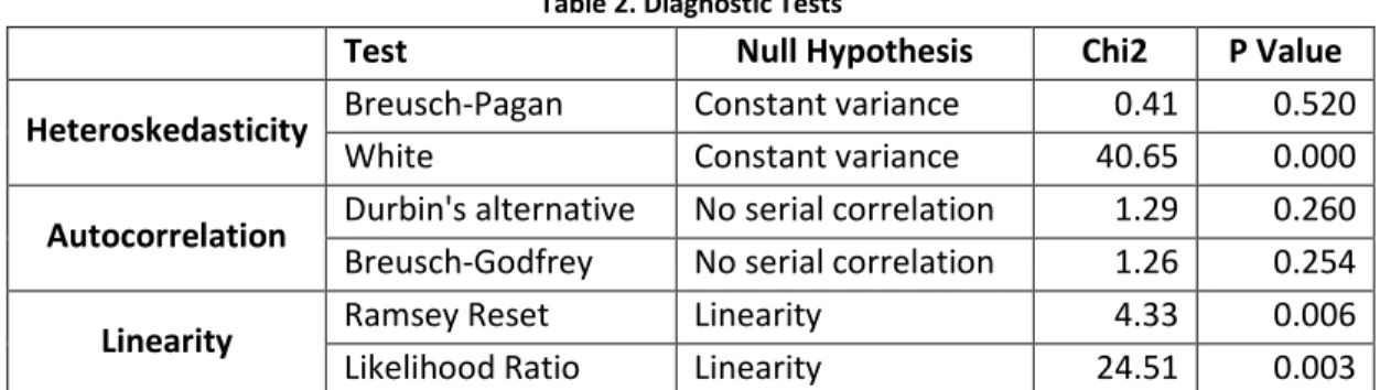
Table 2 summarizes the results of the heteroskedasticity and the autocorrelation tests as residuals diagnostic tests, the Ramsey reset test and the likelihood ratio test (LRT) as stability diagnostics tests. The Breusch-Pagan test indicates homoskedasticity while the White test infers the contrary, so we took into account non-constant variance in our models. For autocorrelation we apply Durbin's alternative and the Breusch-Godfrey tests, which both indicate no serial correlation. For linearity we applied the Ramsey regression equation specification error test (RESET) which is a general specification test for the linear regression model and the statistical test procedure suggested by Teräsvirta (1994). More specifically, these tests show whether non-linear combinations of the fitted values help to explain the response variable. As the p values are below the rejection area, we reject the null hypothesis which is linearity. Hence, non-linear models are appropriate for modeling fiscal policy.
14
Table 2. Diagnostic Tests
Test Null Hypothesis Chi2 P Value
Heteroskedasticity Breusch-Pagan Constant variance 0.41 0.520
White Constant variance 40.65 0.000
Autocorrelation Durbin's alternative No serial correlation 1.29 0.260
Breusch-Godfrey No serial correlation 1.26 0.254
Linearity Ramsey Reset Linearity 4.33 0.006
Likelihood Ratio Linearity 24.51 0.003
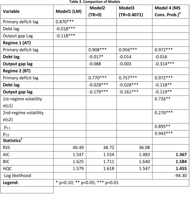
Table 3 shows the results for the different models. The first column describes these models according to their types. The first row shows the related variables and the statistics. Abbreviation of “AT” denotes above threshold and “BT” denotes below threshold. Markov switching models cannot be interpreted according to thresholds but to save space we put the results of MS model in terms of thresholds since the MS model have strong relations with business expansions and downturns. But, overall, threshold models and the MS models must have different interpretations.
In Table 3, regime 1 shows the results according to the MS model. These results have relation with good economic periods and regime 1 is determined according to the unobserved state variable s1. For the threshold models, regime 1 shows also good economic times but as above a certain value of the output gap, which shows strong economic growth. Similarly, regime 2 is determined by the unobserved state variable s2 which is related with economic downturns. For the threshold models this regime shows the linear portion of the model when the output gap is below a certain value which is associated with weak economic times.
To compare different types of models in terms of goodness of fit, we show three criteria which are commonly used in practice. First and the foremost is the Akaike information criterion (AIC) which is an estimator of out-of-sample prediction error and thereby relative quality of statistical models for a given set of data. Given a collection of models for the data, AIC estimates the quality of each model, relative to each of the other models. Thus, AIC provides a means for model selection. Second, Bayesian information criterion (BIC) which is a method for scoring and selecting a model, is appropriate for models fit under the maximum likelihood estimation framework. The Hannan-Quinn information criterion (HQC) as a third one is more consistent but less efficient than the others because of containing one more natural logarithm in the equation.
15
Table 3. Comparison of Models Variable Model1 (LM) Model2
(TR=0)
Model3 (TR=0.4071)
Model 4 (MS Cons. Prob.)4
Primary deficit lag 0.870***
Debt lag -0.018***
Output gap Lag -0.118***
Regime 1 (AT)
Primary deficit lag 0.908*** 0.956*** 0.972***
Debt lag -0.017* -0.014 -0.016
Output gap lag -0.088 -0.003 -0.314***
Regime 2 (BT)
Primary deficit lag 0.770*** 0.757*** 0.972***
Debt lag -0.028*** -0.028*** -0.118**
Output gap lag -0.179*** -0.161*** -0.119**
1st-regime volatility σ(s1) 0.726** 2nd-regime volatility σ(s2) 0.270*** p11 0.895** p22 0.943*** Statistics5 RSS 40.49 38.72 36.08 AIC 1.547 1.554 1.483 1.367 BIC 1.625 1.711 1.640 1.584 HQC 1.579 1.618 1.547 1.455 Log likelihood -94.30 Legend: * p<0.10; ** p<0.05; *** p<0.01
The basic regression model is presented in the second column which was run by using ordinary least squares (OLS) method. The abbreviation of LM indicates the linear model. This model does not separate the results according to the strong economic times or the weak economic times because it has no threshold. The results show sustainable and countercyclical fiscal policy in the Euro Area since the lagged debt and the lagged output gap coefficients are negative and highly
4 We have also studied the time varying Markov switching model which considers cyclical component of output to see business cycle effect. However, the two associated parameters with the output gap (θ11 and θ21) did not show statistically significance which means that time-varying MS model generally has same results with the constant probability MS model. Therefore, it is not reported in the table.
5
AIC, BIC and HQC values are reported in line with E-views software which calculates these criteria by dividing the values to the observation numbers.
16
significant. Moreover, the lagged primary deficit coefficient is highly significant and is close to one, which shows persistency in the primary deficit.
Since the Ramsey reset test and the likelihood ratio test indicate nonlinear models are appropriate for investigation, we allocate the rest of the columns to these models. Column 3 shows the results for threshold regression where the threshold value is chosen as zero for the lagged output gap and we show the short notation with TR=0 in parentheses. For below the threshold, coefficients are mostly similar with the previous linear model. However, there are important differences above the threshold: the estimated lagged primary deficit coefficient is highly significant and close to one. Below the threshold, our model shows a decrease in fiscal persistence as the value of the estimated coefficient becomes 0.77. Moreover, the lagged debt coefficient is negative and highly significant when the lagged output was below potential and significant when the economy was above potential, which indicates fiscal policy sustainability for both states. The coefficient is higher below threshold, which may show the decision makers are paying more attention for fiscal sustainability in the economic times of distress, probably to achieve the fiscal targets they needed. Moreover, the lagged output gap coefficients are negative for both states but only the below the threshold coefficient is significant, which shows counter-cyclical policy in weak economic times.
The fourth column of Table 3 presents the estimates of Model 3 for a TR model in which the threshold is endogenously chosen to obtain the best fit. The best fitting threshold for this model occurs at a lagged output gap value of 0.4071, which is higher than the zero threshold used in Model 2. The main difference of the best fitting model with the TR=0 model is that the lagged debt coefficient during good economic times becomes insignificant, which indicates nonsustainable fiscal policy for good economic times. The negative and significant coefficient of the lagged debt still shows strong sustainability in weak economic times. One possible interpretation is that the fiscal target concerns lose their importance during economic expansions because of confidence in economic strength that the fiscal targets would be achieved anyway. The lagged output gap coefficient during good economic times still remains insignificant as it is in the previous model. This is consistent with the results found in Balassone et al. (2010) for a sample of fourteen European Union countries which shows a strong counter-cyclical response when economic times of distress occur.
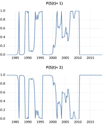
The fifth column of Table 3 shows the MS model with constant probability results which we name Model 4.6 Before discussing the findings in the MS model we should understand the Figure 4 that shows the relations of the regimes with the business cycles. Figure 4 shows the smoothed state probabilities for the MS model. As we can see, there are weak economic times for the Euro
6 According to the likelihood ratio test results at the appendix, restricted version of the model has e better fit. In this version we impose restriction on the lagged primary deficit to be same across the regimes. Hence, we report this model.
17
Area at the beginning of 80s, mid 90s, Great Recession period starting around 2010 and the sovereign debt crisis for Europe afterwards. These economic downturns are associated with state 2 whereas the expansionary periods are attributed to state 1. Therefore, we can say that states are somewhat related to the business cycles.
Figure 4 Transition Probabilities Markov Switching Model
The MS model has similar estimation results with the best fitting TR model in terms of fiscal policy sustainability. However, the coefficient of the lagged debt in weak economic times is higher in absolute value which shows stronger sustainable policy for MS model in economic times of distress. The lagged primary deficit coefficients of MS model are significant in both states and close to one which shows a tendency of persistency in the primary deficit. The response to the lagged output gap is symmetric, showing negative and significant coefficients in both states which shows the countercyclical fiscal policy. In short, the MS model exhibit sustainable policy in weak economic times and it shows counter cyclical fiscal policy in both regimes. The MS model differs with the best fitting threshold model in good economic times in terms of cyclicality of the fiscal policy. In terms of AIC, BIC and HQC, Markov switching model is the best fitting model among all the models. The results of MS model are consistent with the findings of Balassone et. al. (2010) for good economic times and with the findings of Golinelli and Momigliano (2006) in weak economic times. The MS model results are also in line
0.0 0.2 0.4 0.6 0.8 1.0 1985 1990 1995 2000 2005 2010 2015 P(S(t)= 1) P(S(t)= 1) 0.0 0.2 0.4 0.6 0.8 1.0 1985 1990 1995 2000 2005 2010 2015 P(S(t)= 2) P(S(t)= 2)
Markov Switching Smoothed Regime Probabilities Markov Switching Smoothed Regime Probabilities
18
with those found in Golinelli and Momigliano (2006), Hagen and Wyplosz (2008) and Arcabic (2018) in terms of cyclicality.
As explained in section 3.2, the TR regressions assume a constant volatility both above and below the threshold level while the regime volatilities change across the regimes in MS models. In state 1, volatility of the shock σ(s1), is roughly three times higher than the volatility of the shock in state 2, σ(s2). Therefore, regime 1 seems to identify not only good times but also more volatile times. Moreover, both volatilities are significant. Focusing on the transition probabilities of the MS model, the probability of staying in state 1 if one begins in state 1, p11, is high at 0.895, while the probability of staying in state 2 if one begins in state 2, p22, is higher at 0.943. These results show that there is high persistence for both states.
Overall, the LM exhibited sustainable and countercyclical behavior. The TR=0 model showed sustainable fiscal policy for both states and countercyclical fiscal policy only in weak economic times. The best fitting TR model showed that fiscal policy is neither sustainable nor cyclical in economic good times as the variables are not significant. The Markov switching model which is the best fitting model, indicate a sustainable and a countercyclical fiscal policy for weak economic times and unsustainable, countercyclical fiscal policy in the expansionary periods. The results of MS model are consistent with the findings of Balassone et. al. (2010) for good economic times and with the findings of Golinelli and Momigliano (2006) in weak economic times.
These findings can be interpreted as in the Euro Area decision makers pay attention to fiscal sustainability in the economic times of distress and they want to comply with the fiscal rules of EU as summarized in Section 2. For good economic times, policy makers tend to think that the economy would achieve the goals anyway as a result of increase in GDP which will decrease the debt/GDP ratio and deficit/GDP ratio levels automatically.
The MS model results are also in line with those found in Golinelli and Momigliano (2006), Hagen and Wyplosz (2008) and Arcabic (2018) in terms of cyclicality. This finding somewhat violates the normative prescription, pointed out in Cassou et. al. (2017) from Alesina et al. (2008), that the tax rates and discretionary government spending as a fraction of GDP should remain constant over the business cycle as advocated by most economists.
19
5. Conclusions
In mid-September 2008 the Great Recession and the sovereign debt crisis hit the Euro Area severely. Some countries have faced default risk while others have exceeded their targets. As a result, the EU started to pay more attention to sustainable fiscal policy as the Union has introduced new regulations and approaches to maintain the policy in a balanced way.
This paper analyzes fiscal policy sustainability and the cyclicality in 19 Euro Area countries using data on government debt, primary deficit and the output gap. We use the primary deficit/GDP ratio as the decision variable in a policy response function for the sustainability analysis where it is a function of its own lag and the lagged values of government debt/GDP ratio and the output gap. In this framework, a negative coefficient associated with the debt/GDP ratio suggests that policymakers react by reducing the primary deficit/GDP ratio against the debt/GDP ratio increases and thus it is a sign for sustainable fiscal policy.
Our estimation results show that primary deficit/GDP ratio responds negatively to an increase in government debt in weak economic times, which we interpret as sustainable fiscal policy in the economic times of distress. However, both best fitting threshold model and the Markov switching model do not support this idea during economic expansions. Hence, we interpret the robust sustainable results during times of distress as evidence that policy makers are concerned about the fiscal rules and targets in weak economic times. Regarding the cyclicality of fiscal policy, we find symmetric and countercyclical behavior in the Markov switching model. Both threshold models again indicate that the policy is countercyclical only in weak economic times.
In this respect, we can conclude that the fiscal goals for public debt and deficit set by the Stability and Growth Pact are essential tools to ensure fiscal sustainability and together with the dynamic corrective measures, fiscal rules would be helpful for fiscal sustainability. Certainly, the rapid increases in the debt/GDP ratios across Euro Area countries due to the current COVID-10 crisis will stress again the importance of effective fiscal corrective measures to achieve fiscal sustainability in the near future.
20
6. References
Annett, A. (2006). “Enforcement and the stability and growth pact: how fiscal policy did and did not change under Europe’s fiscal framework”, IMF Working Paper, No. 116.
Balassone, F., Francese, M. and Zotteri, S. (2010). “Cyclical asymmetry in fiscal variables in the EU”. Empirica, 37(4), pp. 381-402.
Balassone F., Cunha J., Langenus G., Manzke B., Pavot J., Prammer D. Tommasino P. (2009). “Fiscal Sustainability And Policy Implications For The Euro Area”, European Central Bank. Billio M., Ferrara L., Guegan d., Mazzi G.L. (2009). “Evaluation of nonlinear time-series models for real-time business cycle analysis of the Euro Area”, HAL-00423890.
Bohn, H. (1998). “The behavior of US public debt and deficits”, The Quarterly Journal of Economics, 113(3), pp. 949-963.
Bohn, H. (2007). “Are stationarity and cointegration restrictions really necessary for the intertemporal budget constraint?”, Journal of Monetary Economics, 54(7), pp. 1837-1847.
Burnside C. and Meshcheryakova Y. (2004). “Mexico: a case study of procyclical fiscal policy”, November, International Monetary Fund.
Cassou, S. P., Shadmani, H. and Vázquez, J. (2017). “Fiscal policy asymmetries and the sustainability of US government debt revisited”, Empirical Economics, 53(3), pp. 1193-1215.
Cecchetti S.G., Mohanty M.S. and Zampolli F. (2011). “The real effects of debt”, BIS Working Paper 352.
Collignon, S. (2012). “Fiscal policy rules and the sustainability of public debt in Europe”, International Economic Review, 53(2), pp. 539-567.
Comunale M. and Mongelli F. P. (2020). “Tracking long-run growth in the euro area with an atheoretical tool: The role of real, financial, monetary, and institutional factors”, CAMA working paper, https://voxeu.org/article/tracking-long-run-growth-euro-area-atheoretical-tool
Debrun, X. and Kumar M.S. (2006), “The discipline-enhancing role of fiscal institutions: theory and empirical evidence”, European Commission on the role of national fiscal rules and institutions in shaping budgetary outcomes, Bruxelles, 24 November.
Egert B. (2010), “Fiscal policy reaction to the cycle in the OEC: pro- or counter-cyclical?”, OECD Economics Department Working Papers No. 763.
21
Eurofi (2019), “Policy Note Regulatory Update”, Eurofi Secretariat, https://www.eurofi.net/wp-content/uploads/2019/11/are-sovereign-debts-sustainable-in-the-eu_bucharest_april2019.pdf
EU Commission (2017), “European Semester Thematic Factsheet Sustainability Of Public Finances”, https://ec.europa.eu/info/sites/info/files/european-semester_thematic-factsheet_public-finance-sustainability_en_0.pdf
Fagan,G., Henry J. and Mestre R. (2001) “An Area-wide Model (AWM) for the Euro Area” ECB working paper No. 42.
Fatas A., Mihov I. (2003), “The case for restricting fiscal policy discretion”, The Quarterly Journal of Economics, vol. 118, issue 4, 1419-1447.
Golinelli R, Momigliano S. (2008). “The cyclical response of fiscal policies in the Euro Area. why results of empirical research differ so strongly?”, Banca d’Italia Temi di Discussione 654.
Golinelli, R. and Momigliano S. (2006). “Real-time determinants of the fiscal policies in the Euro Area”, Journal of Policy Modeling, Vol. 28, pp. 943-64.
Killinger N. and Nerlich C. (2019), “Fiscal rules in the euro area and lessons from other monetary unions”, ECB Economic Bulletin, Issue 3/2019.
Lojsch D.H., Vives M.R., and Slavík M. (2011), “The size and composition of government debt in the Euro Area, ECB Occasional Paper Series”, No 132 / October 2011.
OECD (2010), “Restoring fiscal sustainability: lessons for the public sector”, Public Governance Committee Working Party of Senior Budget Officials.
OECD (2013), "Fiscal sustainability", in Government at a Glance 2013, OECD Publishing, Paris,
https://doi.org/10.1787/gov_glance-2013-11-en
OECD (2017), “Government at a Glance”, OECD Publishing, Paris,
https://doi.org/10.1787/gov_glance-2017-8-en
Paredes J, Pedregal, D. J.,Perez, J. (2014), “Fiscal policy analysis in the Euro Area: expanding the toolkit”, Journal of Policy Modeling, Volume 36, Issue 5, September–October, Pages 800-823, ISSN 0161-8938.
Reinhart C.M. and K.S. Rogoff, (2010). “Growth in a time of debt”, American Economic Review, 100 (2): 573–78.
Peltier H. G. (2014), "The job opportunity cost of war," Watson Institute.
Von Hagen J., Wyplosz C. (2008), “EMU’s decentralized system of fiscal policy, Europen Commission”, Economic and Financial Affairs, Economic Papers 306.
22
7. Appendix
7.1 Key Indicators for The Euro Area
23
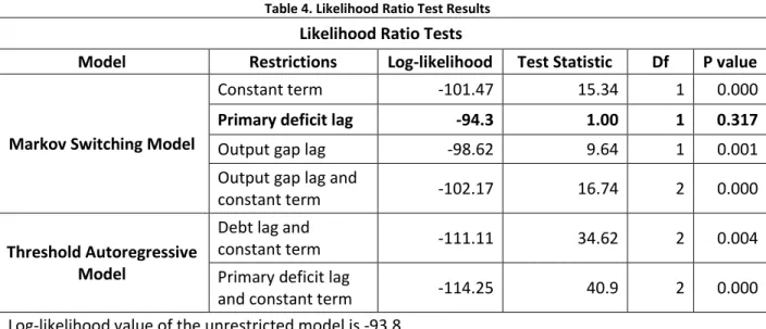
7.2 Likelihood Ratio Test Results
Table 4. Likelihood Ratio Test Results Likelihood Ratio Tests
Model Restrictions Log-likelihood Test Statistic Df P value
Markov Switching Model
Constant term -101.47 15.34 1 0.000
Primary deficit lag -94.3 1.00 1 0.317
Output gap lag -98.62 9.64 1 0.001
Output gap lag and
constant term -102.17 16.74 2 0.000
Threshold Autoregressive Model
Debt lag and
constant term -111.11 34.62 2 0.004
Primary deficit lag
and constant term -114.25 40.9 2 0.000
Log-likelihood value of the unrestricted model is -93.8
Likelihood ratio tests compare two models in order to decide whether to reject a restriction on the parameter. So in order to check which model fits significantly better, we imposed some restrictions on the model variables. Then we computed the test statistic using the formula LR=−2ln(L(m1)/L(m2))=2(loglik(m2)−loglik(m1)) Where m1 is the more restrictive model, and m2 is the less restrictive model. Lower associated p-value, indicates that the model with less restricted or unrestricted model fits significantly better than the model with restricted.
As we can see from the Table 4, we have checked various models whether they fit better or not and we conclude that restricted model with restriction to lagged primary deficit fits better than the unrestricted model.
7.3 Simple Correlations of the Variables
Table 5. Correlations of the Variables
Primary deficit Debt Output gap Primary deficit lag debt lag Output gap lag Primary deficit 1 Debt -0.65 1 Output gap 0.02 -0.18 1
Primary deficit lag 0.97 -0.64 -0.11 1
Debt lag -0.67 1.00 -0.15 -0.66 1