A University of Sussex MPhil thesis
Available online via Sussex Research Online:
http://sro.sussex.ac.uk/
This thesis is protected by copyright which belongs to the author.
This thesis cannot be reproduced or quoted extensively from without first
obtaining permission in writing from the Author
The content must not be changed in any way or sold commercially in any
format or medium without the formal permission of the Author
When referring to this work, full bibliographic details including the aut
hor, title, awarding institution and date of the thesis must be given
perspective
Linghua Zhang
Thesis submitted for the
Degree of Master of Philosophy
University of Sussex
June 2016
University of Sussex Linghua Zhang
Degree of Master of Philosophy
Option volatility study from a data analysis perspective Summary
In this research, we will investigate both financial option pricing models and link the theory to real market performance studies. By combining traditional option pricing theory and real market data analysis, we propose that, in the real world, some behaviour of the financial option price is strongly associated with the local maximum or minimum of asset price.
Firstly, we analyse some mathematical formulas and theorems to understand how to simulate the random process of asset price movement. Based on these foundations we discuss Black-Scholes option pricing model, stochastic volatility models and numerical methods to price options.
Secondly, we utilise Monte-Carlo simulation to learn about the mechanisms of European option pricing with different models. Subsequently, regression analysis is presented in preparation for studying real market data analysis.
Thirdly, we use nine years of real market data to reveal the relationship among variables involved in pricing European options. It will be concluded that the implied Black
-Scholes risk calculated using real world call options and put options correlates with asset prices in opposing ways. For call options: with dominant probability, the instantaneous implied option risk and the asset price have a negative correlation;; whereas with dominant probability, one-day earlier implied option risk and the asset price have a positive correlation. Put options are the exact opposite.
Finally, we conclude that when the real market option prices are undervalued, they have the ability to catch local extreme values of asset prices statistically.
Acknowledgements
My greatest thanks must go to my supervisor, Dr. Qi Tang. I would like to thank his supporting, caring, understanding, sharing and guiding during my study at the University of Sussex. He was very kind and patient when I have any questions. His positive attitude towards life and humorous lectures also impressed me a lot. Without his help, this thesis could not have been completed.
Furthermore I would like to express my thanks to my parents, especially my mother. She always supported me whatever I want to do, wherever I want to go. I am so grateful to be her daughter.
In addition, I would like to thank all the people who have worked with me. They helped me to understand and realize more points that I have never thought about. I think my learning ability increased a lot thanks to their help.
Additionally, I wish to express my thanks to the examiners Dr. Bertram During and Dr. Katerina Tsakiri. Thanks their suggestions for my thesis.
Finally, I wish to sincerely thank all my friends. They always cheer me up on my bad days and make me feel positive.
Contents
1 Introduction ...
1
1.1 Introduction to financial derivatives ... 1
1.2 History of option trading ... 4
1.3 The use of financial options... 5
1.4 Introduction to Black-Scholes implied volatility on European options ... 6
2 Background and foundation ...
8
2.1 Mathematical background... 8
2.2 Financial background ... 13
2.2.1 No-arbitrage argument ... 13
2.2.2 Price of options ... 14
2.2.3 Put-call parity ... 16
2.2.4 Bounds on prices of European options ... 17
3 Models...
19
3.1 Black-Scholes option pricing model ... 19
3.1.1 Black-Scholes model ... 19
3.1.2 Formulas for the European call and put options prices ... 21
3.2 Stochastic volatility models ... 23
3.2.1 Hull-White stochastic model ... 23
3.2.2 Heston model ... 23
3.3 Numerical methods ... 24
3.3.1 Binomial methods ... 24
3.3.2 Pricing European option with binomial methods ... 28
4 Simulation and regression ...
32
4.1 Monte-Carlo simulation for pricing European options ... 32
4.1.1 Monte-Carlo simulation using standard Brownian model ... 32
4.1.2 Monte Carlo simulation using Hull-White model ... 34
4.1.3 Monte-Carlo simulation using Heston model ... 37
4.2 Regression ... 40
4.2.1 Linear regression ... 40
4.2.2 Measure goodness of fit ... 42
5 Real life data analysis ...
45
5.1 Introduction to data used ... 45
5.2 Correlation between implied volatility and asset returns ... 49
5.3 Variance capture ... 52
5.4 Negative risk study ... 57
5.5 Results and discussions ... 59
1 Introduction
In this dissertation, we study real world financial option prices and their corresponding Black-Scholes implied volatilities. It is apparent that these real world implied volatilities, if plotted along the strike price and time to maturity as a surface, the structure becomes coarse and do not follow the theory of standard volatility surface which is assumed to be smooth according to standard text books. It is therefore interesting for us to investigate how these implied volatilities interact with the underlying asset prices.
In the subsections 1.1-1.4 of the introduction, we discuss the standard definition and related properties of financial options. In Section 2, we discuss financial backgrounds and related mathematical tools required for our study. In Section 3, we discuss the Black-Scholes option pricing model and some stochastic volatility models presented in various studies. We also examine the corresponding numerical methods for pricing options. In Section 4, we demonstrate Monte-Carlo simulation of different models and regression analysis. In Section 5, we discuss some properties of the implied volatility of real world option data, establishing links between implied volatility and asset price movements.
1.1
Introduction to financial derivatives
Financial market instruments (Etheridge, 2004) can be divided into two distinct types. The first type consists of those representing a fraction of a real underlying asset: shares (fraction of a company), bonds (a nominal sum of money), commodity contracts (a certain quantity of a particular metal, agricultural product etc.), and foreign currencies. The second type consists of their derivatives, mostly comprising promises to deliver some kind of value in the future dependent on the behaviour of the corresponding underlying assets.
A statement in the cover story of The Economist magazine on the 14 May 1994 expertly describes the concept of financial derivatives: financial derivatives are contracts, which give one party a claim on an underlying asset or the cash value of the underlying asset at
some point in the future, and bind a counter-party to meet the corresponding liability. The contract might be described by a nominal amount of currency, a number of units of a security, a defined quantity of a physical commodity, a stream of cash payments, or the value of a market index. It might bind both parties equally, or offer one party an option to exercise it or not. It might provide for assets or obligations to be swapped in a predefined formula. It might also be a bespoke derivative combining several elements. Derivatives can be traded either on the stock exchanges or simply over the counter between two or several counter parties;; their current market prices usually depend partly on the movement of the prices of the underlying assets after the contracts are created. From a mathematical perspective, the price of a financial derivative is a function of the underlying asset price as well as a possible number of other variables, such as interest rates, time to maturity, volatility of markets or other factors.
Financial derivatives can be classified into four categories: forwards, futures, options and swaps. In this paper, options will be examined.
Definition 1.1.1: Financial options
A financial option is a contract written on an underlying asset. This contract gives the buyer the right but not the obligation to buy or sell the underlying asset on a specified price, K, before/on specified time, T, and gives the seller the obligation to fulfill the corresponding rights of the buyer.
Option buyers need to pay option premiums to the sellers (writers) to compensate the option sellers’ duty to fulfill the obligation when the underlying price moves in the favour of the buyers, while allowing the buyers to abandon the contract should the underlying price move against them.
If an option is written to buy the underlying asset, it is called a call option. If an option is written to sell the underlying asset, it is called a put option.
Type Trade side Expectation for underlying asset
Premium Duty Maximum
profit
Maximum loss
Call
Buyer Increase Pay Right, no
obligation Infinite Premium Seller Decrease Collect Obligation,
no right Premium Infinite
Put
Buyer Decrease Pay Right, no
obligation Infinite Premium Seller Increase Collect Obligation,
no right Premium Infinite Table 1.1.1 Differences between call and put options
The difference between a European option and an American option is that a European option written at 𝑡 = 0 can only be exercised at the maturity time 𝑡 = 𝑇. An American option written at 𝑡 = 0 can be exercised at any time between 𝑡 = 0 and 𝑡 = 𝑇.
Hence, a European call (put) option gives the buyer the right, but not the obligation to purchase (sell) one unit of the underlying asset at a specified time, T, for a specified price, K.
In the real financial world, only European options have comprehensive data available because they have well defined OE (option expiring) days. Thus, we focus on European options in this dissertation.
Definition 1.1.2: The exercise date/the maturity
The exercise date or the maturity is the time T at which the option contract expires.
Definition 1.1.3: The strike price
A call option is defined to be in the money, if the spot price is greater than the exercise price K, it is at the money if the spot price is equal to K, and it is out of the money if the spot price is less than K.
For a put option, it is in the money if the stock price is lower than the exercised price K, it is at the money if the spot price is equal to K, and it is out of the money if the spot price is greater than K.
Call options Put options In-the-money Strike price<Asset price Strike price>Asset price At-the-money Strike price=Asset price Strike price=Asset price Out-of-the-money Strike price>Asset price Strike price<Asset price
Table 1.1.2 Classification of options in(out)-of-the-money
1.2
History of option trading
Thompson (2007) stated that the Dutch parliament considered a decree (originally sponsored by the Dutch tulip investors who had lost money because of a German setback during the Thirty Years' War) that changed the way tulip contracts functioned: on 24 February 1637, the self-regulating guild of Dutch florists, in a decision that was later ratified by the Dutch Parliament, announced that all futures contracts written after 30 November 1636 and before the re-opening of the cash market in the early Spring, were to be interpreted as option contracts. They did this by simply relieving the futures buyers of the obligation to buy the future tulips, forcing them merely to compensate the sellers with a small fixed percentage of the contract price.
Before this parliamentary decree, the purchaser of a tulip contract – known in modern finance as a futures contract – was legally obliged to buy the bulbs. The decree changed the nature of these contracts, so that if the current market price fell, the purchaser could
opt to pay a penalty and forgo the receipt of the bulbs, rather than pay the full contracted price. This change in law meant that, in modern terminology, the futures contracts had been transformed into options contracts.
Alexander (2008, p. 137) highlights that the first exchange listed options in the world were on the Marche a Prime in France. At that time, about 10 per cent of trading on shares was carried out in this market, where shares were sold accompanied with a three
-month at-the-money put option. Due to the existence of this market, in 1900 Louis Bachelier devised a formula to evaluate options premiums based on arithmetic Brownian motion. Subsequently, during the 1930s, gold options were independently traded in Germany. However as they are difficult to value, these options were not popular during the period.
Decades later in 1973, the Chicago Board of Options Exchange (CBOE) was founded and became the first modern, comprehensive marketplace for trading listed options. In the same year, Black and Scholes published a price formula (Black and Scholes, 1973;; Merton, 1973, p. 639) revealing how to value a financial option based on geometric Brownian motion. It was the first systematical tool that received the public’s approval and is still widely used as a referencing valuation tool today.
In recent years, financial options are traded either over the counter (OTC) or on official stock exchanges.
1.3
The use of financial options
i. Speculation
If an investor believes that a particular share price is going to rise within a period T to a level much higher than K, he/she can buy a call option with exercise price K and expiry date T with the intention to make a profit. For example we suppose K is 25, the share price today is 25, an option on 𝐾 = 25 and 𝑇 = 1 year costs 1. If the share price at the expiry date goes up to 27, then the investor who buys this option for and holds it until 𝑡 = 𝑇 will make a 100 per cent profit (profit = 2, cost = 1, by ignoring minor factors such as trading costs and interest costs).
ii. Hedging
Suppose that an investor already owns a particular share as a long-term investment and maybe in a situation which is inconvenient to sell (e.g. the holding is large). In
S0
ST
this case, the investor may wish to insure against a temporary fall in the share price. Accordingly they can buy a put option to protect financial losses caused by the asset price decreasing. If the underlying asset price decreases, the investor can make a profit from the put option to compensate the loss from holding the underlying asset.
1.4
Introduction to Black-Scholes implied volatility on
European options
Option volatility is a measure of the rate and magnitude of the change of underlying prices. Black-Scholes implied volatility is calculated by inverting the Black-Scholes formula (Black and Scholes, 1973) when option price and all other factors are provided. According to this perspective, suppose that the fixed risk-free interest rate is 𝑟, strike price is fixed at K, and maturity is fixed at T, then the market price 𝑓(𝑆, 𝜎, 𝑡) of a standard European call or put option can be calculated from the market price S of the underlying asset using the following formula:
𝑓(𝑆, 𝜎, 𝑡) = 𝜔𝑁(𝜔𝑑 )𝑆 − 𝜔𝑁(𝜔𝑑 )𝐾exp(−𝑟(𝑇 − 𝑡)) , (1.4.1) with ( ) 2 ln 1 2 1 r T t K S t T d and 𝑑 = 𝑑 − 𝜎√𝑇 − 𝑡, where
for a call option and 𝜔 = −1 for a put option, and 𝑁(∙) is the cumulative normal distribution density function. The unknown value of 𝜎 that satisfies Equation (1.4.1) is the implied volatility. It is straightforward to find this value using MATLAB.
The Black-Scholes model (Black and Scholes, 1973) assumes that the variance rate of the return on the stock is constant for all possible values of strike price and maturity dates. Meanwhile, implied volatility using real world option prices always show different values for different strikes and maturity dates (Chen and Xu, 2013). Rubinstein (1994, p. 776) and Bakshi et al. (1997, p. 2022) used real world Standard & Pool’s 500 (S&P) option data to calculate implied volatility and confirmed that implied volatility is not constant. They concluded that the implied volatility of S&P 500 options show a ‘smile’ pattern across the strike price. Thereafter, some researchers explored further this
=
1
phenomenon (Bates 1996, p. 169, Dumas, Fleming & Whaley 1998, p. 2061) and found that, after 1987, the implied volatility of S&P 500 options was monotone with the moneyness or the strike price, and therefore it exhibited a so-called volatility ‘sneer’ instead of a volatility ‘smile’.
Considering the aforementioned observations, an increasing number of researchers began to investigate implied volatility for financial options determined by option prices. In recent years, researchers have introduced some alternative volatility models which have demonstrated that implied volatility had some mathematical forms other than a constant. The models include, for example, the jump diffusion model devised by Merton (1976, p. 132), the stochastic volatility models (Hull and White 1987, p. 288;; Chesney and Scott 1989, p. 268;; Stein and Stein 1991, p. 744;; Heston 1993, p. 331), and the deterministic local volatility model (Dupire, 1994, p. 128;; Derman and Kani 1994;; Rubinstein 1994, p. 785).
2 Background and foundation
In this chapter, concepts concerning financial options will be introduced on two fronts
- the mathematical theory front and the financial theory front. As will be explained, the value of financial options is a function of the underlying price, volatility of the underlying assets, exercise price, interest rate and time to maturity. In Section 2.1, the necessary mathematical tools that are needed to derive the formula for evaluating values of financial options is introduced. In Section 2.2, financial terminologies and concepts for defining option values are discussed.
2.1 Mathematical background
In this section we introduce some mathematical definitions. Firstly, random walk and Brownian motion or Wiener process, which are used to simulate the movement of the underlying asset price, will be presented. By applying Ito’s formula (Ito, 1944) to the random walk model, we deduce the mathematical formula of geometric Brownian motion, which plays a pivotal role in analysing and simulating stock prices.
Definition 2.1.1: Random Walk
A random walk is a mathematical description of a path that consists of a succession of random steps. Feller (1971, p. 24) described it as follows:
Let 𝑋(1), 𝑋(2), … , 𝑋(𝑁) be independent random variables with values -1 or 1 in equal probability. A random walk is the sequence of random variables
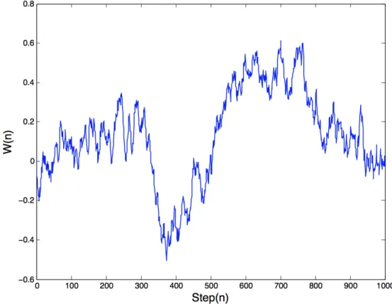
𝑆(0) = 0, 𝑆(𝑛) = ∑ 𝑋(𝑖) , 𝑛 = 1,2, … , 𝑁. (2.1.1) We simulate a random walk for 100 steps in the following graph so that we can understand intuitively what it means.
Figure 2.1.1 Random Walk
The steps range from 0 to 100 means n varies from 0 to 100.
Now we introduce the mathematical definitions required to describe random walk in a rigorous setting:
First, we specify a probability triple (Ω, ℱ, ℙ), where Ω is a set, called the sample space;;
ℱ is a collection of subsets of Ω, called events;; and ℙ specifies the probability of each event 𝐴 ∈ ℱ. The events collection ℱ is a 𝜎 −field, that is, Ω ∈ ℱ and ℱ is closed under the operations of countable union and taking complements. The probability ℙ must satisfy the usual axioms of probability (Etheridge, 2002):
· 0 ≤ ℙ[𝐴] ≤ 1 for all 𝐴 ∈ ℱ,
· ℙ[Ω] = 1,
· ℙ[𝐴⋃𝐵] = ℙ[𝐴] + ℙ[𝐵] for any disjoint A, B ∈ ℱ,
· if 𝐴 ∈ ℱ for all 𝑛 ∈ ℕ and 𝐴 ⊆ 𝐴 ⊆ ⋯ then ℙ[𝐴 ] ⟶ ℙ[∪ 𝐴 ] as 𝑛 → ∞.
A collection of {ℱ } where ℱ ⊆ ℱ ⊆ ⋯ ⊆ ℱ is called a filtration and if a filtration is given, the quadruple (Ω, ℱ, {ℱ } , ℙ) is called a filtered probability space (Etheridge, 2002).
Definition 2.1.2: Random variables (Etheridge, 2002)
A real-valued random variable 𝑋 is a real-valued function on 𝛺 that is ℱ −measurable. In the case of a discrete random variable this simply means that for any 𝑥 ∈ 𝑅,
{𝜔 ∈ 𝛺: 𝑋(𝜔) = 𝑥} ∈ ℱ,
so that ℙ assigns a probability to the event {𝑋 = 𝑥}. For a general real-valued random variable, we require that for any 𝑥 ∈ 𝑅
{𝜔 ∈ 𝛺: 𝑋(𝜔) ≤ 𝑥} ∈ ℱ,
so that we can define the distribution function, 𝐹(𝑥) = ℙ[𝑋 ≤ 𝑥].
Definition 2.1.3: Stochastic processes
A real-valued stochastic process is just a sequence of real valued functions, {𝑋 } , on
𝛺. We say that it is adapted to the filtration {ℱ } if 𝑋 is ℱ −measurable for each (Etheridge, 2002).
Definition 2.1.4: Brownian Motion/ Wiener process
A real-valued stochastic process {𝑊(𝑡)} is a ℙ −Brownian motion (or ℙ −Wiener process) if for some real constant 𝜎, under ℙ (Etheridge, 2002),
· for each 𝑠 ≥ 0 and 𝑡 > 0 the random variable 𝑊(𝑡 + 𝑠) − 𝑊(𝑠) follows the
normal distribution with mean zero and variance 𝜎 𝑡,
· for each 𝑛 ≥ 1 and any time sequence 0 ≤ 𝑡 ≤ 𝑡 ≤ ⋯ ≤ 𝑡 , the random variables {𝑊(𝑡 ) − 𝑊(𝑡 )} are independent,
· 𝑊(0) = 0,
· 𝑊(𝑡) is continuous in 𝑡 ≥ 0, which means lim
→ 𝐸
| ( ) ( )|
| ( ) ( )| = 0.
We simulate a Brownian motion in Figure 2.1.2 for 1000 steps so that we can understand intuitively what it means.
Figure 2.1.2 Brownian motion/Wiener process
Definition 2.1.5: Stochastic differential equation
A typical stochastic differential equation is of the form (Bichteler, 2002)
𝑑𝑋(𝑡) = 𝜇(𝑋(𝑡), 𝑡)𝑑𝑡 + 𝜎(𝑋(𝑡), 𝑡)𝑑𝑊(𝑡), (2.1.2) where the function 𝜇 is referred to as the drift coefficient;; the function 𝜎 is called the diffusion coefficient;; 𝑊 denotes a Brownian motion/Winner process.
The integral form of the differential equation (2.1.2) can be written as
𝑋(𝑡) − 𝑋(0) = ∫ 𝜇(X(s), s)𝑑𝑠 + ∫ 𝜎(X(s), s)𝑑𝑊(𝑠).
Definition 2.1.6: 𝐈𝐭𝐨’s Formula
If is a stochastic process, satisfying dXt tdt tdWt, and f is a deterministic
twice continuously differentiable function, then 𝑌 ≔ 𝑓 (𝑋 , 𝑡) is also a stochastic process and the differential equation of 𝑌 is given by
𝑑𝑌 = 𝜇 + + 𝜎 𝑑𝑡 + 𝜎 𝑑𝑊. (2.1.3)
Definition 2.1.7: Geometric Brownian motion
Geometric Brownian motion is a continuous-time stochastic process in which the logarithm of the random variable follows a Brownian motion with drift.
A stochastic process 𝑆(𝑡) is said to follow a Geometric Brownian motion if it satisfies the following stochastic differential equation
𝑑𝑆(𝑡) = 𝜇𝑆(𝑡)𝑑𝑡 + 𝜎𝑆(𝑡)𝑑𝑊(𝑡), for 𝑡 > 0, (2.1.4) with a constant drift 𝜇, and a constant volatility 𝜎, where 𝑊 is a Wiener process (also called Brownian motion).
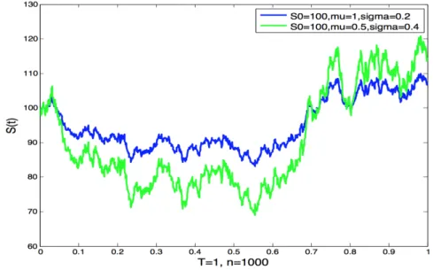
For an arbitrary initial value 𝑆 the above stochastic differential equation has the analytic solution (Hull, 2009, p. 271)
𝑆(𝑡) = 𝑆 exp 𝜇 − 𝑡 + 𝜎𝑊(𝑡) . (2.1.5) We simulate two geometric Brownian motions with different drifts and volatilities so that we can understand intuitively what it means. The simulation is displayed as below:
2.2 Financial background
In this section, a brief introduction to some key financial terms is presented in order to make them more meaningful, including no-arbitrage argument for the derivation of option price formula, option contracts, some relationships between call options and put options and the bounds on prices of options.
2.2.1 No-arbitrage argument
Schachermayer(2002) argues that, ‘the principle of no-arbitrage formalises a very convincing economic argument: in a financial market it should not be possible to make a profit with zero net investment or without bearing any risk’.
For the purposes of this study, no-arbitrage is divided into weak no-arbitrage and strong no-arbitrage. They are introduced with the following definitions and examples.
Definition 2.2.1: Weak no arbitrage
In an investment scheme, let 𝑝 be the price to pay at time 𝑡 = 0, 𝐶 be the payoff at time
𝑘 = 1,2, … 𝑇. Weak no arbitrage assumption means that when 𝐶 ≥ 0, for all 𝑘 ≥ 1, we must have 𝑝 ≥ 0.
Justification: Suppose 𝑝 < 0.
Since 𝐶 ≥ 0 for all 𝑘 ≥ 1, the buyer receives – 𝑝 > 0 at time 𝑡 = 0, and then does not lose money thereafter. This brings potential profit for no investment (receiving money at the beginning). The seller can increase 𝑝 as long as 𝑝 < 0, and still have buyers available because the riskless profit opportunity still exists.
Hence 𝑝 could not be less then zero.
Definition 2.2.2: Strong no arbitrage
In an investment scheme, let 𝑝 be the price to pay at time 𝑡 = 0, 𝐶 be the payoff at time
𝑘 = 1,2, … 𝑇. Strong no arbitrage assumption means that when 𝐶 ≥ 0 for all 𝑘 ≥ 1
Justification: Suppose p ≤ 0.
Since 𝐶 ≥ 0 for all 𝑘 ≥ 1, and for some 𝑙 ≥ 1, 𝐶 > 0, which means that the buyer makes profit at some time when 𝐶 > 0. The buyer receives – 𝑝 ≥ 0 at time 𝑡 = 0, and then makes profits thereafter. This brings potential profit for no investment (receiving money at some time 𝑡 = 𝑙). The seller can increase 𝑝 as long as 𝑝 ≤ 0, and still have buyers available because the riskless profit opportunity still exists.
Hence 𝑝 must be greater than zero.
Type A and Type B arbitrage
Definition 2.2.3: Type A arbitrage is a security or portfolio that produces immediate positive reward at 𝑡 = 0 and has non-negative value at 𝑡 = 1.
Example 2.2.1: Suppose 𝑉 is price of a security at time t. The security with initial cost
𝑉 < 0 and at time 𝑡 = 1 value 𝑉 ≥ 0 is an example of type A arbitrage.
Definition 2.2.4: Type B arbitrage is a security or portfolio that has a non-positive initial cost which has positive probability of yielding a positive payoff at 𝑡 = 1 and zero probability of producing a negative payoff at 𝑡 = 1.
Example 2.2.2: Suppose 𝑉 is price of a portfolio at time t. The portfolio with initial cost 𝑉 ≤ 0, and 𝑉 ≥ 0 and 𝐸[𝑉 ] ≠ 0 is an example of type B arbitrage.
2.2.2 Price of options
In this section, we discuss the price of a European option. Theoretically, the option price includes two components: the intrinsic value and the time value.
Intrinsic value
The payoff of a European call option at expiration T depends on the spot price of the underlying asset at 𝑡 = 𝑇. If the spot price 𝑆 , is not greater than K, the buyer does not exercise the option, because it is cheaper for him/her to buy in the spot market. The payoff from the option is going to be zero. If the price at 𝑡 = 𝑇 is strictly greater than K, the buyer then exercises the option, and the option allows him/her to buy the underlying asset at price K which is cheaper, and the buyer can immediately sell that in the spot market to get 𝑆 . Therefore the payoff from a European call option, at expiration T is going to be max(𝑆 − 𝐾, 0). The intrinsic value of a call option at some time t, less than expiration T, is simply defined as max(𝑆 − 𝐾, 0) (Lin, Zheng, Cai & Xiong, 2012). For a put option, the buyer exercises when the price 𝑆 is less than K, because it allows the buyer to sell at a higher price. The payoff that he/she receives is the difference between the exercise price K and spot price 𝑆 . If 𝑆 is greater than or equal to K, then the buyer does not exercise the option. It is better for him/her to sell in the spot market meaning that the payoff that the buyer gets is 0. Therefore the payoff from the European put option at expiration 𝑇 is max(𝐾 − 𝑆 , 0). The intrinsic value of a put option at some point 𝑡 ≤ 𝑇 is defined as max(𝐾 − 𝑆 , 0) (Lin, Zheng, Cai & Qiu, 2012).
Intrinsic value for call option can be written as:
max(𝑆 − 𝐾, 0) =
𝑆 − 𝐾 𝑆 > 𝐾, 0 ≤ 𝑡 ≤ 𝑇 𝑖𝑓
0 𝑆 ≤ 𝐾, 0 ≤ 𝑡 ≤ 𝑇.
(2.2.1) Intrinsic value for put option can be written as:
max(𝐾 − 𝑆 , 0) = 0 𝑆 > 𝐾, 0 ≤ 𝑡 ≤ 𝑇 𝑖𝑓 𝐾 − 𝑆 𝑆 ≤ 𝐾, 0 ≤ 𝑡 ≤ 𝑇. (2.2.2) Time value
The market price of a financial option is usually greater than its intrinsic value. The difference between market price and the intrinsic value is called the time value.
The time value is related to the expected value of the underlying asset. For a call option, the higher the probability of spot price at expiry date is greater than the strike price, the higher the time value of the call option has. For put options, it is the exact opposite.
The time value is also related to the length of time until the expiry date. The longer the time remaining until expiration, the higher the time value is. The time value becomes smaller as the expiry date approaches. Finally, at the expiry date, the time value is reduced to zero.
So, before the expiry date, the option price can be written as
Option price = Intrinsic value + Time value. At the expiry date the option price can be written as
Option price = Intrinsic value.
2.2.3 Put-call parity
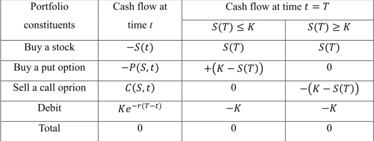
Proposition 2.1: European put-call parity at time t for non-dividend paying stock is
𝑃(𝑆, 𝑡) + 𝑆(𝑡) = 𝐶(𝑆, 𝑡) + 𝐾𝑒 ( ),
where 𝑃(𝑆, 𝑡) is the European put option price with strike price 𝐾 and maturity 𝑇;;
𝐶(𝑆, 𝑡) is the corresponding European call option price;; 𝑆(𝑡) is the underlying share price at time t.
Proof: Construct the following trading strategy as a portfolio:
· Buy one unit of the underlying asset with price 𝑆(𝑡) at time 𝑡 and sell it back at time T with price 𝑆(𝑇).
· Buy a European put option with strike K and expiration T, pay option price 𝑃(𝑆, 𝑡) at time 𝑡 and keep to maturity.
· Sell a European call option with strike K and expiration T and keep to maturity.
· Borrow cash amount 𝐾𝑒 ( ) with continuously compounded interest rate r at time 𝑡, repay K at time T.
Portfolio constituents
Cash flow at time t
Cash flow at time 𝑡 = 𝑇 𝑆(𝑇) ≤ 𝐾 𝑆(𝑇) ≥ 𝐾
Buy a stock −𝑆(𝑡) 𝑆(𝑇) 𝑆(𝑇)
Buy a put option −𝑃(𝑆, 𝑡) + 𝐾 − 𝑆(𝑇) 0
Sell a call oprion 𝐶(𝑆, 𝑡) 0 − 𝐾 − 𝑆(𝑇)
Debit 𝐾𝑒 ( ) −𝐾 −𝐾
Total 0 0 0
Table 2.2.4 Cash flow of portfolio It is interesting to observe that:
Cash flow at time T: max(𝑆(𝑇) − 𝐾, 0) − max(𝐾 − 𝑆(𝑇), 0) + 𝑆(𝑇) − 𝐾 = 0.
According to no-arbitrage argument, cash flow at time t should be equal to the cash flow at time 𝑇. It gives that cash flow at 𝑡 equals zero. Hence, we have:
Cash flow at time t: −𝑆(𝑡) − 𝑃(𝑆, 𝑡) + 𝐶(𝑆, 𝑡) + 𝐾𝑒 ( ) = 0.
Thus,
𝑃(𝑆, 𝑡) + 𝑆(𝑡) = 𝐶(𝑆, 𝑡) + 𝐾𝑒 ( ).
2.2.4 Bounds on prices of European options
Proposition 2.2: Upper bound on the price of a European call/put option price at time 𝑡 are
𝐶(𝑆, 𝑡) ≤ 𝑆(𝑡) for call options,
𝑃(𝑆, 𝑡) ≤ 𝐾𝑒 ( ) for put options.
Proof: Since the European call option gives the buyer the right to buy one share of underlying asset for a certain price, the option can never be worth more than the asset. Hence, we have
For a European put option, the option price at the maturity cannot be worth more than strike price K, it means that the European put option price cannot be worth more than the present value of K today.
Hence, we have
𝑃(𝑆, 𝑡) ≤ 𝐾𝑒 ( ).
Proposition 2.3: Lower bound for a European call/put option price are
𝐶(𝑆, 𝑡) ≥ max {𝑆(𝑡) − 𝐾𝑒 ( ), 0} for call options,
𝑃(𝑆, 𝑡) ≥ max {𝐾𝑒 ( )− 𝑆(𝑡), 0} for put options. Proof: Using put-call parity, we have:
𝐶(𝑆, 𝑡) = max 𝑃(𝑆, 𝑡) + 𝑆(𝑡) − 𝐾𝑒 ( ), 0 ≥ max {𝑆(𝑡) − 𝐾𝑒 ( ), 0}.
𝑃(𝑆, 𝑡) = max 𝐶(𝑆, 𝑡) + 𝐾𝑒 ( )− 𝑆(𝑡), 0 ≥ max { 𝐾𝑒 ( )− 𝑆(𝑡), 0}.
3 Models
Option pricing models are systematic mathematical approaches (closed form formulas, partial differential equation problems or a system of equations with restrictive conditions) that can be used to calculate a theoretical value for financial option contracts. The most widely known work for valuing financial options with a closed mathematical formula is by Black and Scholes (1973) who established the so-called Black-Scholes formula. After the B-S formula, several other approaches were proposed (for example, Garman, 1976;; Cox, Ingersoll and Ross, 1985, p. 379) incorporating different features or assumptions on option pricing.
In this chapter we introduce some of these option pricing models. In Section 3.1, we study the Black-Scholes equation and the corresponding closed form solution (Black and Scholes, 1973). In Section 3.2, we consider stochastic volatility and introduce the Hull-White (H-W) model (Hull and White, 1987) and the Heston model (Heston, 1993). Subsequently we present some numerical methods (binomial methods and finite difference methods) for computing option prices.
3.1 Black-Scholes option pricing model
In this section, Black-Scholes differential equation (Black and Scholes, 1973) and the corresponding closed form solutions are presented.
3.1.1 Black-Scholes model
To derive the Black-scholes option value formula (Black and Scholes, 1973), we make the following assumptions:
· The interest rate is a known constant through time.
· The instantaneous log return of the stock price is an infinitesimal random walk with drift;; more precisely, it is a geometric Brownian motion, and it is assumed that its drift 𝜇 and volatility 𝜎 are constants.
· The option is a European option, that is, it can only be exercised at maturity.
· There is no arbitrage opportunity.
· It is possible to borrow and lend any amount, even fractional, of cash at the riskless rate. It is possible to buy and sell any amount, even a fraction of a share of the underlying stock. There are no transaction fees and taxes.
Under these assumptions, the value of the European option depends only on the stock price, strike price and time to maturity.
Assume that S is the stock price. Suppose that the stock price follows a geometric Brownian motion, as described by (2.1.4) we have
𝑑𝑆(𝑡) = 𝜇𝑆(𝑡)𝑑𝑡 + 𝜎𝑆(𝑡)𝑑𝑊(𝑡),
where 𝜇 is the constant drift of the asset returns, and 𝜎 is the constant volatility of the asset returns.
Suppose V is the value of the financial option with strike price K and maturity T, which is a function of the underlying asset price S and time t, 𝑉(𝑆, 𝑡). From Ito’s formula, we
have 𝑑𝑉 =𝜕𝑉 𝜕𝑡 𝑑𝑡 + 𝜕𝑉 𝜕𝑆𝑑𝑆 + 1 2𝜎 𝑆 𝜕 𝑉 𝜕𝑆 𝑑𝑡, 0 < 𝑆 < ∞, 0 < 𝑡 < 𝑇, (3.1.1)
In the following, we follow the argument of Hull (2009, p. 287). Construct a portfolio F by buying a unit of V and selling (short) units of S
𝐹 = 𝑉(𝑆, 𝑡) − 𝜃𝑆, (3.1.2)
According to Hull (2009, p. 287), we obtain,
𝑑𝐹 = 𝑑𝑉 − 𝜃𝑑𝑆, combine with (3.1.1), it implies
𝑑𝐹 =𝜕𝑉 𝜕𝑡 𝑑𝑡 + 𝜕𝑉 𝜕𝑆𝑑𝑆 + 1 2𝜎 𝑆 𝜕 𝑉 𝜕𝑆 𝑑𝑡 − 𝜃𝑑𝑆, 0 < 𝑆 < ∞, 0 < 𝑡 < 𝑇. (3.1.3)
Choose 𝜃, such that F is a riskless asset, that is, F is independent of S, we achieve this by letting
𝜕𝑉 𝜕𝑆𝑑𝑆 − 𝜃𝑆 = 0, (3.1.4) in (3.1.3) and obtain 𝜃 =𝜕𝑉 𝜕𝑆. (3.1.5) ⟹ 𝑑𝐹 =𝜕𝑉 𝜕𝑡 𝑑𝑡 + 1 2𝜎 𝑆 𝜕 𝑉 𝜕𝑆 𝑑𝑡. (3.1.6)
In finance, 𝜃 defined by (3.1.5) is the so called delta hedging ratio.
Since the new portfolio F is a riskless asset, it should satisfy , combining this with (3.1.6), we obtain
𝜕𝑉 𝜕𝑡 + 𝑟𝑆 𝜕𝑉 𝜕𝑆+ 1 2𝜎 𝑆 𝜕 𝑉 𝜕𝑆 − 𝑟𝑉 = 0, 0 < 𝑆 < ∞, 0 < 𝑡 < 𝑇. (3.1.7)
This partial differential equation (3.1.7) is called the Black-Scholes partial differential equation or Black-Scholes equation for short. We make three remarks about this equation (Wilmott, Howison & Dewynne, 1995):
· The Black-Scholes equation (3.1.7) is a linear backward parabolic partial differential
equation.
· The delta hedging ratio given by (3.1.5) is the rate of change of the value of the
option with respect to the underlying asset price S.
· The Black-Scholes equation (3.1.7) does not contain the growth rate 𝜇 of the underlying share.
The next step is to solve the Black-Scholes equation (3.1.7) and obtain solutions for the
European call and put options.
3.1.2 Formulas for the European call and put options prices For European call options, we have the equation
𝜕𝐶 𝜕𝑡 + 𝑟𝑆 𝜕𝐶 𝜕𝑆+ 1 2𝜎 𝑆 𝜕 𝐶 𝜕𝑆 − 𝑟𝐶 = 0, 0 < 𝑆 < ∞, 0 < 𝑡 < 𝑇, (3.1.8) dF=rFdt
where 𝐶(𝑆, 𝑡) is the value of the European call option with strike price K and maturity T. The final condition for Equation (3.1.8) is
𝐶(𝑆, 𝑇) = 𝑆 − 𝐾, 𝑖𝑓 𝑆 > 𝐾, 0 < 𝑆 < ∞
0, 𝑖𝑓 𝑆 ≤ 𝐾, 0 < 𝑆 < ∞. (3.1.9)
And the boundary condition is
𝐶(0, 𝑡) = 0, 0 < 𝑡 < 𝑇
𝐶(𝑆, 𝑡) ~ 𝑆, 𝑎𝑠 𝑆 → ∞, 0 < 𝑡 < 𝑇. (3.1.10)
According to the final condition in (3.1.9) and the boundary condition in (3.1.10), the equation (3.1.8) can be explicitly solved (e.g. Wilmott, Howison & Dewynne, 1995) and the explicit solution is called the B-S pricing formula for European call options:
𝐶(𝑆, 𝑡) = 𝑁(𝑑 )𝑆 − 𝑁(𝑑 )𝐾𝑒 ( ), (3.1.11) with 𝑑 = 1 𝜎√𝑇 − 𝑡 𝑙𝑛 𝑆 𝐾 + 𝑟 + 𝜎 2 (𝑇 − 𝑡) , 𝑑 = 𝑑 − 𝜎√𝑇 − 𝑡, (3.1.12)
where 𝑁(∙) is the cumulative distribution function of the standard normal distribution. For European put options, the Black-Scholes equation (3.1.7) becomes
𝜕𝑃 𝜕𝑡 + 𝑟𝑆 𝜕𝑃 𝜕𝑆+ 1 2𝜎 𝑆 𝜕 𝑃 𝜕𝑆 − 𝑟𝑃 = 0, 0 < 𝑆 < ∞, 0 < 𝑡 < 𝑇, (3.1.13)
where 𝑃(𝑆, 𝑡) is the value of a European put option with strike price K and maturity T. We have the final condition for equation (3.1.13)
𝑃(𝑆, 𝑇) = 𝐾 − 𝑆, 𝑖𝑓 𝑆 < 𝐾, 0 < 𝑆 < ∞
0, 𝑖𝑓 𝑆 ≥ 𝐾, 0 < 𝑆 < ∞. (3.1.14)
And the boundary conditions
𝑃(0, 𝑡) = 𝐾𝑒 ( ), 0 < 𝑡 < 𝑇
𝑃(𝑆, 𝑡) ~ 0, 𝑎𝑠 𝑆 → ∞, 0 < 𝑡 < 𝑇. (3.1.15)
Solving (cf. Wilmott, Howison & Dewynne, 1995) the equation in (3.1.13) with the final condition in (3.1.14) and the boundary condition in (3.1.15), we obtain
where 𝑑 , are the same as (3.1.12) .
3.2 Stochastic volatility models
Two typical stochastic volatility models will be introduced in this section. The first is Hull-White stochastic model (Hull and White, 1987), whilst the second is the Heston model (Heston, 1993). In this section, we only study the concepts of the models. Because explicit solutions are no longer available as in Black-Scholes case, the Monte
-Carlo simulations for both models are presented in Section 4.
3.2.1 Hull-White stochastic model
Hull and White (1987) considered a derivative asset 𝑓 with a price that depends upon some security price 𝑆, time to maturity 𝑇, and its instantaneous variance, 𝑉 = 𝜎 , which are assumed to obey the following stochastic processes:
𝑑𝑆(𝑡) = 𝜇𝑆(𝑡)𝑑𝑡 + 𝜎(𝑡)𝑆(𝑡)𝑑𝑊 (𝑡), (3.2.1)
𝑑𝑉(𝑡) = 𝜑𝑉(𝑡)𝑑𝑡 + 𝜉𝑉(𝑡)𝑑𝑊 (𝑡), (3.2.2) The variable 𝜇 is dependent on S, and t. The variables 𝜑 and 𝜉 depend on 𝜎 and t. 𝑑𝑊 and 𝑑𝑊 are Brownian motions/ Wiener processes and they are correlated with the correlation coefficient 𝜌.
There are several assumptions for Hull-White model:
· The volatility 𝑉 is uncorrelated with the stock price S.
· 𝑆, 𝑇 and 𝜎 are the only state variables which affect the price of the derivative security 𝑓.
· The risk-free rate, 𝑟, must be a constant or at least deterministic.
3.2.2 Heston model
The Heston model (Heston, 1993) assumes that the stock price 𝑆(𝑡) and its instantaneous variance 𝑉(𝑡) satisfy the following stochastic differential equations (SDEs):
𝑑𝑉(𝑡) = −𝜆(𝑉(𝑡) − 𝜃)𝑑𝑡 + 𝜂 𝑉(𝑡)𝑑𝑊 (𝑡), (3.2.4) ⟨𝑑𝑊 , 𝑑𝑊 ⟩ = 𝜌𝑑𝑡. (3.2.5) The parameters in the above equations represent the following:
· 𝜇 is the drift coefficient of stock price returns
· 𝜃 is the long-term mean of price variance
· 𝜆 is the speed of reversion of 𝑉(𝑡) to its long-term mean 𝜃
· 𝜂 is the volatility of volatility
· 𝜌 is the correlation between Brownian motions
· 𝑑𝑊 and 𝑑𝑊 are Brownian motions/ Wiener processes and they are correlated with the correlation coefficient 𝜌
This process (3.2.3) uses the instantaneous variance 𝑉(𝑡), which is defined by the theory proposed in Cox, Ingersoll and Ross (1985, p.399). It is usually referred to as CIR process.
There are two assumptions for the Heston model (Heston, 1993):
· The interest rate is constant.
· There is no dividend payment.
3.3 Numerical methods
3.3.1 Binomial methods
Using discrete random walk models, we attempt to emulate the price movement of the underlying asset. Once the movement pattern of the underlying asset is set, we can use this pattern to price the derived option price. If the random walk consists of two possibilities, one is up and the other is down, then the model is a binomial model and the method is classified as binomial method. There are two assumptions (Wilmott, Howison and Dewynne, 1995) underlying the binomial methods:
· Suppose that the lifetime of the option is 𝑇, which is divided up into 𝑀 time-steps of size ∆𝑡 = 𝑇/𝑀. The continuous random walk can be approximately utilised by a discrete random walk. The asset price 𝑆 changes only at the discrete times
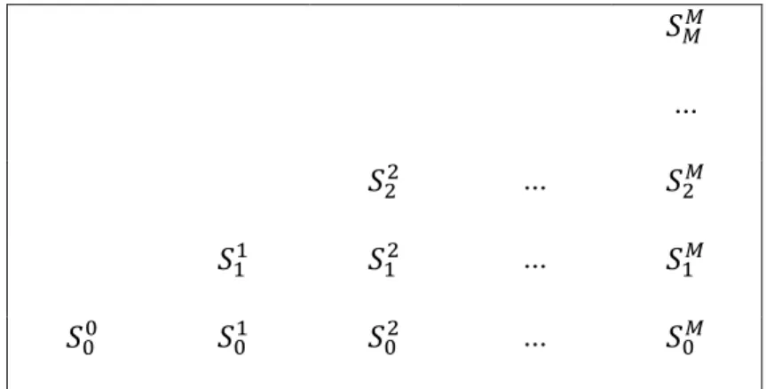
∆𝑡, 2∆𝑡, . . . , 𝑀∆𝑡 = 𝑇. We suppose that the asset price is 𝑆 at time 𝑡 = 𝑚∆𝑡, then the asset price at time 𝑡 = (𝑚 + 1) ∆𝑡, has two possibilities: moving up to 𝑢𝑆 with probability 𝑝 (0 < 𝑝 < 1) or moving down to 𝑑𝑆 with probability 1 – 𝑝 (𝑢 > 1 > 𝑑 > 0). The binomial tree is constructed by starting with the given value 𝑆, which is the asset price at 𝑡 = 0, generating two possible asset prices at the first time step 𝑡 = ∆𝑡, three possible values at the second time step 𝑡 = 2∆𝑡 until the maturity time of the security. Consequently at time 𝑡 = 𝑚∆𝑡, there are 𝑚 + 1 possibilities for asset prices. Suuu Suu Su Suud S Sud Sd Sudd Sdd Sddd Figure 3.3.1 Binomial tree
· Assume it is a risk-neutral world (Wilmott, Howison & Dewynne, 1995) and thus the stochastic differential equation (2.1.4) is replaced by
𝑑𝑆(𝑡)
𝑆(𝑡) = 𝑟𝑑𝑡 + 𝜎𝑑𝑊(𝑡), (3.3.1)
where 𝑟 is the risk-free interest rate.
With these assumptions, we observe that the option value 𝑉 at time 𝑡 = 𝑚∆𝑡 is the expected value of the option value at time 𝑡 = (𝑚 + 1) ∆𝑡, discounted by the risk-free interest rate 𝑟.
𝑉 = 𝐸[𝑒 ∆ 𝑉 ]. (3.3.2) Choosing the probability 𝑝 of asset price moving up and 1 – 𝑝 of asset price moving down, the moving up magnitude 𝑢 and moving down magnitude 𝑑 is such that the
discrete random walk presented by the binomial tree and the continuous random walk (3.3.1) have the same mean and variance (Wilmott, Howison and Dewynne, 1995). This means that the expected values and variances of a time-step under the continuous risk-neutral random walk (3.3.1) and the discrete binomial model are equal.
We have the expected value and the variance of 𝑆 , given 𝑆 , under the continuous random walk (3.3.1):
𝐸 [𝑆 |𝑆 ] = ∫ 𝑆 𝑝(𝑆 , 𝑚∆𝑡; 𝑆 , (𝑚 + 1)∆𝑡) 𝑑𝑆 = 𝑒 ∆ 𝑆 , (3.3.3)
𝑉𝑎𝑟 [𝑆 |𝑆 ] = 𝑒 ∆ (𝑒 ∆ − 1)(𝑆 ) , (3.3.4)
where 𝑝(𝑆, 𝑡; 𝑆 , 𝑡 ) is the probability density function
𝑝(𝑆, 𝑡; 𝑆 , 𝑡 ) =
( )𝑒
( / ) ( )( ) / ( ), (3.3.5)
for the risk-neutral random walk (3.3.1) (Wilmott, Howison & Dewynne, 1995). For the discrete binomial random walk, the expected value of 𝑆 under 𝑆 is
𝐸 [𝑆 |𝑆 ] = (𝑝𝑢 + (1 − 𝑝)𝑑)𝑆 , (3.3.6) 𝑉𝑎𝑟 [𝑆 |𝑆 ] = (𝑝𝑢 + (1 − 𝑝)𝜎 − 𝑒 ∆ )(𝑆 ) . (3.3.7)
Let 𝐸 [𝑆 |𝑆 ] = 𝐸 [𝑆 |𝑆 ], 𝑉𝑎𝑟 [𝑆 |𝑆 ] = 𝑉𝑎𝑟 [𝑆 |𝑆 ], we obtain,
𝑝𝑢 + (1 − 𝑝)𝑑 = 𝑒 ∆ , (3.3.8) 𝑝𝑢 + (1 − 𝑝)𝜎 = 𝑒( )∆ . (3.3.9)
For the three unknown values 𝑢, 𝑑 and 𝑝, we have two equations (3.3.8) and (3.3.9). We require three equations to determine three unknown values. Hence, we need another equation. The choice of the third equation is somewhat arbitrary. Two frequently selected options for the third equation are:
𝑢 = , (3.3.10) or
In the case of (3.3.10), the unknown values 𝑢, 𝑑 and 𝑝 are determined by the equations (3.3.8), (3.3.9) and (3.3.10). We obtain
𝑢 = 𝐴 + 𝐴 − 1, 𝑑 = 𝐴 − 𝐴 − 1, 𝑝 =𝑒 ∆− 𝑑
𝑢 − 𝑑 , (3.3.12)
where 𝐴 = 𝑒 + 𝑒( )∆ .
Since 𝑢 = , 𝑆𝑢𝑑 in Figure 3.3.1 becomes 𝑆. It is easy to observe that the binomial tree is vertically symmetrical.
Suppose the asset price at the beginning time is 𝑆 = 100, 𝑢 = = , the binomial tree is shown in Figure 3.3.2.
244 195 156 156 125 125 100 100 100 80 80 64 64 51 41
Figure 3.3.2: Binomial tree of underlying asset price when 𝑢 =
In the case of (3.3.11), the unknown values 𝑢, 𝑑 and 𝑝 are determined by the equations (3.3.8), (3.3.9) and (3.3.11). We obtain
𝑢 = 𝑒 ∆ 1 + 𝑒 ∆ − 1 , 𝑑 = 𝑒 ∆ 1 − 𝑒 ∆ − 1 , 𝑝 =1
2. (3.3.13)
Only if 𝑢 ∙ 𝑑 = 1, 𝑆𝑢𝑑 = 𝑆. In general, the binomial tree will be slightly upwardly adjusted if 𝑢 ∙ 𝑑 > 1, or downwardly adjusted if 𝑢 ∙ 𝑑 < 1.
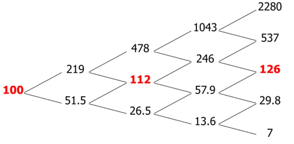
Let 𝑝 = 0.5, 𝑟 = 0.2, ∆𝑡 = 1, 𝜎 = 0.2. We have 𝑢 = 1.9772, 𝑑 = 0.4656, 𝑢 ∙ 𝑑 ≈ 0.9206 < 1. With asset price 𝑆 = 100 at the beginning, according to the above discussion about 𝑢 ∙ 𝑑 < 1, we have a downwardly adjusted binomial tree which is shown in Figure 3.3.3.
1528 773 391 198 360 100 182 92.1 46.6 84.7 42.9 21.7 20 10.1 4.7
Figure 3.3.3: Binomial tree of underlying asset price when 𝑝 = and 𝑢 ∙ 𝑑 < 1. Let 𝑝 = 0.5, 𝑟 = 0.3, ∆𝑡 = 1, 𝜎 = 0.2. We have 𝑢 = 2.1851, 𝑑 = 0.5146, 𝑢 ∙ 𝑑 ≈ 1.1244 > 1. With asset price 𝑆 = 100 at the beginning, according to the above discussion about 𝑢 ∙ 𝑑 > 1, we have a upwardly adjusted binomial tree which is shown in Figure 3.3.4. 2280 1043 537 478 246 219 126 112 100 57.9 51.5 29.8 26.5 13.6 7
Figure 3.3.4: Binomial tree of underlying asset price when 𝑝 = and 𝑢 ∙ 𝑑 > 1.
3.3.2 Pricing European option with binomial methods
Suppose 𝑉 is the value of the European put option at 𝑡 = 𝑇 = 𝑀∆𝑡, and the payoff function for the option depends only on the values of the underlying asset at maturity. The value of the European put option at the maturity can be priced as:
where 𝑉 is the 𝑛-th possible value of the European put option at time-step 𝑀, 𝐾 is the strike price and 𝑆 denotes the 𝑛-th possible value of the underlying asset at time-step
𝑀.
Since we have the binomial tree of the underlying asset price (Figure 3.3.1), we can calculate all values of 𝑆 , 𝑛 = 0, 1, … , 𝑚, 𝑚 = 0, 1, … , 𝑀 and the corresponding probability 𝑝 which represents the probability of 𝑆 moving up to 𝑆 and the probability 1 − 𝑝 which is the probability of 𝑆 moving down to 𝑆 .
With the option price and the prices of underlying assets at maturity, we can calculate the expected value of the option at the time-step prior to the maturity (𝑀 − 1)∆𝑡 by discounting the values of maturity with the risk-free interest rate 𝑟.
𝑒 ∆ 𝑉 = 𝑝𝑉 + (1 − 𝑝)𝑉 , 0 ≤ 𝑛 ≤ 𝑀 − 1,
for the time-step 𝑚∆𝑡, 0 ≤ 𝑚 < 𝑀, we have
𝑒 ∆ 𝑉 = 𝑝𝑉 + (1 − 𝑝)𝑉 , 0 ≤ 𝑚 < 𝑀, 0 ≤ 𝑛 ≤ 𝑚. (3.3.15)
This gives
𝑉 = 𝑒 ∆ (𝑝𝑉 + (1 − 𝑝)𝑉 ), 0 ≤ 𝑚 < 𝑀, 0 ≤ 𝑛 ≤ 𝑚. (3.3.16)
We can calculate the values of 𝑉 for each 𝑛 and 𝑚, at last arriving at the current option price 𝑉 . 𝑆 ... 𝑆 ... 𝑆 𝑆 𝑆 ... 𝑆 𝑆 𝑆 𝑆 ... 𝑆
𝑉 𝑚𝑎𝑥(𝐾 − 𝑆 , 0) ... 𝑉 𝑒 ∆(𝑝𝑉 + (1 − 𝑝)𝑉 ) ... 𝑉 𝑚𝑎𝑥(𝐾 − 𝑆 , 0) 𝑉 𝑒 ∆(𝑝𝑉 + (1 − 𝑝)𝑉 ) 𝑉 𝑒 ∆(𝑝𝑉 + (1 − 𝑝)𝑉 ) ... 𝑉 𝑚𝑎𝑥(𝐾 − 𝑆 , 0) 𝑉 𝑒 ∆(𝑝𝑉 + (1 − 𝑝)𝑉 ) 𝑉 𝑒 ∆(𝑝𝑉 + (1 − 𝑝)𝑉 ) 𝑉 𝑒 ∆(𝑝𝑉 + (1 − 𝑝)𝑉 ) ... 𝑉 𝑚𝑎𝑥(𝐾 − 𝑆 , 0) Figure 3.3.3: The binomial tree of European put option price
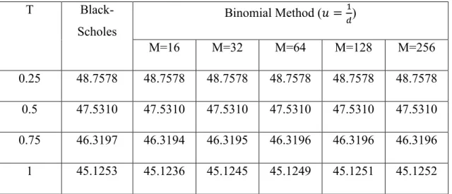
We simulate the option pricing process using both (3.3.12) and (3.3.13) with different time to maturity and time steps. Thereafter researchers can compare the B-S option price with the price calculated by binomial option pricing methods (Table 3.3.1 and Table 3.3.2). T Black -Scholes Binomial Method (𝑝 = ) M=16 M=32 M=64 M=128 M=256 0.25 48.7578 48.7578 48.7578 48.7578 48.7578 48.7578 0.5 47.5310 47.5310 47.5310 47.5310 47.5310 47.5310 0.75 46.3197 46.3195 46.3195 46.3196 46.3196 46.3196 1 45.1253 45.1241 45.1246 45.1249 45.1252 45.1253
Table 3.3.1 Comparison of Black-Scholes values and binomial method (𝑝 = ) for a European put option with 𝐾 = 100, 𝑆 = 50, 𝑟 = 0.05, and 𝜎 = 0.2. Expiry time T is measured in years.
T Black -Scholes Binomial Method (𝑢 = ) M=16 M=32 M=64 M=128 M=256 0.25 48.7578 48.7578 48.7578 48.7578 48.7578 48.7578 0.5 47.5310 47.5310 47.5310 47.5310 47.5310 47.5310 0.75 46.3197 46.3194 46.3195 46.3196 46.3196 46.3196 1 45.1253 45.1236 45.1245 45.1249 45.1251 45.1252
Table 3.3.2 Comparison of Black-Scholes values and binomial method (𝑢 = ) for a European put option with 𝐾 = 100, 𝑆 = 50, 𝑟 = 0.05, and 𝜎 = 0.2. Expiry time T is measured in years.
4 Simulation and regression
In this chapter we present the methods used to analyse the real market data. Boyle (1977, p. 329) and Boyle, Broadie, and Glasserman (1997, p. 1268) utilized Monte
-Carlo simulation in derivative pricing and Michael, Fu and Laprise (1999, p. 57) conducted empirical testing to compare the different algorithms. We revisit Monte-Carlo simulation to explore how this method can be used for pricing options in Section 4.1. In Section 4.1, we apply Monte-Carlo simulation in pricing European options, using a standard random walk model, the Hull-White model and the Heston model for the underlying stock prices. We compare the results using Monte-Carlo simulation with the Black-Scholes price obtained using the Black-Scholes formula. In Section 4.2, the regression method will be introduced.
4.1 Monte-Carlo simulation for pricing European options
Monte-Carlo simulation is one of the mathematical methods for pricing financial derivatives. Here we give three examples to understand the application of Monte-Carlo simulation on pricing European options.4.1.1 Monte-Carlo simulation using standard Brownian model
Firstly, we use the standard random walk model to simulate the underlying asset price. We assume that the stock has no dividends and the price follows a geometric Brownian motion (cf. (2.1.4)):
𝑑𝑆(𝑡) = 𝜇𝑆(𝑡)𝑑𝑡 + 𝜎𝑆(𝑡)𝑑𝑊(𝑡), for 𝑡 > 0.
Here is the stock price at time t, W is a Brownian motion, 𝜇 is the assumed constant drift, 𝜎 is the assumed constant volatility.
The solution of the geometric Brownian motion is (cf. (2.1.5)):
𝑆(𝑡) = 𝑆 exp 𝜇 − 𝑡 + 𝜎𝑊(𝑡) . If we rewrite the above equation as a discrete time process:
𝑆(𝑡 + ∆𝑡) = 𝑆(𝑡)exp 𝜇 − 𝑡 + 𝜎𝜀(𝑡)√∆𝑡 , (4.1.1)