Why do Differences in the Degree of Fiscal
Decentralization Endure?
Xavier Calsamiglia
Department of Economics and Business Universitat Pompeu Fabra
Teresa Garcia-Mil`a
Department of Economics and Business Universitat Pompeu Fabra
Therese J. McGuire
Management and Strategy Department Kellogg School of Management
Northwestern University and
Institute for Policy Research Northwestern University ∗ Preliminary version: August 21, 2004
∗Contact information: Xavier Calsamiglia, Department of Economics and
Busi-ness, Universitat Pompeu Fabra, Ramon Trias Fargas 25-27, 08005 Barcelona, Spain, [email protected]. Teresa Garcia-Mil`a, Department of Economics and Busi-ness, Universitat Pompeu Fabra, Ramon Trias Fargas 25-27, 08005 Barcelona, Spain, [email protected]. Therese J. McGuire, Management and Strategy Department, Kellogg School of Management, Northwestern University, 2001 Sheridan Road, Evanston IL 60208, USA, [email protected]
1 Introduction
A notable difference between the U.S. and many countries in Europe is in the degree of fiscal decentralization. Regional (and local) governments in the U.S. have significant autonomy in setting their own taxes and determining how to spend their revenues. This is not true of their counterparts in Spain, France, the United Kingdom, Czech Republic and many other European countries. In recent years, many countries formerly subject to dictatorships or communism have been considering decentralizing fiscal responsibility to sub-national governments as part of the process of democratization (see Bird and Ebel, forthcoming). Yet, much of Europe remains immune to adopting effective decentralization in which sub-national units have true taxing authority.
As Oates (1972, 1999) has argued, there can be significant efficiency gains to having a federal system with fiscally empowered sub-national levels of government. On the other hand, such systems typically result in a lack of uniformity in public good provision as sub-national units of government with varying tastes and varying levels of income choose diverging types and quantities of public goods. Garcia-Mil`a and McGuire (forthcoming) postu-late a model in which people can have a preference for uniformity in public good provision across regions, what the authors call solidarity. They find that, in countries where this is true, relatively rich regional governments will voluntarily redistribute resources to relatively poor regional governments.
In the present paper, we argue that differences across countries in prefer-ences for equality in provision of regional public goods can lead to dissimilar choices over the degree of fiscal decentralization. In simulations, we show that a decentralized system may Pareto dominate a centralized system if preferences for regional solidarity are weak, and the opposite holds if soli-darity preferences are strong. Thus, according to our model, it is possible for a decentralized system to be optimal for the U.S. but inappropriate for Europe.
In the next section, we characterize and evaluate the normative quali-ties of three stylized systems of fiscal federalism: a completely centralized model, a completely decentralized model, and a model in between these two extremes in which the central government finances a minimum amount of public expenditure, and regional governments have the ability to tax them-selves to spend more. In section 3, we simulate outcomes under the three systems, altering the preferences for solidarity from weak to strong. In sec-tion 4, we present some empirical facts that appear to be consistent with the theory and simulation results. We conclude in section 5.
2 A theory of fiscal decentralization with regional solidarity
We specify a model with a central government andnregional governments. The regions have initial wealth ωi. Let ω = Pnj=1ωj be the aggregate wealth. There are two commodities: private consumption, ci, and public
expenditure,gi. Both are private goods.
We assume that all regions are concerned with inequalities in public expenditures, as measured by the inequality index
e= 1 n n X j=1 (gj−g¯)2 where g¯= 1 n n X j=1 gj
Preferences of thei-th region are representable by a concave utility func-tionui(ci, gi, e), where ∂ui ∂ci >0 ∂ui ∂gi >0 ∂ui ∂e <0
A Pareto optimal allocation is necessarily a solution of the following problem: choose the private consumption and public expenditure levels (ci, gi) for i∈ {1,2, . . . , n}that solve the problem:
max n X j=1 αjuj(cj, gj, e) (1) s.t. n X j=1 cj+ n X j=1 gj = n X j=1 ωj (2) ci ≥0 i∈ {1,2, . . . , n} (3) gi ≥0 i∈ {1,2, . . . , n} (4)
By choosing different weights, αi > 0, all possible Pareto optimal
allo-cations are generated. The first order necessary conditions for this problem are therefore necessary conditions for Pareto optimality.
The Lagrangian expression for this problem is
L(c1, c2, . . . , cn, g1, g2, . . . , gn, λ) = n X j=1 αjuj(cj, gj, e)−λ n X j=1 (cj +gj)− n X j=1 ωj
The Kuhn-Tucker first order necessary conditions are: ∂L ∂ci = αi ∂ui ∂ci −λ≤0 i∈ {1,2, . . . , n} (5) ∂L ∂gi = αi ∂ui ∂gi + n X j=1 αj ∂uj ∂e ∂e ∂gi −λ≤0 i∈ {1,2, . . . , n} (6) Each of these inequalities must hold with equality if we have interior solutions ci > 0 and gi > 0. In the case of interior solutions, from the
preceding equalities we get:
αi ∂ui ∂ci = αj ∂uj ∂cj ∀i, j (7) αi ∂ui ∂gi + 2 n(gi−¯g) n X k=1 αk ∂uk ∂e = αj ∂uj ∂gj + 2 n(gj−¯g) n X k=1 αk ∂uk ∂e ∀i, j(8) αi ∂ui ∂ci = αj ∂uj ∂gj + 2 n(gj−¯g) n X k=1 αk ∂uk ∂e ∀i, j(9) Equation (7) requires that the marginal contributions of private con-sumption to social welfare is the same in all regions. Equation (8) requires the equality of the marginal contributions of public expenditure to social welfare in all regions. Finally, equation (9) establishes that the marginal contribution to social welfare of private consumption equals that of public expenditure in all regions.
As can be seen in the right hand side of (8), the marginal contribution to social welfare of public expenditure in regionihas two components: the direct effect,αi∂u∂gii, and the indirect effect ofgion all region’s welfare through
e 2 n(gi−¯g) n X k=1 αk ∂uk ∂e (10)
If all public expenditures are equalized, then gi = ¯g and the indirect
effect disappears.
We next present and characterize the choices made under three different systems of fiscal federalism:
a) Complete centralization: In this model, the central government
im-poses a uniform tax system to raise funds for provision of a uniform level of publicly provided private good across the country.
b) Complete decentralization: In this model, local governments have tax-ing authority and revenue-raistax-ing responsibility. They are free to set the level of the publicly provided private good without any interfer-ence (or assistance) from the central government. They can decide to make voluntary contributions to other local governments to help them increase their public expenditures.
c) Guaranteed minimum level: The central government imposes a
uni-form tax system to raise funds for a central grant to regions that supports a minimal (adequate) level of the publicly provided private good in each region. Regions have local taxing authority that they can employ to adjust the spending levels above the minimal required level.
We compare the outcome for each system to the Pareto optimality con-ditions.
2.1 Centralized financing of regional governments
Under this system, the only source of funding for public expenditure is a transfer, si, from the central government. There is no local power to tax,
nor the possibility of increasing private consumption by using subsidies from the central government. Hencegi =si.
The central government has acommon tax function for all regional gov-ernments. The tax function is increasing in income or even progressive but cannot discriminate by region of residence. To simplify the analysis we as-sume a proportional tax, φ(ω) =tω, where t ∈ [0,1] is the tax rate. The crucial assumption is thattis the same for all local governments.
Given some welfare weights, αi, the central government has to find
t ∈ [0,1] and a vector of transfers, or equivalently public expenditures, (g1, g2, . . . , gn), that solve the problem
max n X j=1 αjuj(cj, gj, e) (11) s.t. n X j=1 gj =t n X j=1 ωj (12) ci= (1−t)ωi i∈ {1,2, . . . , n} (13) gi ≥0 i∈ {1,2, . . . , n} (14) 0≤t≤1 (15)
Local governments do not have decision power: public expenditure is de-cided at the central level and private consumption is just a residual variable, ci= (1−t)ωi, since it equals the after tax wealth. If there is decentralization
at all, it is just an “administrative decentralization”.
Recall that public expenditure is a private good that could be efficiently provided by local governments. The only reason for central government in-tervention is the existence of solidarity. We thus assume that the central government provides equal subsidies to all regions, s = si. Consequently,
public expenditures are equalized across regions, gi =g. In the completely
centralized system the central government has two constraints: the tax func-tion cannot discriminate across regions and public expenditures should be equalized.
The maximization problem (11−15) can be simplified to
max n X j=1 αjuj((1−t)ωj, g, e) (16) s.t. ng=t n X j=1 ωj (17) g≥0 i∈ {1,2, . . . , n} (18) 0≤t≤1 (19)
The Lagrangian expression for this problem is
L(t, g, λ) = n X j=1 αj(uj(1−t)ωj, g, e)−λ ng−t n X j=1 ωj
Notice that, according to (10), when all public expenditures are equal, gi = g = ¯g, the indirect effect disappears. In this case, the Kuhn Tucker
first order conditions for a maximum are: ∂L ∂t = − n X j=1 αj ∂uj ∂cj ωj+λ n X j=1 ωj ≤0 (20) ∂L ∂g = n X j=1 αj ∂uj ∂gj −λn≤0 i∈ {1,2, . . . , n} (21)
n X j=1 αj ∂uj ∂cj ωj Pn j=1ωj = 1 n n X j=1 αj ∂uj ∂gj (22) The marginal contribution of public expenditure to social welfare is not necessarily equal to that of private consumption in every region, as required by Pareto optimality in equation (9). Instead, theaverage marginal contri-bution of public expenditure to social welfare is equal to a weighted average of all the region’s marginal contributions of private consumption, the weights being the relative shares of every region in total wealth.
In general, the centralized system leads to inefficient outcomes. The inefficiency arises from the fact that income tax rules cannot discriminate by region of residence and a uniform level of g is chosen by the central government.
2.2 Decentralized decisions by regional governments
Under this system, each regional government has complete freedom of choice of both private consumption and public expenditures. In addition, they can set interregional transfers, sij ≥0, from region ito j which are essentially
voluntary contributions to solidarity. Each regional government choosesgi,
ci and sij (for j 6=i), taking all other variables as given, so as to solve the
following maximization problem
max ui(ci, gi, e) (23) s.t. ci+gi+ X i6=j sij =ωi+ X j6=i sji (24) ci≥0 gi ≥0 sij ≥0 (25)
The Nash equilibrium is obtained by solving simultaneously the n sys-tems of necessary conditions. Setting up the Lagrangian of thei-th region:
L(ci, g1,{sij}j6=i, λi) =ui(ci, gi, e)−λi ci+gi+ X i6=j sij−ωi− X j6=i sji
and taking the first derivatives we obtain: ∂L
∂ci
= ∂ui ∂ci
∂L ∂gi = ∂ui ∂gi +∂ui ∂e ∂e ∂gi −λi ≤0 with equality if gi >0 (27) ∂L ∂sij = ∂ui ∂e ∂e ∂gj
−λi ≤0 with equality if sij >0 forj 6=i (28)
We can make assumptions on the utility function (for instance a Cobb-Douglas type) so thatci and gi are needed in positive amounts in order to
have a positive utility. This would rule out corner solutions. Yet, as we shall see, corner solutions in thesij’s are unavoidable.
Assuming interior solutions forci and gi, from (26) and (27) we get
∂ui ∂ci = ∂ui ∂gi +∂ui ∂e ∂e ∂gi = ∂ui ∂gi + 2 n(gi−¯g) ∂ui ∂e (29)
Again, the marginal contributions ofciandgito i’s utility are equalized,
but the indirect effectdoes not take into account the impact ofgi throughe
on other region’s utilities (as required in equation (9) derived from the first order conditions for a Pareto optimum). Hence, the Nash equilibrium is bound to be inefficient because regions do not take into account the effect of their contributions to other regions’ welfare when setting their interregional transfers. Equality is a public good.
Ifsij >0, then from (26) and (28) we get
∂ui ∂e 2 n(gj−g¯) = ∂ui ∂ci >0 (30)
Notice that, by assumption, ∂ui
∂e < 0 and therefore the interregional
transfer fromito j will only be positive ifgj−g <¯ 0, in other words, ifj is
a region with below average public expenditure.
Moreover, ifsij >0, both (27) and (28) hold with equality and therefore:
∂ui ∂gi + ∂ui ∂e 2 n(gi−g¯) = ∂ui ∂e 2 n(gj−g¯) (31) and since ∂ui
∂gi >0 ∂ui ∂e 2 n(gi−g¯)< ∂ui ∂e 2 n(gj−¯g) (32)
and since ∂ui ∂e <0 2 n(gi−g¯)> 2 n(gj −g¯) (33) and finally gi > gj (34)
that is, a regionisends transfers to regionjifgi > gj andgj <g¯. Obviously,
a corner solution forsij arises when these conditions are not met.
A particular case of the decentralized model that we will discuss later is the autarchy model, where interregional transfers are not allowed (sij =
0 for all i and j) and every region sets its own private consumption and public expenditure levels. Thus, the only way open to local governments to accommodate preferences for solidarity is to readjust their private and public expenditure levels.
2.3 Decentralized decisions with a centrally guaranteed minimum level
We finally consider a mixed model that is a sequential game in which the central government is a Stackelberg leader. In the first stage, the central government sets a common tax ratetfor all regions. The revenue is equally distributed as a subsidysi = s = n1tPnj=1ωj =
t
nω, where ω is aggregate
wealth. This transfer sets up a minimum public expenditure level to all regions. Thei-th’s region total social expenditure isgi+s.
At a later stage, knowing the tax rate and the corresponding subsidy, the regions are free to decide higher public expenditures by raising additional revenue from local taxes. The second phase is modelled as a simultaneous game with the regions as players. The strategic variables are the levels of private consumption,ci, and the locally financed public expenditures,gi ≥0.
Given the value of the central government’s strategic variable,the tax rate t, and taking the values of the other region’s strategic variables as given, the i-th local government choosesci and gi so as to solve
max ui(ci, gi+
t
nω, e) (35)
s.t. ci+gi ≤(1−t)ωi (36)
ci ≥0 gi≥0 (37)
The Lagrangian expression for this problem is:
L(ci, gi, λi) =ui(ci, gi+s, e)−λi(ci+gi−(1−t)ωi)
and taking the first derivatives we obtain the Kuhn-Tucker first order nec-essary conditions: ∂L ∂ci = ∂ui ∂ci −λi≤0 with equality ifci >0 (38) ∂L ∂gi = ∂ui ∂gi +∂ui ∂e ∂e ∂gi −λi ≤0 with equality if gi>0 (39)
Assuming interior solutions forci and gi, from (26) and (27) we get ∂ui ∂ci = ∂ui ∂gi +∂ui ∂e ∂e ∂gi = ∂ui ∂gi + 2 n(gi−¯g) ∂ui ∂e (40)
Again, the marginal contributions ofciandgito i’s utility are equalized,
but the indirect effectdoes not take into account the impact ofgi throughe
on other region’s utilities (as required in equation (9) derived from the first order conditions for a Pareto optimum). Hence, in general,the equilibrium of this game is bound to be inefficient because regions do not take into account the effect of their decisions upon other region’s welfare when setting their strategic variables.
The n equations given by (40), plus the n constraints (one for each region), provide a system of 2n equations with 2n+ 1 unknowns (private consumption and public expenditure levels for every region, plus the tax rate t). By simultaneously solving this system we obtain the region’s reaction functions expressing the optimal responses ci and gi as functions of the
central government’s strategic variable, t. These reaction functions can be plugged-in the central government’s objective function, who then solves the maximization problem max n X j=1 αjuj(cj(t), gj(t), e) (41) s.t. t∈[0,1] (42)
The first order necessary condition for an interior solution requires that the first derivative vanishes:
n X j=1 αj ∂uj ∂cj dcj dt + ∂uj ∂gj dgj dt + ∂uj ∂e de dt = 0
where the derivatives dcj dt ,
dgj
dt and
de
dt can be obtained from the system of
equations (40) by using the implicit function theorem.
As we have seen, in general, the equilibrium of the guaranteed minimum system does not satisfy the first order conditions for Pareto optimality.
3 Simulation results
The results in the theory section can be summarized as follows. When solidarity is present and demands for public expenditure vary by region, then
each fiscal federal system analyzed is inefficient. The centralized solution is inefficient because of the rigidities imposed by a common tax function and a uniform level of public good across all regions. The decentralized solution is inefficient because of the free-rider problems generated by solidarity. Which system dominates will depend on solidarity preferences.
In this section we simulate the systems presented in the previous section to be able to characterize the relationship between solidarity preferences and the degree of decentralization. By comparing a few simulations we confirm that when preferences for equality are strong the centralized system dominates the decentralized one. Similarly, when preferences for equality are weak, decentralization is a superior mechanism.
3.1 The utility function
We consider a very simple multilevel government with two regions. They
haveidentical preferences represented by the utility function
u(ci, gi, e) =K(ci−a)δgiβ
1 1 +γe whereci ≥α, gi ≥0 and eis the variance of{g1, g2}.
The parameter acan be seen as a subsistence level below which private consumption cannot fall. The parameter γ is a nonnegative number cap-turing the strength of the solidarity preferences. When γ = 0 there is no solidarity. To clarify the nature of the class of utility functions, decompose the utility function in two parts: the standard utility, K(ci −a)δgiβ,
rep-resenting preferences between social expenditure and private consumption, and thesolidarity effect, 1
1+γe. When there are no inequalities, the variance
e equals zero and the solidarity effect takes its maximum value, 1. Total utility coincides with the standard utility. When there are inequalities (the varianceeis positive) the solidarity effect is less the one and the total utility is less than the standard utility. The solidarity effect tends to zero as the variance grows to infinity.
The standard utility is a Stone-Geary utility function. When a= 0 it is a Cobb-Douglas function that gives rise to a demand for social expenditure with constant wealth elasticity (η = 1). For positive values of a, demand for social expenditure (taking the relative prices of social expenditure and private consumption equal to unity) is
gi =
δ(ω−a) β+δ
and the wealth elasticity of demand for social expenditure is η= ω
ω−a >1
Hence , for positive values of a, prefereces are not homothetic and give rise to non-linear expenditure systems.
The only difference between the two regions is the wealth level,ω1 = 80 and ω2= 20.
For the simulations that follow we fixa= 10,β = 1,δ= 0.5 andK= 10, so that preferences of all regions are represented by the same utility funtion
u(ci, gi, e) = 10gi(ci−10)
1 1 +γe
We do not assume a particular social welfare function for the central government but rather represent the locus of all utility pairs achievable by choosing different values for the central government’s strategic variables. The following items are represented in the graphs:
a) Utility frontier This is the set of all Pareto optimal utility allocations
satisfying the necessary and sufficient conditions discussed in section 2.
b) Decentralized equilibriumDi, the Nash equilibrium point described in
section 2.2, where every region has the possibility of setting voluntary interregional transfers, together with the level of their own private consumption and public expenditure levels. The central government has no role and local governments have full taxing authority.
c) Autarchy equilibrium, represented by Ai, is the utility vector obtained
when each region independently decides its own levels of public expen-ditures and private consumption, taking into account its preference for solidarity. There is no central government intervention, nor the possi-bility of interregional transfers. It is obtained as a Nash equilibrium with public expenditure levels as strategic variables.
d) Locus of centralized allocations This is the set of all utility allocations that can be attained by a central government that sets taxes and allocates social expenditures equally among the regions as described in section 2.1. The determination of the equilibrium of the centralized model requires the specification of a social welfare function. We find it useful to take as a reference a particular point, Ci, where, in the
Rawlsian tradition, the utility of the poor region is maximized. In our problem this would correspond to the extreme case of a utility function with zero weight, α1 = 0, for the rich region. With other weights, other points of the locus would be selected.
e) Locus of guaranteed minimum Here we consider a mixed system in
which there is a centrally financed guaranteed minimum level of social expenditure, and the regions can complement this with additional local taxes. The locus of guaranteed minimum alllocations describes the set of utility allocations that can be obtained as equilibria of the two stage sequential game described in section 2.3. For every possible tax rate, t ≥ 0, the regions play a simultaneous game. The resulting Nash equilibrium utility payoffs are represented in the locus.
3.2 The no solidarity case
This is the standard case in the literature: whenγ = 0 there is no solidarity effect and we go back to a model with a utility of the form
u(ci, gi, e) =K(ci−a)δgiβ
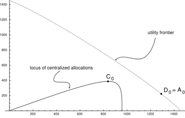
We represent the utility levels attained under the different systems in a graph. Since all goods in our model are private, the decentralized solution, D0, lies on the utility possibility frontier. The optimal voluntary contribu-tions are zero, ¯sij = 0, and consequently, the equilibrium coincides with the
autarchy solution,A0, in which interregional transfers are not allowed.
200 400 600 800 1000 1200 1400 200 400 600 800 1000 1200 1400 utility frontier
locus of centralized allocations
0 C 0 = A 0 D
Under the completely centralized system, the interregional transfer from the rich to the poor equals t
2(ω1 −ω2), so that a higher taxation implies a larger transfer from the rich. The locus of centralized utility allocations starts at the origin: when t = 0 public expenditures are zero (under this system regional governments do not have power to tax) and consequently the utility of both regions is zero. The utility of both regions increase together withtup to the tax rate t∗, when the allocation C0 is reached. With taxes
higher than t∗ the poor region is left with too little resources to finance private consumption. From that point on, the poor region’s utility starts to go down and falls to zero whent= 0.5: after tax wealth is so low that the poor region cannot afford the minimum subsistence levela.
All the points in the centralized locus are inefficient and lie well below the utility possibility frontier. This is compatible with the standard theory of fiscal decentralization: if all goods are private and there is no migration from one region to another, tax wars are not possible and the decentralized solution is best.
Two final remarks. First, in our model regions have identical preferences. Unequal wealth and nonhomothetic preferences are sufficent to make the tax system inefficient. Second, all points to the left of C0 are second best
inefficient: they are all dominated by C0 in the sense the both countries
unanimously prefert∗ to smaller tax rates. The part of the locus lying to the right ofC0issecond best efficient in the sense that there is no alternative tax rates allowing to increase the utility of at lest one region witouth decreasing the utility of others. These are the points that would be chosen by a central government maximizing a weighted average of the region’s utilities, as we did in the theoretical section of the paper.
3.3 The weak solidarity case
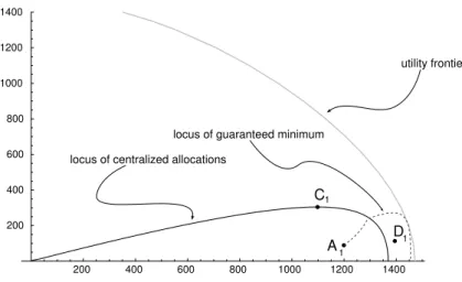
Consider next the weak solidarity case presented in figure 2, where γ = 0.005. The locus of centralized allocations looks very similar to that of the no solidarity case: it starts at the origin (when t = 0), and grows until pointC1, when the poor region’s utility is maximized. For the poor region, represented in the vertical axis, a further increase in the tax rate (and thus a higher transfer from the rich), will not be compensated by the more than proportional increase in public spending because too little resources are left for private consumption. For high tax rates,t= 0.5, the poor region’s utility falls below survival. The whole curve lies below the Pareto-efficient utility frontier.
decentral-200 400 600 800 1000 1200 1400 200 400 600 800 1000 1200 1400 D1 C1 A1 utility frontier
locus of centralized allocations
locus of guaranteed minimum
Figure 2: The utility allocations in the weak solidarity case
ized and autarchy points are no longer Pareto optimal: they lie in the inte-rior of the utility possibility set. The decentralized equilibrium,D1, Pareto dominates the autarchy equilibrium,A1. The decentralized equilibrium D1 is much closer to the efficiency frontier and Pareto dominates a good portion of the locus of centralized allocations. But it is in turn Pareto dominated by a mixture of centralized taxes complemented by local taxation.
As was to be expected, the autarchy point,A1, coincides with the locus of the guaranteed minimum system when the tax rate ist= 0. As the tax rate grows, we observe that both utilities increase. Eventually, the poor region reaches the point at which the centrally financed public expenditure is enough and th optimal local public expenditure is zero. From that point on, the nonnegativity constraint forg2in expression (37) is binding and only the rich region uses local taxation for increasing public expenditure. The transition to the new region can be seen in the graph as a kink in the curve. There are many points in this locus (i.e., many central tax rates t) that lead to allocations that Pareto dominate the decentralized allocationD1. In brief, by comparing figures 2 and 1, we see that when solidarity is positive, but small, the decentralized system is no longer Pareto optimal but still it seems superior to the decentralized system.
3.4 The strong solidarity case
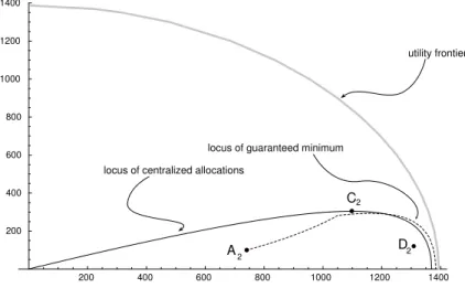
Consider next the case of strong solidarity, γ = 0.05, which is represented in figure 3.
200 400 600 800 1000 1200 1400 200 400 600 800 1000 1200 1400 D2 C2 A2 utility frontier
locus of centralized allocations
locus of guaranteed minimum
Figure 3: The utility allocations in the strong solidarity case
Again, all the outcomes are inefficient, but the centralized locus gets closer to the efficiency frontier. The decentralized equilibrium, D2, still Pareto dominates the autarchy equilibrium. And finally, there is a signifi-cant range of taxes for which the centralized solution Pareto dominates the decentralized equilibrium, D2. The centralized system is superior to the decentralized one.
As before, the mixed model of centralized taxes complemented by local taxation performs very well. Most of the second best efficient part of the locus of centralized allocations is Pareto dominated by a solution obtained from the combination of central and local taxes.
4 Some empirical facts
Our theoretical analysis and simulations predict that, in countries with a stronger taste for solidarity, it may be more efficient for the central govern-ment to control the provision of local public goods and services. This result implies a negative relationship between the strength of solidarity prefer-ences and the degree of fiscal decentralization. In this section, we present cross-country empirical evidence consistent with this prediction.
Relying on data from the International Monetary Fund’s Government
Finance Statistics 2002, we calculate measures of decentralization and
soli-darity for each of 14 countries. Our measure of the degree of fiscal decentral-ization is regional and local own-source revenues as a share of total (local,
regional and central) own-source revenues. Although ideally the denomina-tor should be total consolidated revenues, we could not find this measure for most countries, and therefore we have chosen to miss some external-source revenues by using own-external-source revenues, rather than double count inter-governmental transfers by using unconsolidated revenues.
Our measure of the taste for solidarity is total (all levels of government) expenditures on social and welfare programs as a share ofGDP. This mea-sure attempts to capture a taste for redistribution of income, which we argue is plausibly related to a taste for redistribution of public expenditure. It would be better to have a measure of a taste for redistribution among regions. However, regional data are not available from the IMF, and, im-portantly, a measure of variance of spending at the regional level could be reflective of either a taste for solidarity or a taste for decentralization.
Table 1 displays our measures of a taste for solidarity and the degree of decentralization for 14 countries. The country selection is based solely on data availability for central, regional and local governments in 2000. We have used accrual basis data when available, although for some countries only cash-basis data are available (see the notes to the table for further details concerning the data). We present the countries in increasing order in their measure of solidarity, so that the relation between the two variables is easier to see. The two variables have a negative correlation equal to−.453.
Table 1: Solidarity and decentralization
Country Solidarity Decentralization
United States (US) 0,080 0,411
Russia (RU) 0,081 0,349 Argentina (AR) 0,090 0,403 Slovak Republic (SR) 0,116 0,050 Canada (CA) 0,129 0,523 Spain (SP) 0,135 0,189 Czech Republic (CZ) 0,138 0,161 United Kingdom (UK) 0,160 0,085
Norway (NW) 0,174 0,208 Italy (IT) 0,177 0,176 Slovenia (SL) 0,184 0,087 Croatia (CR) 0,191 0,106 France (FR) 0,206 0,125 Germany (GE) 0,225 0,345
Notes for the Table
Solidarity • All data for year 2000, except UK - 2001 and
Norway - 1999.
• Accrual basis data, except US, Slovenia, Slovak
Re-public, Russia, Czech ReRe-public, Croatia, Canada, Ar-gentina, Norway that are in cash basis Solidarity is equal to the sum of social protection at the central, regional and local level as a percentage of GDP.
• For UK, Slovak Republic and Italy solidarity is equal
to social protection at general government level as a share of GDP.
Decentralization • All data for year 2000 except Norway
-1999.
• Accrual basis data, except United States, Slovenia,
Slovak Republic, Russia, Czech Republic, Croatia, Canada, Argentina, Norway that are in cash basis data.
• Decentralization is calculated as own resources (total
revenue - grants) at the regional and local level as a share of total own resources (central, regional and local governments).
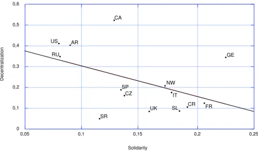
Figure 4 shows a scatter plot with solidarity on the horizontal axis and decentralization on the vertical axis, with the predictive regression line im-posed over the plot.
0 0,1 0,2 0,3 0,4 0,5 0,6 0,05 0,1 0,15 0,2 0,25 Solidarity Decentralization RU US SP CZ NW SL FR GE AR CA SR UK IT CR
Figure 4: Solidarity and decentralization for all the sample
The results of the estimated regression are presented in the first column of Table 2. We obtain a negative coefficient as predicted, however, it is statistically insignificant.
Table 2: Regression Results
All sample Excluding Germany
constant 0,445 0,546
(-0.127) (-0.120) solidarity -1,445 -2,272
(-0.820) (-0.808)
R2 0,206 0,418
Notes for the Table
Decentralization as a dependent variable. Standard errors in parentheses.
The strong leverage of the German observation leads us to consider the possibility that there may be measurement error in the decentralization vari-able, which would have a strong influence on the estimated regression. It
is in fact the case that our measure of decentralization has an upward bias for countries where regions have important ceded taxes, but have little leg-islative autonomy over them. In fact, the tax-sharing model established in Germany attributes to the L¨ander large amounts of own resources, as they administer their own taxes, but, in fact, the L¨ander have little autonomy to set tax rates, deductions and other aspects of the tax system needed to have true tax authority. Legislation regarding tax base and rates is the domain of the federal government (see Rodden, 2003).
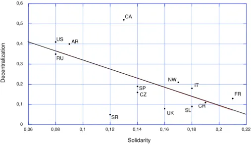
Thus, we have reason to believe that there is measurement error in our decentralization variable for Germany. We present results in Figure 4 and in column 2 of Table 2 with Germany removed from the sample.
RU US SP CZ NW SL FR AR CA SR UK IT CR 0 0,1 0,2 0,3 0,4 0,5 0,6 0,06 0,08 0,1 0,12 0,14 0,16 0,18 0,2 0,22 Decentralization Solidarity
Figure 5: Solidarity and decentralization excluding Germany
The fit improves considerably, with an important increase in the value forR2, and a slope coefficient that is negative and highly significant. Graph-ically, we also observe that the predictive regression line better describes the remaining country observations.
Given the small sample and admittedly questionable data, we are en-couraged to find the predicted negative relationship between our measure of taste for solidarity and degree of decentralization.
5 Conclusion
Many public goods and services are provided at different levels of govern-ments in different countries. An important subset of these goods and ser-vices are publicly provided private goods and serser-vices such as education and health. For these goods and services there is no advantage from a production stand point to central provision or local provision. Because of varying needs for these goods across localities, allocative efficiency is enhanced through local provision. We show that this well-known result may be turned on its head if individuals have a preference for solidarity.
In our model, solidarity is a public good in the sense that it creates externalities that are not fully internalized by a decentralized solution. Once the public good solidarity is introduced, the standard result of allocative inefficiency of the centralized solution is confronted with the inefficiency of a decentralized solution. The relative importance of the two types of inefficiencies depends on the strength of the solidarity preferences.
To be able to quantify the importance of the two types of inefficiencies present in our model and arrive at a choice of a fiscal federal system, we carry out some simulations that differ in the assumption about the strength of the solidarity parameter. If the taste for solidarity is weak, the decentral-ized solution prevails as a dominant solution, as it is closer to the efficiency frontier and is not Pareto dominated by any centralized solution. For a cer-tain range of parameters, though, a mixed model that combines a minimum centrally financed level of public good with a decentralized solution, Pareto dominates the decentralized solution. If solidarity preferences are strong, the decentralized solution is Pareto dominated by several solutions of both the centralized and the mixed systems.
Our theoretical model gives rationale to the observation that across coun-tries the degree of fiscal decentralization varies, without the need to conclude that some countries are choosing inefficient systems of decentralization. It also suggests that the stronger the solidarity preferences of individuals in a country, the less decentralized that country should be. We offer some em-pirical evidence to corroborate the negative relationship between solidarity and decentralization predicted by our model.
References:
Bird, Richard M. and Robert D. Ebel, Subsidiarity and Solidarity: The
Role of Intergovernmental Relations in Maintaining an Effective State,
McGuire, Therese J., and Teresa Garcia-Mil`a, “Solidarity and Fiscal Decen-tralization”. Proceedings - 96th Annual Conference on Taxation, Chicago,
Illinois, November 13-15, 2003. Washington DC: National Tax Association,
forthcoming 2004.
Oates, Wallace E.,Fiscal Federalism, New York, Harcourt, Brace Jovanovich, 1972.
Oates, Wallace E., “An Essay on Fiscal Federalism”, Journal of Economic
Literature, XXXVII, September 1999, pp.1120-1149.
Rodden, Jonathan, “Soft Budget Constraints and German Federalism”, in
Fiscal Decentralization and the Challenge of Hard Budget Constraints,