BOFIT Discussion Papers
20
•
2008
Pierre-Guillaume Méon
and Laurent Weill
Is corruption an efficient grease?
Bank of Finland, BOFIT
BOFIT Discussion Papers
Editor-in-Chief Iikka Korhonen
BOFIT Discussion Papers 20/2008
12.11.2008
Pierre-Guillaume Méon
and Laurent Weill:
Is corruption an efficient grease?
ISBN 978-952-462-931-7 ISSN 1456-5889
(online)
This paper can be downloaded without charge from http://www.bof.fi/bofit
or from the Social Science Research Network electronic library at http://ssrn.com/abstract_id=1304596.
Suomen Pankki Helsinki 2008
Contents
Abstract ... 3
Tiivistelmä ... 4
1 Introduction ... 5
2 Two testable hypotheses ... 7
2.1 The grease the wheels hypothesis ... 7
2.2 The sand the wheels hypothesis ... 9
3 Methodology ... 11
3.1 Measuring efficiency ... 11
3.2 Testing our competing hypotheses ... 13
4 Data ... 14
4.1 Corruption data ... 14
4.2 Governance data ... 16
4.3 Macroeconomic data and control variables ... 17
5 Results ... 19 5.1 Findings ... 19 5.2 A quantitative assessment ... 28 5.3 Robustness checks ... 29 6 Concluding remarks... 31 Appendix ... 33
A1 Countries in the sample ... 33
A2 Robustness checks ... 34
All opinions expressed are those of the authors and do not necessarily reflect the views of the Bank of Finland.
Pierre-Guillaume Méon
1and Laurent Weill
2Is corruption an efficient grease?
Abstract
This paper tests whether corruption may act as an efficient grease for the wheels of an oth-erwise deficient institutional framework. We analyze the interaction between aggregate efficiency, corruption, and other dimensions of governance for a panel of 54 developed and developing countries. Using three measures of corruption and five measures of other as-pects of governance, we observe that corruption is consistently detrimental in countries where institutions are effective, but that it may be positively associated with efficiency in countries where institutions are ineffective. We thus find evidence of the grease the wheels hypothesis.
Keywords: governance, corruption, income, aggregate productivity, efficiency. JEL Classification: C33, K4, O43, O47.
1
Université Libre de Bruxelles (ULB), DULBEA, CP-140, avenue F.D. Roosevelt 50, 1050 Bruxelles, Belgium. (phone: +32 2 650 66 48, fax: +32 2 650 38 25, e-mail: [email protected])
2
Université Robert Schuman, Institut d’Etudes Politiques, 47 avenue de la Forêt Noire, 67082 Strasbourg Cedex, France. (phone: +33 3 88 41 77 54, fax: +33 3 88 41 77 78, e-mail: [email protected])
Pierre-Guillaume Méon
and Laurent Weill
Is corruption an efficient grease?
Tiivistelmä
Tässä keskustelualoitteessa testataan, tehostaako korruptio talouden toimintaa ympäristös-sä, jossa instituutiot toimivat huonosti. Työssä tutkitaan tehokkuuden, korruption ja julki-sen hallinnon toiminnan välisiä yhteyksiä 54 maata kattavassa paneelissa, jossa on mukana sekä kehittyneitä että kehittyviä talouksia. Korruptiota mitataan kolmella eri mittarilla, ja julkisen hallinnon toiminnan tehokkuutta kuvaa viisi eri mittaria. Tulosten mukaan korrup-tio on aina haitallista, jos julkinen sektori toimii tehokkaasti, mutta korrupkorrup-tio voi tehostaa talouden toimintaa, jos julkisen sektorin instituutiot toimivat huonosti.
1
Introduction
A handful of economists have challenged the widely held notion that corruption is effi-cient.3 Leys (1965) goes so far as to wonder why people have a “problem about corrup-tion.” Aidt’s (2003) survey finds several theoretical justifications for this provocative claim. The leading argument that corruption may confer beneficial effects is known as the “grease the wheels” hypothesis proposed by Leff (1964), Leys (1965) and Hunting-ton (1968). It states that corruption may be beneficial in a second-best world by alleviating the distortions caused by ill-functioning institutions. Specifically, the grease the wheels argument postulates that an inefficient bureaucracy constitutes a major impediment to eco-nomic activity that some “speed” or “grease” money may help circumvent. Lui (1985) of-fers a formal illustration of this argument, showing that corruption can efficiently reduce the time cost of queues. Essentially, the grease the wheels hypothesis says that graft can may as a trouble-saving device in a second-best world, thereby raising economic efficien-cy.
The idea that corruption may sometimes be efficient is anathema in most policy cir-cles. International organizations such as the IMF and the OECD treat corruption as a major hindrance to economic development. Indeed, the drive to stamp out corruption has led to a range of international initiatives, including the UN Convention against Corruption, adopted in 2003, and the OECD’s “Convention on combating bribery of foreign public officials in international business transactions,” implemented in April 1999.
The view that corruption is always undesirable seems to originate in a recent strand of empirical literature quantifying the consequences of corruption. This area of study was pioneered by Mauro (1995), who observed a significant negative relationship between cor-ruption and investment that extended to growth. Mo (2001) subsequently confirmed Mauro’s results and others extended them to macroeconomic variables such as foreign di-rect investment (Wei, 2000) and productivity (Lambsdorff, 2003).
Strictly speaking though, this evidence does not allow to reject the grease the wheels hypothesis but may in fact be consistent with it. Indeed, the hypothesis simply im-plies that corruption is beneficial in countries with deficiencies in governance, but remains detrimental elsewhere. Therefore, an observation that corruption on average is associated with more disappointing economic outcomes does not prevent the correlation from being 3 Corruption is understood here in the traditional sense as misuse of public office for private benefit.
positive in those countries where governance is mediocre. The average result may be driven by the negative correlation between corruption and economic performance in the subset of countries where institutional frameworks are effective, while the correlation may be positive elsewhere.
To our knowledge, specific attempts to test the grease the wheels hypothesis remain scarce. Mauro (1995) rejected it on the grounds that he observed no significant difference in the relationship of corruption and the investment ratio between high red-tape and low red-tape countries. Ades and di Tella (1997) also rejected the hypothesis in their work. Kaufmann and Wei (1999), using firm-level data, observed that the multinationals that paid more bribes also tended to spend more time negotiating with foreign countries’ officials – a fact hard to reconcile with the grease the wheels hypothesis. Méon and Sekkat (2005), studying the hypothesis from a macroeconomic perspective, observe that corruption is gen-erally detrimental to investment and growth, especially in countries with otherwise defec-tive institutional frameworks. This evidence appears to support a converse “sand the wheels” effect of corruption.
Notably, the above-mentioned contributions focus on factor accumulation or en-dowments rather than productivity, which is the main determinant of cross-country differ-ences in economic performance. Yet, as the recent survey of Caselli (2005) points out, the evidence that cross-country differences in economic performance are the result of differ-ences in productivity is overwhelming. Consequently, testing the economic significance of corruption and the grease the wheels hypothesis requires a focus on productivity and in-quiry as to whether corruption helps countries with faulty institutions take advantage of their factor endowments. This is precisely the aim of the present paper.
Following Moroney and Lovell (1997), we apply efficiency frontiers to aggregate production functions. This approach provides a synthetic measure of the gap between the observed and optimal production of countries. The interrelationship of corruption, effi-ciency, and the quality of the institutional framework is then investigated to test the grease the wheels hypothesis by assessing the interaction between corruption and a wide range of indicators of the quality of governance for a panel of countries. Our results are consistent with the grease the wheels hypothesis.
The remainder of this paper is organized as follows. The next section briefly de-scribes the grease the wheels and sand the wheels hypotheses. Section 3 outlines our
method. Our data set is presented in section 4. We give our empirical results in section 5 and conclude in section 6.
2
Two testable hypotheses
The grease the wheels hypothesis is rooted in scholarly efforts to qualify the conclusions of the “moralistic view” of corruption.4 Some researchers stress corruption may have its own merits in fostering development, and therefore should not be judged solely on moral grounds. This line of reasoning often rests on considerations that emphasize the accommo-dative properties of graft in the presence of other imperfections in a political system. Of course, one can also readily imagine mechanisms that might make corruption more costly for deficient institutions. These mechanisms form the core of the sand the wheels hypothe-sis.
Both hypotheses distinguish between corruption and other institutional deficiencies. Leff (1964) differentiates corruption as such from bureaucratic inefficiency (inability to attain set goals). A survey of the two hypotheses is provided by Méon and Sekkat (2005). To save space here, we offer the survey’s descriptions of how the impact of corruption on efficiency may depend on the quality of the institutional framework. Our aim at this point is merely to identify a valid strategy for testing the grease the wheels and the sand the wheels hypotheses against each other.
2.1
The grease the wheels hypothesis
Unsurprisingly, bureaucratic inefficiency is recognized as the most prominent inefficiency corruption can grease,5 and particularly bureaucratic slowness. Leys (1965), therefore, looks at bribes that give bureaucrats incentive to speed up permitting of new firms in an otherwise sluggish administration. The same type of corruption is subsequently examined by Lui (1985), who shows in a formal model that corruption can efficiently reduce time spent in queues. Another problem arguably remedied by corruption may be poor quality of 4 The expression “moralistic approach” is used by both Leys (1965) and Nye (1967). Those who opposed that
view were later deemed “functionalists” or “revisionists” by their adversaries. On a general plane, they seemed to be motivated by a concern that the moral implications of corruption may bias the understanding of its economic consequences and a concern that the Western concept of graft may be ill-suited to the context of developing countries.
5 As Huntington (1968, p. 386) puts it: “In terms of economic growth, the only thing worse than a society
civil servants in a low-paid bureaucracy. Leys (1965) and Bailey (1966), for example, note that corruption perks may attract competent civil servants to a sector with otherwise low prevailing wages.
Leff (1964) and Bailey (1966) make the case that graft can sometimes act as a hedge against bad public policies, particularly if the bureaucrat is biased against, say, en-trepreneurship for ideological reasons or carries a prejudice against certain minority groups.6 By impeding inefficient regulation, corruption limits its adverse effects. Of course, the causality could be more subtle. Ehrlich and Lui (1999), for example, postulate that autocratic regimes that can centrally steer administration are more likely to implement policies that are closer, if not equivalent, to first-best policies. They follow this path be-cause they want to maximize their rents and internalize the deadweight loss associated with corruption. The autocrat has an incentive to avoid impairing the productivity of the private sector that is absent in decentralized regimes, since bureaucrats are blind to the detrimental effect of bribes on productivity. Thus, corruption provides an incentive to implement better policies in autocratic regimes but not in democratic regimes. All things being equal, cor-ruption is more beneficial in countries that are less democratic.
Moreover, it has been argued that graft may, in some circumstances, improve the quality of investments. This is particularly the case, as Leff (1964) stresses, where gov-ernment spending is inefficient. If corruption is a means of tax evasion, it can reduce the revenue of public taxes and, provided bribers have efficient investment opportunities, im-prove the overall efficiency of investment. More generally, one may contend that corrup-tion is an efficient way of selecting investment projects if such investments depend on gaining a license. Bailey (1966), for instance, claims that this may be true if the ability to offer a bribe is correlated with talent. More specifically, one may argue that awarding a license through corrupt methods is very similar to a competitive auction. Leff (1964) con-tends that favors are more likely to be allocated to the most generous bribers, which also assures they are the most efficient. Beck and Maher (1986) and Lien (1986) formally dem-onstrate that corruption replicates the outcome of a competitive auction aimed at attributing a government procurement contract as the ranking of bribes replicates the ranking of firms by efficiency.
6 Nye (1967) reports corruption was instrumental in making central planning more effective in the Soviet
Union. He also argues corruption helped increase the influence of Asian minority entrepreneurs in East Afri-ca beyond what politiAfri-cal conditions would have allowed.
All the above-mentioned arguments presume that corruption can contribute posi-tively to the productivity of the factors of production with which a country is endowed. It compensates for the consequences of a defective institutional framework, resulting in an inefficient administration, diminished rule of law, or political violence. Despite these bene-fits, of course, corruption may also impose additional costs in a weak institutional envi-ronment. The existence of such costs provides a rationale for the sand the wheels hypothe-sis.
2.2
The sand the wheels hypothesis
The sand the wheels hypothesis emphasizes that some of costs of corruption may become manifest or magnified in a weak institutional context.
For instance, the claim that corruption speeds up an otherwise sluggish bureaucracy is inconsistent. Myrdal (1968) points out that a corrupt civil servant can also have incen-tives to cause delays where there is the opportunity to extract a bribe. Further, Ku-rer (1993) shows corrupt officials have incentives to create other distortions in the econ-omy to preserve illegal sources of income. These arguments are perfectly compatible with the experience of individual bribers, who benefit personally from perks. They stress, how-ever, that nothing may be gained from corruption at the aggregate level.7
Moreover, it can be argued that corruption may not be the best way to award a li-cense to the most efficient producer, because even if the analogy between corruption and a competitive auction holds true, the winner is not necessarily the most efficient. In auctions where the profitability of a license is uncertain, the winner may simply be the most opti-mistic bidder (the “winner’s curse”). Second, as Rose-Ackerman (1997) contends, the highest briber may simply be the one most willing to compromise on the quality of the goods he will produce if he gets a license. Under such circumstances, corruption reduces efficiency.
The argument that corruption may raise the quality of investment is also dubious in the case of public investment. Mauro (1998) notes that corruption diverts public spending to less efficient allocations. Overall, corruption results in a greater amount of public
in-7 Those effects can be exacerbated when the administration is made of a succession of decision centers or
civil servants. Shleifer and Vishny (1993) construct a formal model in which the cost of corruption is greater when the administration is made up of many independent agencies rather than centrally managed.
vestment in unproductive sectors, which is unlikely to improve efficiency or promote eco-nomic growth.
Corruption could also serve as a hedge against risk in politically uncertain envi-ronments as long as the corruption does not imply additional risk-taking. What distin-guishes corruption from simple transactions is illegality. Corrupt deals can create unen-forceable contracts that lead to opportunism, especially by the bribe-taking counterparty. Furthermore, the increased uncertainty from corruption may extend beyond the corruption dealing itself. Extensive corruption has been found to be associated with large shadow economies, as noted e.g. by Dreher and Schneider (2006a, b). Since transactions in the shadow economy are by definition unregulated, they are subject to greater uncertainty than official transactions.
Bardhan (1997) argues that the inherent uncertainty of corrupt agreements may ob-viate the efficiency-enhancing mechanisms described earlier and provide an incentive, as Henisz (2000) contends, to invest in less productive general (as opposed to specific) capital that can easily be reallocated. Thus, corruption may worsen the quality of investment rather than reduce the level of investment.
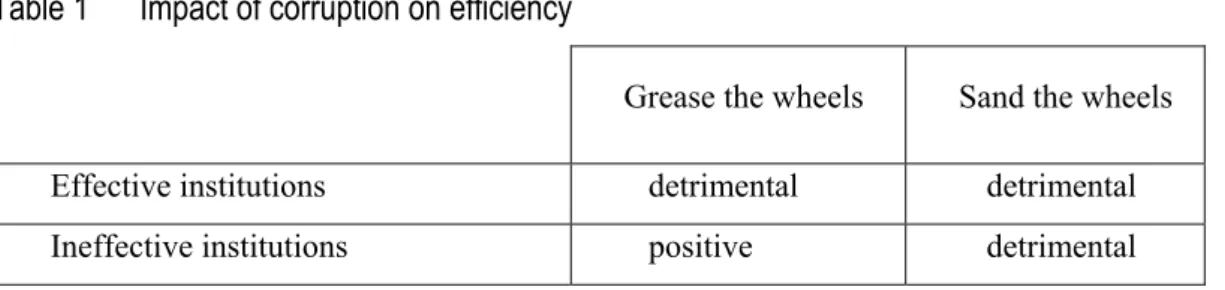
In summary, both the grease-the-wheels and sand-the-wheels hypotheses can be readily argued in the abstract. Fortunately for us, both produce the testable hypotheses summarized in Table 1:
Table 1 Impact of corruption on efficiency
Grease the wheels Sand the wheels
Effective institutions detrimental detrimental
Ineffective institutions positive detrimental
Table 1 shows both hypotheses predict that an increase in corruption will reduce efficiency in an otherwise efficient institutional context. They differ, however, in the expected impact of corruption in a deficient institutional context. The grease the wheels hypothesis predicts that corruption may help raise efficiency, while the sand the wheels hypothesis predicts that an increase in corruption will reduce efficiency even in a deficient institutional con-text.
3
Methodology
In this section, we explain how we measure aggregate efficiency and take its determinants into account.
3.1
Measuring efficiency
Our first aim is to measure aggregate efficiency in order to assess its link with corruption. With this end in mind, we assess technical efficiency, which measures how close a count-ry’s production is to what a countcount-ry’s optimal production would be for using the same bundle of inputs. We use the stochastic frontier approach developed by Aigner, Lovell and Schmidt (1977), and applied at the aggregate level notably by Adkins et al. (2002).
Macroeconomic productivity is better measured using this approach rather the more common measures of productivity for several reasons. First, this approach provides a syn-thetic measure of productivity. Unlike basic productivity measures (e.g. per capita in-come), the efficiency scores computed with the stochastic frontier approach allow us to include several input dimensions in evaluating performances. Thus, output is not only compared to the labor stock, but also the physical and human capital stocks.
Second, it provides relative measures of productivity. Here, a common production frontier is estimated, allowing the comparison of each country to the best-practice coun-tries. This gives us an efficiency score for how close a country’s actual production is to what its optimal production would be using the same bundle of inputs.
Third, whereas total factor productivity measures assess performance by the whole residual from the production frontier for each country, the stochastic frontier approach al-lows us to separate the distance to the production frontier into an inefficiency term and a random error, taking into account exogenous events.
Having assessed each country’s level of efficiency, we next determine the interrela-tionship of corruption, governance and efficiency to test the grease the wheels hypothesis against the sand the wheels hypothesis. A natural way of estimating this relationship would be to resort to a two-stage approach that involves estimating efficiency scores and regress-ing them on the relevant set of explanatory variables. Although widely used in microeco-nomic studies, this approach is inconsistent here, as it assumes in the first stage that ineffi-ciencies are independently distributed and the second-stage regression does not respect the independence assumption.
Instead, we use the one-stage approach developed by Battese and Coelli (1995), whereby the stochastic frontier model includes both a production frontier and an equation in which inefficiencies are specified as a function of explanatory variables. This approach offers greater consistency than the two-stage approach, which explains its application in studies of the determinants of technical efficiency at the aggregate level (e.g. Adkins et al., 2002).
Our stochastic frontier model thus includes two equations. The first is the specifica-tion of the producspecifica-tion frontier. We assume a constant returns-to-scale Cobb-Douglas pro-duction technology,8 which we write as
ln (Y/L)it = α0 + α1 ln (K/L)it + α2 ln (H/L)it + vit− uit , (1)
where i indexes countries and t the year of observation. (Y/L), (K/L), (H/L) are out-put per worker, capital per worker, and human capital per worker respectively. vit is a
ran-dom disturbance, which reflects luck or measurement errors. It is assumed to have a nor-mal distribution with zero mean and variance σv². uit is an inefficiency term, capturing
technical inefficiencies. It is a one-sided component with variance σu². As is common in
the literature, we assume a half-normal distribution for the inefficiency term. The second equation is the specification of inefficiencies as
uit =δ zit + Wit , (2)
where uit is country i’s inefficiency, zit is a p×1 vector of p explanatory variables, δ
is a 1×p vector of parameters to be estimated, and Wit the random variable defined by the
truncation of the normal distribution with mean zero and variance σ ² = σu² + σv².
Finally, we use the Frontier software version 4.1 developed by Coelli (1996) to per-form the maximum likelihood estimation of the stochastic frontier model.
8 When Hall and Jones (1999) estimate aggregate productivity in a related cross-country study, they find that
results obtained with a Cobb-Douglas production function are quite similar to the results obtained when the production function is not restricted to that specification. Kneller and Stevens (2003) reached similar conclu-sions when estimating aggregate efficiency frontiers.
We also adopt constant returns-to-scale. As Moroney and Lovell (1997, p. 1086) note, “At the economy-wide level, constant returns-to-scale is virtually compelling.”
3.2
Testing our competing hypotheses
The test of the grease the wheels and the sand the wheels hypotheses that we use consists in assessing how a modification of the quality of the institutional framework affects the impact of corruption on efficiency. More precisely, the relationship between the coefficient of corruption in expression 2 and the quality of governance must be assessed. Following Méon and Sekkat (2005), we do so by including an interaction term between a corruption index and a governance index in expression (2), in addition to usual explanatory variables. The estimated relationship thus reads
uit = δ0 + δ1 corrupi+δ2 corrupi× govi +δ3 govi+ δc controlit + Wit , (3a)
where uit is country i’s inefficiency, corrupi a measure of corruption, govi a measure of the
quality of its institutional framework, and controlit a vector of control variables. δ0, δ1, δ2,
and δ3 are scalars, whereas δc is a vector of coefficients.
A reformulation of expression (3) shows more clearly how it can be used to test the grease the wheels and sand the wheels hypotheses:
uit = δ0 + (δ1+ δ2 × govi) corrupi+ δ3 govi+ δc controlit + Wit . (3b)
The key parameters here are δ1 and δ2. To understand why, we first assume the sand- the-wheels hypothesis holds. In this case, corruption always has a negative impact on efficiency and that impact worsens as the institutional framework deteriorates. The coeffi-cient of corruption must therefore always be positive, but less so when the institutional framework is efficient. Accordingly, δ1 must be positive and δ2 negative. Thus, the positive impact of corruption on inefficiency is a decreasing function of the quality of the other di-mensions of governance.
Let us now assume instead that the grease the wheels hypothesis holds. In this case, corruption has a positive effect on efficiency when the quality of governance is very low. The effect becomes negative as the quality of governance rises. Thus, corruption has a negative impact on inefficiency if the index of governance is close to zero. For the coeffi-cient of corruption to be negative when govi is very small, the coefficient δ1 must be
nega-tive. However, the grease the wheels hypothesis implies that inefficiency is positively cor-related with corruption when governance is satisfactory, i.e. when govi is large. δ2 must
therefore be positive. Moreover, for the grease the wheels hypothesis to be verified, the value must be such that the overall coefficient of the corruption index (δ1+ δ2 × govi) may
be negative for low values of the governance parameter. In other words, corruption must be negatively associated with inefficiency for at least the worst governed country.
Of course, the fact that δ1 and δ2 bear the necessary signs does not ensure that the grease the wheels hypothesis, as defined in the previous section, strictly holds. Instead, the value of the coefficients and the range of the relevant governance index can be such that no country in our sample will present a negative overall coefficient of corruption. In this case, the observed coefficients simply mean that corruption is detrimental everywhere, but less so in countries with the poor governance.
This suggests we are dealing with two forms of the grease the wheels hypothesis that depend on the value of the coefficients and the range of the relevant governance index. Where the relevant governance index reach a low enough level that the overall coefficient of corruption is negative, greater corruption may reduce aggregate inefficiency in some countries. We designate this as the “strong” form of the grease the wheels hypothesis. Al-ternatively, when no country in the sample exhibits a sufficiently low institutional quality for the overall coefficient of corruption to turn positive, then the estimated coefficients only imply that corruption is less detrimental in countries plagued by a deficient institu-tional framework than in other countries. Corruption remains positively correlated with inefficiency in all countries. This is the “weak” form of the grease the wheels hypothesis.
Notably, even the strong form of the grease the wheels hypothesis never implies corruption improves efficiency in all countries, but only in those where governance is in-adequate.
4
Data
We use three sets of data: measures of corruption, measures of the quality of governance, and macroeconomic data.
4.1
Corruption data
There is a lack of consensus on how to measure “the use of public office for private gains” (see e.g. Bardhan, 1997). Basically, available measures of corruption that allow cross-country comparisons fall into three broad categories. The first set of indicators uses pools
.11
of experts to assess the level of corruption that prevails in a country. Typically, these rat-ings come from private risk-rating agencies. The Business International Corporation index, for example, was used by Mauro (1995). The second type of index is based on the results of surveys conducted on residents. These are usually carried out by international or non-governmental organizations. The index in the World Economic Forum’s Global Competi-tiveness Report, which was used by Wei (2000), falls into this category.
The third category consists of composite indices that aggregate those of the previ-ous two categories. A composite index has two large advantages. First, it allows the biases of specific indices to cancel each other out, therefore determining an average opinion of corruption. Basic indicators are often subject to bias since they are subjective by construc-tion. Second, a composite index can provide data for wider samples of countries because they aggregate several indices and thereby allow one index to fill the gaps of another.
In this study, we use two composite indices and one survey index to assess the con-sequences of corruption. Each index is used as a robustness check and for comparison with previous studies. We focus on the corruption index provided by the World Bank (WB), and complement our results with those obtained with the Corruption Perception Index (CPI) published by Transparency International and the corruption index used by Wei (2000).
The annual CPI index values are posted on Transparency International’s website. This overall index value is simply an average of other indices. It ranges from zero (most corrupt) to ten (least corrupt). For the sake of clarity, we used the opposite of this index in our computations so that an increase in the index can be directly interpreted as an increase in the level of corruption.
While the WB corruption indicator is also a composite index, it is estimated by an unobserved component model, and thus not a simple average of existing indices.9 The CPI and the WB indices also differ in the sets of basic indicators of corruption they aggre-gate.10 Thus, the two indices complement each other as they aggregate two different sets of
indicators using two different methods
The WB indicator can be found in the governance database posted on the World Bank’s website. It ranges from −2.5 to +2.5. Like the CPI index, it is built so that an in-crease of the index reflects better control over corruption. To transform it from an indicator 9 The construction of the World Bank’s index is described in Kaufmann et al. (1999a).
10 Exhaustive descriptions of the composition of each indicator are provided in Lambsdorff (1999) and
Kaufmann et al. (1999b).
11 Dreher et al. (2007) found the CPI was strongly correlated with estimates of the extent of corruption based
of probity to an indicator of corruption, we rescale it so that it increases with the level of corruption.
Wei’s index is an extension of the corruption index published in the World Eco-nomic Forum’s Global Competitiveness Report 1997. To increase the coverage of his data-set, Wei (2000) filled the gaps left by that first index with the information provided by the World Bank’s World 1997 Development Report.
Finally, in order to properly compare their estimates, all three indices were rescaled so as to range from 0 to 10.
4.2
Governance data
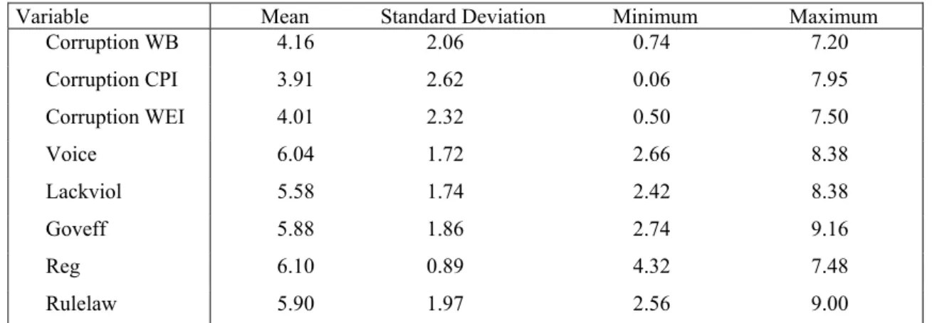
Like corruption, other facets of governance do not lend themselves easily to objective eva-luation. Quantitative indicators of governance therefore rest on subjective evaluations. To date, the largest and most comprehensive set of data assessing institutional quality is the dataset from which our second corruption measure was extracted. Kaufmann et al. (1999a, b) classify available indicators of governance into six clusters and aggregated them into as many composite indices.12 Each composite indicator represents a different dimension of governance and ranges from –2.5 to +2.5, with higher values associated with better nance. These are all rescaled to range from 0 to 10, with 10 corresponding to best gover-nance. Having explained the WB corruption index above, we simply give the definitions here of the other five indicators reported in Kaufmann et al. (1999b).
Table 2 Summary statistics on corruption and other governance variables
Variable Mean Standard Deviation Minimum Maximum
Corruption WB 4.16 2.06 0.74 7.20 Corruption CPI 3.91 2.62 0.06 7.95 Corruption WEI 4.01 2.32 0.50 7.50 Voice 6.04 1.72 2.66 8.38 Lackviol 5.58 1.74 2.42 8.38 Goveff 5.88 1.86 2.74 9.16 Reg 6.10 0.89 4.32 7.48 Rulelaw 5.90 1.97 2.56 9.00
Higher values of corruption indices indicate a greater prevalence of corruption, while other indices increase with the governance quality. Those statistics are computed for the sample of 54 countries.
12 For an example of utilization of those indices, one may either refer to the original paper of Kaufmann et
The first pair of indicators measures aspects of governance that have been the focus of a literature devoted to assessing the impact of democracy and political stability. More pre-cisely, Kaufmann et al. (1999a, b) “voice and accountability” indicator (Voice) measures “the extent to which citizens of a country are able to participate in the selection of govern-ments,” and serves as a proxy for openness of the political system. The “lack of political violence” indicator (Lackviol) provides an assessment of the political risk associated to a country, and “measures perceptions of the likelihood that the government in power will be destabilized or overthrown by possibly unconstitutional and/or violent means.”
The second pair of indicators assesses the soundness of a country’s policies and the quality of the administration in charge of implementing them. The indicator “government effectiveness” (Goveff) concerns the “perceptions of the quality of public service provi-sion, the quality of the bureaucracy, the competence of the civil servants, the independence of the civil service from political pressures, and the credibility of the government’s com-mitment to policies.” The “regulatory burden” indicator (Reg) captures “the incidence of market unfriendly policies such as price controls or inadequate bank supervision, as well as perceptions of the burden imposed by excessive regulation.”
The final indicator provided by Kaufmann et al. (1999a, b) assesses the level of spect of citizens have for their country’s legal framework. This “rule of law” indicator re-fers to “the extent to which agents have confidence in and abide by the rules of society” (Rulelaw). A chief component of this cluster is the enforceability of contracts.
4.3
Macroeconomic data and control variables
Real output per worker and labor force data are taken from the World Bank Indicators da-tabase. Real-capital-per-worker data are provided by Nehru and Dhareshwar (1994). They were complemented after 1990 by applying the perpetual inventory method on real invest-ment figures from the World Bank. Because they are measured in local currency at 1987 prices, and because our computations require comparisons of output and input levels, we convert them in US dollars using the annual average exchange rate provided by the Macro time series database of the World Bank. To smooth the impact of extreme exchange rate fluctuations, we use an average of the exchange rate computed over the period 1985-1989. Human capital is proxied by the total number of years of schooling of the working-age population over 15 years old. That dataset is taken from the Barro-Lee (2000) education dataset and can be downloaded from the Economic Growth Resources website.
Given the limited size of our sample, we restrict ourselves to three control variables commonly used in the literature. The first is openness to trade (Openness), which we proxy with the Sachs and Warner (1995) index. Although the debate on the impact of trade on growth is at least as old as economics itself, recent evidence from Edwards (1998) and oth-ers suggests openness may be positively linked to productivity.
The second control variable is the index of ethno-linguistic fractionalization (Ethno. Frac.). This index measures the probability that two individuals drawn at random from the population of a country do not speak the same language. This index is used by Mauro (1995) as well as Hall and Jones (1999). Here, we use it as a proxy for a source of long-term political unrest in a country.
Our third control variable is latitude (Latitude). While a negative correlation be-tween the distance from the equator and economic performance has been reported by nu-merous authors (e.g. Sachs, 2001), no consensual explanation to this finding exists.13
We focus on the period 1994-1997 as 1997 is the last for which a capital-per-worker ratio is available. Using the contemporaneous vintages of corruption and govern-ance indices, we gather a dataset for a sample of up to 54 countries. Descriptive statistics are provided in Table 3. The sample features both developed and developing countries.
Table 3 Summary statistics on economic and control variables
Variable Mean Standard Deviation Minimum Maximum
Y/L 13,856.84 14,844.14 317.99 43,917.22 K/L 44,392.18 50,528.82 819.42 168,891.01 H/L 10.91 4.56 2.94 18.37 Latitude 27.82 17.76 0.23 60.21 Openness 87.96 30.62 0.00 1.00 Ethno. Frac. 37.96 30.16 0.00 90.00
Y/L = output per worker; K/L = capital per worker; and H/L = human capital per worker. These statistics are computed for the sample of 54 countries.
13 Hall and Jones (1999) suggest that the history of former colonies may be linked to their location. However,
5
Results
This section presents the main results of our estimations, provides an assessment of their significance, and discusses our robustness checks.
5.1
Findings
Tables 4a to 4e display our first set of results. In each table, we study the interaction be-tween corruption and a different dimension of governance. For each of our three corruption indices, the relationship is estimated twice; first without interaction between corruption and governance, then incorporating the interaction term. The first five lines exhibit the coeffi-cients of the estimated production frontier, and the lower part of the table is devoted to the coefficients of the equation in which inefficiency is explained.14 Three year-dummies for 1994, 1995, and 1996 (Year94, Year95, and Year96, respectively) were introduced to the specification of the production function to control for possible year-specific fluctuations of the frontier.
At first glance, the estimated production frontiers are stable across estimations. Moreover, estimated coefficients are similar to those reported in the literature (e.g. Kneller and Stevens, 2003). Year-dummies never exhibit a significant coefficient, suggesting that no major shift of the frontier was observed for the years featured in our study.
In addition, all control variables are either intuitively signed or insignificant. Thus the openness index is usually correctly signed and often significant. The only exception appears with the CPI, where openness can bear a positive and significant sign, although not in all regressions, and in particular not in those that feature the interaction term between the CPI and governance. The relationship between inefficiency and latitude is less surpris-ing. As expected, the sign of its coefficient is either insignificant or negative, implying that inefficiency ceteris paribus tends to decrease as one moves away from the equator. Finally, ethnic fractionalization is more robust than latitude; it is positively and significantly asso-ciated with inefficiency in eleven estimations. Accordingly, more ethnic homogeneity ap-pears to be positively correlated with aggregate efficiency.
14 A minus sign indicates that an increase in the explanatory variable leads to less inefficiency (i.e. a rise in
With regards to the institutional and corruption variables, the general picture that emerges from Tables 4a to 4e is strikingly consistent across specifications, and regardless of the governance variable taken into account. Thus, in benchmark estimations (odd-numbered), the relevant governance indicator is negatively signed or insignificant, excep-tion for voice and accountability in the estimaexcep-tion that also features the CPI among regres-sors. Accordingly, aggregate efficiency rises with the quality of governance as measured by the World Bank indicators.
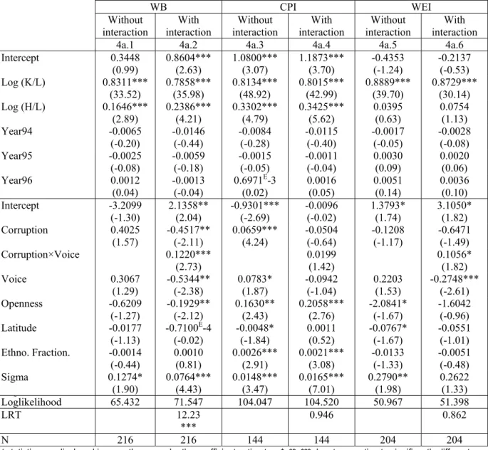
Table 4a Estimation with voice and accountability as the governance variable
WB CPI WEI
Without
interaction interaction With interaction Without interaction With interaction Without interaction With 4a.1 4a.2 4a.3 4a.4 4a.5 4a.6 Intercept 0.3448 (0.99) 0.8604*** (2.63) 1.0800*** (3.07) 1.1873*** (3.70) -0.4353 (-1.24) -0.2137 (-0.53) Log (K/L) 0.8311*** (33.52) 0.7858*** (35.98) 0.8134*** (48.92) 0.8015*** (42.99) 0.8889*** (39.70) 0.8729*** (30.14) Log (H/L) 0.1646*** (2.89) 0.2386*** (4.21) 0.3302*** (4.79) 0.3425*** (5.62) 0.0395 (0.63) 0.0754 (1.13) Year94 -0.0065 (-0.20) -0.0146 (-0.44) -0.0084 (-0.28) -0.0115 (-0.40) -0.0017 (-0.05) -0.0028 (-0.08) Year95 -0.0025 (-0.08) -0.0059(-0.18) -0.0015 (-0.05) -0.0011 (-0.04) 0.0030 (0.09) 0.0020 (0.06) Year96 0.0012 (0.04) -0.0013 (-0.04) 0.6971 E-3 (0.02) 0.0016 (0.05) 0.0051 (0.14) 0.0036 (0.10) Intercept -3.2099 (-1.30) 2.1358** (2.04) -0.9301*** (-2.69) -0.0096 (-0.02) 1.3793* (1.74) 3.1050* (1.82) Corruption 0.4025 (1.57) -0.4517** (-2.11) 0.0659*** (4.24) -0.0504 (-0.64) -0.1208 (-1.17) -0.6471 (-1.49) Corruption×Voice 0.1220*** (2.73) 0.0199 (1.42) 0.1056* (1.82) Voice 0.3067 (1.29) -0.5344** (-2.38) 0.0783* (1.87) -0.0942 (-1.04) 0.2203 (1.53) -0.2748*** (-2.61) Openness -0.6209 (-1.27) -0.1929** (-2.12) 0.1630** (2.43) 0.2058*** (2.76) -2.0841* (-1.67) -1.6042 (-0.96) Latitude -0.0177 (-1.13) -0.7100E-4 (-0.02) -0.0048* (-1.84) 0.0011 (0.52) -0.0767* (-1.67) -0.0551 (-1.01) Ethno. Fraction. -0.0014 (-0.44) 0.0010 (0.81) 0.0026*** (2.91) 0.0021*** (3.08) -0.0133 (-1.33) -0.0051 (-0.48) Sigma 0.1274* (1.90) 0.0764*** (4.43) 0.0148*** (3.47) 0.0165*** (7.01) 0.2790** (1.98) 0.2622 (1.33) Loglikelihood 65.432 71.547 104.047 104.520 50.967 51.398 LRT 12.23 *** 0.946 0.862 N 216 216 144 144 204 204
t-statistics are displayed in parentheses under the coefficient estimates. *, **, *** denote an estimate significantly different from zero at the 10%, 5% or 1% level.
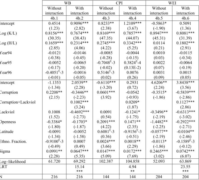
Table 4b Estimation with lack of political violence as the governance variable
WB CPI WEI
Without
interaction interaction With interaction Without interaction With interaction Without interaction With 4b.1 4b.2 4b.3 4b.4 4b.5 4b.6 Intercept 0.4514 (1.23) 0.9096*** (2.82) 0.8233** (2.38) 1.2109*** (3.67) -0.5863* (-1.90) 0.5091 (1.36) Log (K/L) 0.8156*** (30.35) 0.7674*** (38.43) 0.8169*** (47.35) 0.7857*** (44.07) 0.8947*** (45.31) 0.8081*** (31.39) Log (H/L) 0.1659*** (2.85) 0.2314*** (4.06) 0.2745*** (4.22) 0.3342*** (5.25) 0.0114 (0.21) 0.1802*** (2.91) Year94 -0.0121 (-0.38) -0.0146 (-0.45) -0.0085 (-0.28) -0.0044 (-0.15) 0.0010 (0.03) -0.0115 (-0.34) Year95 -0.0052 (-0.17) -0.0065 (-0.20) -0.7048E-3 (-0.02) 0.3824E-4 (0.13E-2) 0.0022 (0.07) -0.0064 (-0.19) Year96 -0.4051E-3 (-0.01) -0.0016 (-0.05) 0.5146 E-3 (0.02) 0.0076 (0.26) 0.0031 (0.09) 0.0015 (0.05) Intercept -1.1353 (-1.34) 2.0539** (2.28) -0.6110*** (-3.20) 0.2931 (0.72) 4.6206** (2.24) 3.8438*** (3.56) Corruption 0.2208** (2.15) -0.3446** (-2.23) 0.0601*** (3.92) -0.0542 (-0.93) -0.3515* (-1.86) -0.5839*** (-2.86) Corruption×Lackviol 0.1002*** (3.24) 0.0209* (1.87) 0.1127*** (2.86) Lackviol 0.1008 (1.52) -0.4692*** (-2.73) 0.0091 (0.54) -0.1241* (-1.75) -0.3496** (-2.19) -0.6313*** (-3.02) Openness -0.3384* (-1.80) -0.1703* (-1.87) 0.2091*** (4.22) 0.1471** (2.35) -1.4482** (-2.25) -0.2922*** (-2.71) Latitude -0.0091 (-1.34) -0.0052 (-1.58) 0.6081 E-3 (0.36) -0.9156 E-3 (-0.51) -0.0577** (-2.19) -0.0104** (-2.46) Ethno. Fraction. -0.9100E-3 (-0.49) 0.0007 (0.49) 0.0024*** (3.66) 0.0018** (2.29) -0.0113* (-1.86) -0.1589 E-3 (-0.12) Sigma 0.0991** (2.28) 0.0647*** (5.35) 0.0147*** (5.09) 0.0172*** (7.69) 0.2465*** (3.02) 0.0742*** (6.07) Log−likelihood 61.720 69.292 102.387 104.858 52.093 63.869 LRT 15.14 *** 4.94 ** 23.55 *** N 216 216 144 144 204 204
t-statistics are displayed in parentheses under the coefficient estimates. *, **, *** denote an estimate significantly different from zero at the 10%, 5% or 1% level.
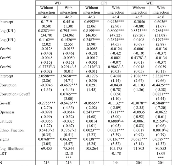
Table 4c Estimation with government efficiency as the governance variable
WB CPI WEI
Without
interaction interaction With interaction Without interaction With interaction Without interaction With
4c.1 4c.2 4c.3 4c.4 4c.5 4c.6 Intercept 0.1719 (0.50) 0.4516 (1.30) 0.6992** (2.06) 0.9436*** (2.90) -0.3056 (-0.80) 0.6036* (1.67) Log (K/L) 0.8283*** (34.70) 0.7951*** (34.96) 0.8199*** (46.05) 0.8000*** (47.22) 0.8573*** (29.20) 0.7864*** (31.08) Log (H/L) 0.1162** (2.02) 0.1526** (2.55) 0.2487*** (3.90) 0.2874*** (4.65) 0.0408 (0.68) 0.1797*** (2.88) Year94 -0.0128 (-0.40) -0.0155 (-0.46) -0.0085 (-0.28) -0.0124 (-0.42) -0.0061 (-0.19) -0.0136 (-0.37) Year95 -0.0048 (-0.15) -0.0050 (-0.15) -0.0017 (-0.05) -0.0021 (-0.07) 0.4378E-3 (0.01) -0.0134 (-0.37) Year96 -0.7773E-3 (-0.02) 0.2914 E-3 (0.01) -0.2176 E-3 (-0.01) 0.9863 E-3 (0.03) 0.0018 (0.05) 0.0039 (0.11) Intercept 2.0598*** (2.86) 3.9650*** (4.71) -0.1276 (-0.50) 0.4688 (1.14) 2.1086*** (2.67) 3.3328*** (9.66) Corruption -0.0946 (-1.35) -0.4692*** (-3.43) 0.0291 (1.45) -0.0430 (-0.78) -0.1103 (-1.36) -0.4425*** (-5.38) Corruption×Goveff 0.0765*** (3.00) 0.0090 (1.10) 0.0821*** (4.44) Goveff -0.2755*** (-2.70) -0.6426*** (-4.35) -0.0565** (-2.02) -0.1132** (-2.09) -0.3078** (-2.55) -0.5848*** (-7.20) Openness -0.0991 (-0.99) -0.0614 (-0.52) 0.2473*** (4.68) 0.1711*** (3.00) -0.0935 (-0.92) -0.0622 (-0.61) Latitude -0.0056 (-1.27) -0.0025 (-0.67) 0.0014 (1.01) 0.6880 E-4 (0.05) -0.0061 (-0.83) 0.2159 E-3 (0.06) Ethno. Fraction. 0.5410E-3 (0.35) 0.7762 E-3 (0.51) 0.0023*** (3.23) 0.0021*** (3.39) 0.0017 (0.97) 0.0010 E-2 (0.79) Sigma 0.0768*** (3.05) 0.0632*** (5.57) 0.0138*** (5.24) 0.0136*** (5.52) 0.0685*** (3.14) 0.0589*** (4.37) Log−likelihood 69.453 75.544 105.264 105.175 71.803 80.853 LRT 12.18 *** -0.178 18.09 *** N 216 216 144 144 204 204
t-statistics are displayed in parentheses under the coefficient estimates. *, **, *** denote an estimate significantly different from zero at the 10%, 5% or 1% level.
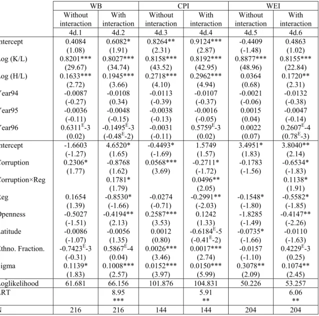
Table 4d Estimation with quality of the regulatory framework as the governance variable
WB CPI WEI
Without
interaction interaction With interaction Without interaction With interaction Without interaction With 4d.1 4d.2 4d.3 4d.4 4d.5 4d.6 Intercept 0.4084 (1.08) 0.6082* (1.91) 0.8264** (2.31) 0.9124*** (2.87) -0.4409 (-1.48) 0.4863 (1.02) Log (K/L) 0.8201*** (29.67) 0.8027*** (34.74) 0.8158*** (43.52) 0.8192*** (42.95) 0.8877*** (48.96) 0.8155*** (22.84) Log (H/L) 0.1633*** (2.72) 0.1945*** (3.66) 0.2718*** (4.10) 0.2962*** (4.94) 0.0364 (0.68) 0.1720** (2.31) Year94 -0.0087 (-0.27) -0.0108 (0.34) -0.0113 (-0.39) -0.0107 (-0.37) -0.0021 (-0.06) -0.0132 (-0.38) Year95 -0.0036 (-0.11) -0.0048 (-0.15) -0.0038 (-0.13) -0.0016 (-0.05) 0.0015 (0.04) -0.0047 (-0.14) Year96 0.6311E-3 (0.02) -0.1495 E-3 (-0.48E-2) -0.0031 (-0.11) 0.5759 E-3 (0.02) 0.0022 (0.07) 0.2607 E-4 (0.78E-3) Intercept -1.6603 (-1.27) 4.6520* (1.65) -0.4493* (-1.69) 1.5749 (1.57) 3.4951* (1.83) 3.8040** (2.14) Corruption 0.2306* (1.77) -0.8768 (1.62) 0.0568*** (3.69) -0.2711* (-1.72) -0.1783 (-1.56) -0.6534* (-1.83) Corruption×Reg 0.1781* (1.79) 0.0496** (2.05) 0.1138* (1.91) Reg 0.1654 (1.39) -0.8530* (-1.66) -0.0274 (-0.71) -0.2991** (-2.03) -0.1548* (-1.80) -0.5582* (-1.85) Openness -0.5027 (-1.51) -0.4194** (2.13) 0.2587*** (3.53) 0.1242 (1.33) -1.8285 (-1.49) -0.4147** (-2.26) Latitude -0.0086 (-1.07) -0.0056 (1.35) 0.0012 (0.80) -0.6184E-5 (-0.41E-2) -0.0735* (-1.66) -0.0110 (-1.63) Ethno. Fraction. -0.7423E-3 (-0.31) 0.5867 E-4 (0.04) 0.0026*** (3.46) 0.0017*** (2.74) -0.0157 (-1.10) 0.4229 E-3 (0.25) Sigma 0.1139* (1.83) 0.1008*** (2.57) 0.0152*** (3.97) 0.0150*** (5.99) 0.3078** (2.09) 0.1074** (2.45) Loglikelihood 61.681 66.156 101.876 104.831 50.226 53.257 LRT 8.95 *** 5.91 ** 6.06 ** N 216 216 144 144 204 204
t-statistics are displayed in parentheses under the coefficient estimates. *, **, *** denote an estimate significantly different from zero at the 10%, 5% or 1% level.
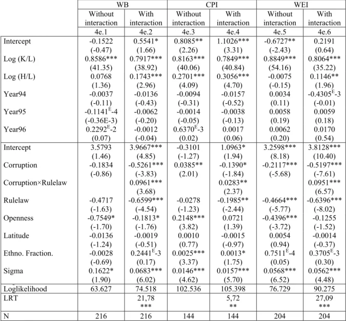
Table 4e Estimation with the rule of law as the governance variable
WB CPI WEI
Without
interaction interaction With interaction Without interaction With interaction Without interaction With
4e.1 4e.2 4e.3 4e.4 4e.5 4e.6
Intercept -0.1522 (-0.47) 0.5541* (1.66) 0.8085** (2.26) 1.1026*** (3.31) -0.6727** (-2.43) 0.2191 (0.64) Log (K/L) 0.8586*** (41.35) 0.7917*** (38.92) 0.8163*** (40.06) 0.7849*** (40.84) 0.8849*** (54.16) 0.8064*** (35.22) Log (H/L) 0.0768 (1.36) 0.1743*** (2.96) 0.2701*** (4.09) 0.3056*** (4.70) -0.0075 (-0.15) 0.1146** (1.96) Year94 -0.0037 (-0.11) -0.0136 (-0.43) -0.0094 (-0.31) -0.0157 (-0.52) 0.0034 (0.11) -0.4305E-3 (-0.01) Year95 -0.1141E-4 (-0.36E-3) -0.0062 (-0.20) -0.0014 (-0.05) -0.0038 (-0.13) 0.0058 (0.19) 0.0059 (0.18) Year96 0.2292E-2 (0.07) -0.0012 (-0.04) 0.6370E-3 (0.02) 0.0017 (0.06) 0.0062 (0.20) 0.0170 (0.54) Intercept 3.5793 (1.46) 3.9667*** (4.85) -0.3101 (-1.27) 1.0963* (1.94) 3.2598*** (8.18) 3.8128*** (10.40) Corruption -0.1834 (-0.86) -0.5261*** (-3.83) 0.0385** (2.01) -0.1390* (-1.84) -0.2117*** (-5.68) -0.5197***(-7.61) Corruption×Rulelaw 0.0961*** (3.68) 0.0283** (2.37) 0.0951*** (6.57) Rulelaw -0.4717 (-1.63) -0.6599*** (-4.54) -0.0278 (-1.23) -0.1985** (-2.44) -0.4664*** (-5.77) -0.6396***(-8.02) Openness -0.7549* (-1.70) -0.1813* (-1.76) 0.2148*** (3.82) 0.0721 (1.39) -0.4396*** (-3.72) -0.1255 (-1.52) Latitude -0.0136 (-1.24) -0.0019 (-0.51) 0.0010 (0.77) -0.0015 (-0.97) 0.0054 (0.94) -0.0014 (-0.37) Ethno. Fraction. -0.0028 (-0.69) 0.2441 E-3 (0.17) 0.0025*** (3.37) 0.0013* (1.75) 0.7511 E-4 (0.05) 0.3705 E-3 (0.30) Sigma 0.1622* (1.90) 0.0683*** (6.02) 0.0146*** (4.62) 0.0157*** (5.70) 0.0568*** (6.52) 0.0562*** (4.48) Loglikelihood 63.627 74.518 102.536 105.398 76.729 90.275 LRT 21,78 *** 5,72 ** 27,09 *** N 216 216 144 144 204 204
t-statistics are displayed in parentheses under the coefficient estimates. *, **, *** denote an estimate significantly different from zero at the 10%, 5% or 1% level.
In the same benchmark estimations, corruption indices lead to the same qualitative results. The coefficient that affects corruption is positive in six estimations out of fifteen, insignifi-cant in seven, and negative in only two estimations. If anything, this finding means that greater corruption is associated on average with greater inefficiency in the sample of our study. Again, these results are in line with previous results on the impact of corruption on growth (e.g. Mauro, 1995), or productivity growth (e.g. Olson et al., 2000).
However, the most striking result, which is central to the question that is raised in the present paper, materializes in even-numbered estimations, i.e. when the interaction term between corruption and other facets of governance is added to the set of explanatory
variables. The coefficients that were significant in odd-numbered estimations remain sig-nificant after including the interaction term. The only exception is the voice and account-ability index in estimation 4a.4. In some estimations, coefficients that were not significant become significant. This is particularly true in the case of governance indices that are al-most always significantly negative in these estimations, even though they were often insig-nificant in previous estimations. Moreover, log-likelihood most of the time substantially increases with the inclusion of the interaction term, and even-numbered estimations pass the log-likelihood ratio test against odd-numbered ones. The last two findings argue against the pooling of countries regardless of the quality of the institutional framework.
The truly remarkable feature of the even-numbered estimations appears when one looks at the coefficients of corruption and of the interaction term. In these estimations, cor-ruption exhibits either a negative or insignificant coefficient, and the interaction term is either positive or insignificant. In terms of our specification, these results mean that δ1 is generally negative, while δ2 is positive. Thus, this evidence supports the grease the wheels hypothesis.
A finding that δ1 is negative and δ2 positive can be consistent with both the strong and the weak forms of the grease the wheels hypothesis. As indicated by expression (3b) discriminating between the two versions of the grease the wheels hypothesis requires de-termining whether parameters δ1 and δ2 are such that the overall impact of corruption on inefficiency may be negative for some low values of the relevant governance index. In or-der to determine whether the displayed estimations are consistent with the strong version of the grease the wheels hypothesis, we look at each estimation and examine jointly the estimated δ1 and δ2, and the range of the relevant governance index in the sample.
With these remarks in mind, one can classify our featured estimations in three cate-gories. The first category consists of the estimations that show no sign of any relationship between corruption and efficiency. These are the estimations where neither δ1 nor δ2 is sig-nificant. Estimations 4a.4. and 4c.4 fall into this category.
The other two categories are those consistent with either form of the grease the wheels hypothesis.15 These require closer scrutiny. The weak form of the hypothesis ap-pears in estimations 4a.6, 4b.4, and 4d.2; δ2 is significantly positive, but δ1 is not
signifi-15 There is no estimation where corruption remains positively and significantly correlated with inefficiency
after the introduction of the interaction term. In other words, we find no instance of the sand the wheels hy-pothesis.
cantly different from zero. As governance indices are always positive, these estimations imply that corruption is positively associated with inefficiency in all countries, but more so in countries where governance is satisfactory. This is precisely what the weak form of the grease the wheels hypothesis predicts.
The last category comprises all the estimations that show evidence of the strong form of the grease the wheels hypothesis. The δ1 and δ2 coefficients of those estimations are such that the overall coefficient of corruption can be negative, at least for the country that exhibits the lowest value of the governance index. To illustrate this phenomenon, let us for instance focus on estimation 4c.2, which estimates the interaction between corrup-tion, as measured by the World Bank index, and government effectiveness. According to this estimation, δ1 ≅ −0.4692 and δ2 ≅ 0.0765. In addition, the country that fares worst in terms of government effectiveness (Zimbabwe) scores 2.74 on the government effective-ness index. Consequently, the total coefficient of corruption for this country is equal to (−0.4692 + 0.0765 × 2.74) ≅ −0.2596. According to estimation 4c.2, this country may im-prove its efficiency by allowing corruption to rise. Moreover, all countries whose govern-ment effectiveness index is lower than −δ1 / δ2 ≅ 0.4692/0.0765 ≅ 6.13 may face the same possibility. This means that 29 countries in the sample may be in a position to benefit from a rise in corruption. Similar findings are obtained in estimations 4a.2, 4b.2, 4b.6, 4c.2, 4c.6, 4d.4, 4d.6, 4e.2, 4e.4, and 4e.6.
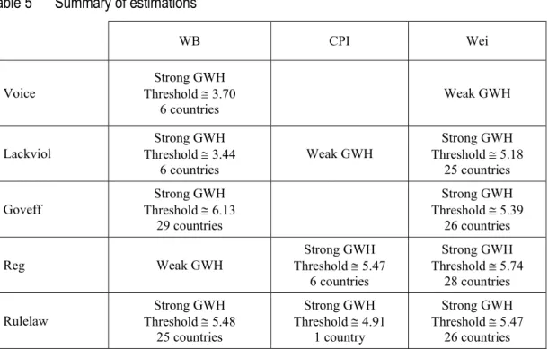
Table 5 Summary of estimations
WB CPI Wei Voice Strong GWH Threshold ≅ 3.70 6 countries Weak GWH Lackviol Strong GWH Threshold ≅ 3.44 6 countries Weak GWH Strong GWH Threshold ≅ 5.18 25 countries Goveff Threshold Strong GWH ≅ 6.13
29 countries Strong GWH Threshold ≅ 5.39 26 countries Reg Weak GWH Strong GWH Threshold ≅ 5.47 6 countries Strong GWH Threshold ≅ 5.74 28 countries Rulelaw Strong GWH Threshold ≅ 5.48 25 countries Strong GWH Threshold ≅ 4.91 1 country Strong GWH Threshold ≅ 5.47 26 countries
In a nutshell, out of the fifteen estimations that include an interaction term, ten show evi-dence of the strong form of the grease the wheels (GWH) hypothesis, three are consistent with the weak form of the grease the wheels hypothesis, and two show no sign of a rela-tionship between corruption and efficiency. None of them suggests a systematic detrimen-tal effect of corruption on aggregate efficiency. Furthermore, it must be pointed out that at least one estimation consistent with the strong form of the grease the wheels hypothesis can be found for each dimension of governance. All in all, we conclude there is clear evi-dence for some form of grease the wheels hypothesis.
An interesting by-product of our estimations is that they allow us to gauge the rela-tive importance of the interrelationship between corruption and each of the five dimensions of governance being analyzed.16 It appears then that government efficiency is clearly the most robust governance index in our sample. It is thus significantly associated with ineffi-ciency in all three baseline estimations and all three estimations that include an interaction with corruption. This is reassuring insofar as this is the aspect of governance that corrup-tion is theoretically meant to grease. On the other hand, voice and accountability performs worst of the various dimensions of governance. It only appears significant in one baseline estimation and two that include an interaction term. This finding is by and large consistent with the literature, where the correlation between democracy and economic outcomes usu-ally appears fragile.
Finally, all other indices only appear significant in one baseline estimation out of three, as well as in all estimations including an interaction term.
Our findings therefore contrast with previous empirical results that have in general supported a clear negative impact of corruption on economic performance, such as Mauro (1995), or Mo (2001). Most often they have not taken into account the non-linearity of the estimated relationship. Thus, it must be emphasized that we could achieve more usual results in our benchmark estimations where we did not control for the interaction of corruption with other dimensions of governance. While our results are clearly at odds with those of Méon and Sekkat (2005), where those interactions were specifically taken into ac-count, it should be noted that our estimations cannot be directly compared with their find-ings. Méon and Sekkat (2005) focused on the impact of corruption on growth and
invest-16 The results also underline differences between corruption indices. The results obtained with the World
Bank’s index and Wei’s index look very similar, while the CPI index stands out as slightly less robustly as-sociated with efficiency than the other two. Although we can offer no ready explanation for these differences, sample size may well play a role here.
score.
ment, while here we analyze aggregate efficiency. Also, their period of study is 1970-1998, while we have focused on 1994-1997.
5.2
A quantitative assessment
To get a feel of the quantitative significance of our results, let us focus on three countries from our sample whose government efficiency indicators differ (say, the Philippines, Tuni-sia, and Chile) and see what a reduction of corruption would imply for them. Our first country is plagued by a deficient government. The government efficiency index of our sec-ond country is close to the threshold estimated in Table 5. Our third country boasts a gov-ernment efficiency index well above the estimated threshold. We focus here on govern-ment efficiency as it is the most relevant dimension of governance for the grease the wheels hypothesis. (Of course, a similar exercise could be done with other indices.) Let us now assume that these countries succeed in bringing down corruption by one standard de-viation of the WB corruption index, i.e. two points. Such a reduction would approximately bring down the level of corruption to that of Italy for the Philippines, to that of Chile for Tunisia, and to that of the Netherlands for Chile.17
The coefficients estimated in estimation 4c.2 allow us to evaluate the impact of such a reduction of corruption on the aggregate efficiency of these three countries under study.18 To do so, the first step is to compute the overall coefficient of corruption for each country. With δ1 ≅ −0.4692 and δ2 ≅ 0.075, the overall coefficient of corruption reaches – 0.0668 in the Philippines, −0.0097 in Tunisia, and +0.092 in Chile, given their governance indices.19 The same reduction in the World Bank corruption index would therefore result in a different impact on efficiency, and hence income. Thus, given each country’s initial efficiency score and the quality of its government efficiency, the Philippines would witness a drop of 49.3 percentage points of its efficiency score, while Chile would see its effi-ciency score rise by 50.69 percentage points. The reduction of corruption will be accompa-nied by a small 5.76 percentage points reduction of Tunisia’s efficiency
17 The rescaled value of the WB corruption index is equal to 5.46 for the Philippines, 4.96 for Tunisia, and
2.94 for Chile. Following a two points reduction in their indices, those countries would respectively end up near Italy, whose index is 3.4, Chile, whose index is 2.94, and the Netherlands, whose index is equal to 0.94.
18 In fact, the estimated coefficients do not directly measure the first derivative of efficiency with respect to
corruption. Instead, they measure the derivative of ui, defined as ui = −log(efficiency). The variation of
effi-ciency can therefore be estimated asΔefficiency=(∂efficiency ∂ui)⋅Δui.
19 Recall that the coefficient of corruption in a country is a function of that country’s government efficiency.
The government efficiency index of the three countries under study is equal to 5.26 for the Philippines, 6.26 for Tunisia, and 7.34 for Chile.
Moreover, these variations in efficiency are synonymous to variations in output per worker since they reflect each country’s distance to the common production frontier.20 Thus, the Philippines’ output per worker would fall from US$1,567 to $795 per year, which is similar to that of Kenya. On the other hand, Chile’s output per worker would rise from $7,029 to $10,590 per year, bringing it close to Portugal. Finally, Tunisia’s output per worker would only rise marginally, from $4,081 to $4,316 per year. This is not surprising, since government effectiveness in Tunisia is very close to the threshold value. The coeffi-cient of corruption in that country is therefore very close to zero. At any rate, the main message of these simulations is that the impact of a reduction of corruption on output may be dramatic in countries where the governance index takes on extreme values.21 However, that impact varies wildly with the quality of the rest of the institutional framework, and can be either positive or negative.
5.3
Robustness checks
Although our results are obtained while controlling for several country-specific traits, we also consider it prudent to examine for a multi-colinearity problem. One might expect a positive correlation between, say, corruption and other governance indicators on the one hand, and the three control variables on the other. Thus, it can be argued that greater open-ness to trade may reduce corruption or improve the institutional framework as it encoura-ges ideas to circulate and subjects domestic practices to foreign scrutiny. One may also suspect ethnic fractionalization affects both institutions and economic performance through its impact on trust and social cohesion. Finally, geography and latitude may also affect both economic performance (as suggested by Sachs, 2001) and income as it historically determined the strategy of colonizers (see Acemoglu et al., 2001).
To check the robustness of our results to the choice of control variables, we there-fore run our estimations again, first dropping one control variable at a time, and then
drop-20 The simulated value of output can easily be simply computed as
0 i 1 i 0 i y efficiency efficiency = 1 i y .
21 While these orders of magnitude may seem huge, please recall that cross-country output level differences
pertain to the long term, as Hall and Jones (1999) remark. Also, the present orders of magnitude are in line with those reported in the literature. Mauro (1995) finds that a one standard deviation reduction in corruption can raise an economy’s growth rate by 0.8 points. After a couple of decades, this would result in a difference in its level of GDP comparable to the one that we describe here. Along similar lines, Hall and Jones (1999) observe that differences in institutional quality can account for a 25.2- to 38.4-fold difference in output per worker across countries.
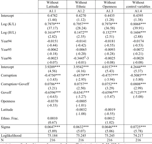
ping them all.22 As Table A1 in the appendix shows, our results are only slightly affected qualitatively and quantitatively.
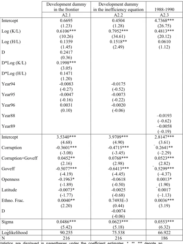
Another source of skepticism arises from the fact that our estimations do not dis-criminate between developed and developing countries. Pooling countries while ignoring development levels may neglect the fact that they may be operating along different produc-tion frontiers. In addiproduc-tion, the determinants of efficiency may differ across developed and developing countries. To address this issue, we split our sample into two equivalent subsets according to per capita income and created a dummy variable equal to one for every obser-vation where per capita income is greater than the median, and zero elsewhere. We then use this dummy variable in two ways. First, we interact it with production factor stocks and include the resulting interaction terms as well as the dummy variable itself into the expres-sion of the production frontier. This is equivalent to estimating a distinct production fron-tier for each sub-sample. The results presented in Table A2 of the appendix show that the coefficients of the corruption and governance indices are only slightly affected. Second, we add the dummy variable to the set of explanatory variables. The result of this estimation, also reported in Table A2, exhibits little influence on governance indicators. Our findings are therefore robust in distinguishing developed and developing countries.
We are also concerned that our results may be contingent on the period of study. We accordingly estimate the production frontier with data pertaining to the 1988-1990 pe-riod. That earlier period of time allows for an additional robustness check, which involves using a different dataset on output and capital per worker (i.e. the dataset in Easterly and Levine, 2001). Table A2 reports the results of these estimations. Once again, the coeffi-cients of the governance and corruption indices remain significant and exhibit signs consis-tent with the grease the wheels hypothesis.
Our final worry is that the results might be driven by the Cobb-Douglas specifica-tion of the producspecifica-tion frontier with constant returns to scale. We therefore test two alterna-tive specifications. The first is a translog production function specified as
ln (Y/L)it = α0 + α1 ln (K/L)it + α2 ln (H/L)it + α3[ln (K/L)it]2 + α4[ln (H/L)it]2
+ α5 ln (K/L)it ln (H/L)it + vit− uit . (4)
22 To save on space, we restrict ourselves to one index of corruption (the WB index) and one index of
institu-tional quality (government effectiveness, which is the most relevant to testing the grease the wheels hypothe-sis).
The second is a production frontier with variable returns to scale. Here, the production frontier is similar to the one presented in equation (1) if we except that production, physi-cal capital and human capital are not normalized by labor and that labor is added as a term in the frontier. The results of these estimations are displayed in Table A3. In both estima-tions, the coefficients of the corruption and governance indices remain similar to our pre-vious findings, both qualitatively and quantitatively. Our results are therefore robust to var-ious specifications of the production frontier.
These findings thus stand up to several robustness checks, leading to coefficients of the corruption and governance indices that are consistent with the grease the wheels hy-pothesis. Here, it must be stressed that their magnitude was systematically consistent with the strong form of the grease the wheels hypothesis, implying that corruption may lead to greater efficiency in some countries of the sample.
6
Concluding remarks
The present paper specifically tested the grease the wheels hypothesis against the sand the wheels hypothesis of corruption by focusing on aggregate efficiency. Unlike most previous studies, the results here provide no evidence of the sand the wheels hypothesis, but sub-stantial evidence of the grease the wheels hypothesis. Both weak and strong forms of the grease the wheels hypothesis were observed. Although it was repeatedly found that corrup-tion is less detrimental in countries where the rest of the institucorrup-tional framework is weaker, our estimations did not always imply that an increase in corruption may be beneficial in at least one country in the sample. However, for each of the five dimensions of governance taken into account, we find evidence of the strong grease the wheels hypothesis in at least one estimation.
A possible policy implication of these results is that countries plagued with ex-tremely inefficient institutional frameworks may benefit from allowing corruption to flour-ish. This interpretation, however, is risky. A country that would allow unfettered corrup-tion may eventually find itself with an even worse global institucorrup-tional framework, and thus be caught in a bad governance/low efficiency trap.
Encouraging countries to fight corruption, while also striving to improve other as-pects of governance, mainly government efficiency, is likely a more prudent policy
rec-ommendation we can draw from these findings. Moreover, a successful policy package should be multifaceted as narrow reform programs can be counter-productive. Ultimately, of course, the best policy choice for a given situation depends on the dynamics of the inter-relationship between corruption, governance, and economic performance, which are not fully understood yet. Understanding these dynamics should therefore feature highly on the political economy research agenda.
Appendix
A1 Countries in the sample
Australia, Austria, Belgium, Bolivia, Cameroon, Canada, Chile, Colombia; Costa Rica, Denmark, Ecuador, Egypt, El Salvador, Finland, France,