https://doi.org/10.1007/s11263-019-01158-4
Deep Affect Prediction in‑the‑Wild: Aff‑Wild Database and Challenge,
Deep Architectures, and Beyond
Dimitrios Kollias1 · Panagiotis Tzirakis1 · Mihalis A. Nicolaou1,2 · Athanasios Papaioannou1 · Guoying Zhao1,3 · Björn Schuller1 · Irene Kotsia1,4 · Stefanos Zafeiriou1,3
Received: 22 February 2018 / Accepted: 29 January 2019 © The Author(s) 2019
Abstract
Automatic understanding of human affect using visual signals is of great importance in everyday human–machine interac-tions. Appraising human emotional states, behaviors and reactions displayed in real-world settings, can be accomplished using latent continuous dimensions (e.g., the circumplex model of affect). Valence (i.e., how positive or negative is an emo-tion) and arousal (i.e., power of the activation of the emoemo-tion) constitute popular and effective representations for affect. Nevertheless, the majority of collected datasets this far, although containing naturalistic emotional states, have been captured in highly controlled recording conditions. In this paper, we introduce the Aff-Wild benchmark for training and evaluating affect recognition algorithms. We also report on the results of the First Affect-in-the-wild Challenge (Aff-Wild Challenge) that was recently organized in conjunction with CVPR 2017 on the Aff-Wild database, and was the first ever challenge on the estimation of valence and arousal in-the-wild. Furthermore, we design and extensively train an end-to-end deep neural architecture which performs prediction of continuous emotion dimensions based on visual cues. The proposed deep learning architecture, AffWildNet, includes convolutional and recurrent neural network layers, exploiting the invariant properties of convolutional features, while also modeling temporal dynamics that arise in human behavior via the recurrent layers. The AffWildNet produced state-of-the-art results on the Aff-Wild Challenge. We then exploit the AffWild database for learning features, which can be used as priors for achieving best performances both for dimensional, as well as categorical emo-tion recogniemo-tion, using the RECOLA, AFEW-VA and EmotiW 2017 datasets, compared to all other methods designed for the same goal. The database and emotion recognition models are available at http://ibug.doc.ic.ac.uk/resou rces/first -affec t-wild-chall enge.
Keywords Deep · Convolutional · Recurrent · Aff-Wild · Database · Challenge · In-the-wild · Facial · Dimensional ·
Categorical · Emotion · Recognition · Valence · Arousal · AffWildNet · RECOLA · AFEW · AFEW-VA · EmotiW
Communicated by Xiaoou Tang. * Dimitrios Kollias [email protected] Panagiotis Tzirakis [email protected] Mihalis A. Nicolaou [email protected] Athanasios Papaioannou [email protected] Guoying Zhao [email protected] Björn Schuller [email protected] Irene Kotsia [email protected] Stefanos Zafeiriou [email protected]
1 Queens Gate, London SW7 2AZ, UK
2 Department of Computing, Goldsmiths University
of London, London SE14 6NW, UK
3 Center for Machine Vision and Signal Analysis, University
of Oulu, Oulu, Finland
4 Department of Computer Science, Middlesex University
1 Introduction
Current research in automatic analysis of facial affect aims at developing systems, such as robots and virtual humans, that will interact with humans in a naturalistic way under real-world settings. To this end, such systems should auto-matically sense and interpret facial signals relevant to emo-tions, appraisals and intentions. Moreover, since real-world settings entail uncontrolled conditions, where subjects oper-ate in a diversity of contexts and environments, systems that perform automatic analysis of human behavior should be robust to video recording conditions, the diversity of con-texts and the timing of display.1
For the past twenty years research in automatic analysis of facial behavior was mainly limited to posed behavior which was captured in highly controlled recording conditions (Pan-tic et al. 2005; Valstar and Pantic 2010; Tian et al. 2001; Lucey et al. 2010). Some representative datasets, which are still used in many recent works (Jung et al. 2015), are the Cohn–Kanade database (Tian et al. 2001; Lucey et al. 2010), MMI database (Pantic et al. 2005; Valstar and Pantic 2010), Multi-PIE database (Gross et al. 2010) and the BU-3D and BU-4D databases (Yin et al. 2006, 2008).
Nevertheless, it is now accepted by the community that the facial expressions of naturalistic behaviors can be radi-cally different from the posed ones (Corneanu et al. 2016; Sariyanidi et al. 2015; Zeng et al. 2009). Hence, efforts have been made in order to collect subjects displaying naturalistic behavior. Examples include the recently collected EmoPain (Aung et al. 2016) and UNBC-McMaster (Lucey et al. 2011) databases for analysis of pain, the RU-FACS database of subjects participating in a false opinion scenario (Bartlett et al. 2006) and the SEMAINE corpus (McKeown et al.
2012) which contains recordings of subjects interacting with a Sensitive Artificial Listener (SAL) in controlled condi-tions. All the above databases have been captured in well-controlled recording conditions and mainly under a strictly defined scenario eliciting pain.
Representing human emotions has been a basic topic of research in psychology. The most frequently used emotion representation is the categorical one, including the seven basic categories, i.e., Anger, Disgust, Fear, Happiness, Sadness, Surprise and Neutral (Dalgleish and Power 2000; Cowie and Cornelius 2003). It is, however, the dimensional emotion representation (Whissel 1989; Russell 1978) which is more appropriate to represent subtle, i.e., not only extreme, emotions appearing in everyday human computer interactions. To this end, the 2-D valence and arousal space
is the most usual dimensional emotion representation. Fig-ure 1 shows the 2-D Emotion Wheel (Plutchik 1980), with valence ranging from very positive to very negative and arousal ranging from very active to very passive.
Some emotion recognition databases exist in the litera-ture that utilize dimensional emotion representation. Exam-ples are the SAL (Douglas-Cowie et al. 2008), SEMAINE (McKeown et al. 2012), MAHNOB-HCI (Soleymani et al.
2012), Belfast naturalistic,2 Belfast induced (Sneddon et al.
2012), DEAP (Koelstra et al. 2012), RECOLA (Ringeval et al. 2013), SEWA3 and AFEW-VA (Kossaifi et al. 2017)
databases.
Currently, there are many challenges (competitions) in the behavior analysis domain. One such example is the Audio/ Visual Emotion Challenges (AVEC) series (Valstar et al.
2013, 2014, 2016; Ringeval et al. 2015, 2017) which started in 2011. The first challenge (Schuller et al. 2011) used the SEMAINE database for classification purposes by binarizing its continuous values, while the second challenge (Schuller et al. 2012) used the same database but with its original values. The last challenge (Ringeval et al. 2017) utilized the SEWA database. Before this and for two consecutive years (Ringeval et al. 2015; Valstar et al. 2016) the RECOLA dataset was used.
However these databases have some of the below limita-tions, as shown in Table 1:
(1) They contain data recorded in laboratory or controlled environments.
(2) Their diversity is limited due to the small total number of subjects they contain, the limited amount of head pose variations and present occlusion, the static back-ground or uniform illumination
(3) The total duration of their included videos is rather short
To tackle the aforementioned limitations, we collected the first, to the best of our knowledge, large scale captured in-the-wild database and annotated it in terms of valence and arousal. To do so, we capitalized on the abundance of data available in video-sharing websites, such as YouTube (2011)4 and selected videos that display the affective
behav-ior of people, for example videos that display the behavbehav-ior
1 It is well known that the interpretation of a facial expression may
depend on its dynamics, e.g. posed versus spontaneous expressions (Zeng et al. 2009).
2 https ://belfa st-natur alist ic-db.sspne t.eu/. 3 http://sewap rojec t.eu.
4 The collection has been conducted under the scrutiny and approval
of the Imperial College Ethical Committee (ICREC). The majority of the chosen videos were under Creative Commons License (CCL). For those videos that were not under CCL, we have contacted the per-son who created them and asked for their approval to be used in this research.
Fig. 1 The 2-D Emotion Wheel
Table 1 Databases annotated for both valence and arousal and their attributes
Database No. of subjects No. of videos Duration of each video Condition
MAHNOB-HCI (Soleymani et al. 2012) 27 20 34.9–117 s Controlled
DEAP (Koelstra et al. 2012) 32 40 1 min Controlled
AFEW-VA (Kossaifi et al. 2017) < 600 600 0.5–4 s In-the-wild
SAL (Douglas-Cowie et al. 2008) 4 24 25 min Controlled
SEMAINE (McKeown et al. 2012) 150 959 5 min Controlled
Belfast naturalistic (see Footnote 2) 125 298 10–60 s Controlled
Belfast induced (Sneddon et al. 2012) 37 37 5–30 s Controlled
RECOLA (Ringeval et al. 2013) 46 46 5 min Controlled
of people when watching a trailer, a movie, a disturbing clip, or reactions to pranks.
To this end we have collected 298 videos displaying reactions of 200 subjects, with a total video duration of more than 30 h. This database has been annotated by 8 lay experts with regards to two continuous emotion dimensions, i.e. valence and arousal. We then organized the Aff-Wild Challenge based on the Aff-Wild database (Zafeiriou et al.
2017; Kollias et al. 2017), in conjunction with International Conference on Computer Vision and Pattern Recognition (CVPR) 2017. The participating teams submitted their results to the challenge, outperforming the provided base-line. However, as described later in this paper, the achieved performances were rather low.
For this reason, we capitalized on the Aff-Wild database to build CNN and CNN plus RNN architectures shown to achieve excellent performance on this database, outperform-ing all previous participants’ performances. We have made extensive experimentations, testing structures for combining convolutional and recurrent neural networks and training them altogether as an end-to-end architecture. We have used a loss function that is based on the Concordance Correla-tion Coefficient (CCC), which we also compare it with the usual Mean Squared Error (MSE) criterion. Additionally, we appropriately fused, within the network structures, two types of inputs, the 2-D facial images—presented at the input of the end-to-end architecture—and the 2-D facial landmark positions—presented at the 1st fully connected layer of the architecture.
We have also investigated the use of the created CNN-RNN architecture for valence and arousal estimation in other datasets, focusing on the RECOLA and the AFEW-VA ones. Last but not least, taking into consideration the large in-the-wild nature of this database, we show that our network can be also used for other emotion recognition tasks, such as classification of the universal expressions.
The only challenge, apart from last AVEC (2017) (Rin-geval et al. 2017), using ‘in-the-wild’ data is the series of EmotiW (Dhall et al. 2013, 2014, 2015, 2016, 2017). It uses the AFEW dataset, whose samples come from movies, TV shows and series. To the best of our knowledge, this is the first time that a dimensional database and features extracted from it, are used as priors for categorical emotion recogni-tion in-the-wild, exploiting the EmotiW Challenge dataset. To summarize, there exist several databases for dimen-sional emotion recognition. However, they have limitations, mostly due to the fact that they are not captured in-the-wild (i.e., not in uncontrolled conditions). This urged us to create the benchmark Aff-Wild database and organize the Aff-Wild Challenge. The results acquired are presented later in full detail. We proceeded in conducting experiments and build-ing CNN and CNN plus RNN architectures, includbuild-ing the AffWildNet, producing state-of-the-art results.
The main contributions of the paper are the following:
• It is the first time that a large in-the-wild database—with a big variety of: (1) emotional states, (2) rapid emotional changes, (3) ethnicities, (4) head poses, (5) illumination conditions and (6) occlusions—has been generated and used for emotion recognition.
• An appropriate state-of-the-art deep neural network (DNN) (AffWildNet) has been developed, which is capa-ble of learning to model all these phenomena. This has not been technically straightforward, as can be verified by comparing the AffWildNet’s performance to the per-formances of other DNNs developed by other research groups which participated in the Aff-Wild Challenge.
• It is shown that the AffWildNet has been capable of generalizing its knowledge in other emotion recognition datasets and contexts. By learning complex and emotion-ally rich features of the AffWild, the AffWildNet consti-tutes a robust prior for both dimensional and categorical emotion recognition. To the best of our knowledge, it is the first time that state-of-the-art performances are achieved in this way.
The rest of the paper is organized as follows. Section 2
presents the databases generated and used in the presented experiments. Section 3 describes the pre-processing and annotation methodologies that we used. Section 4 begins by describing the Aff-Wild Challenge that was organized, the baseline method, the methodologies of the participating teams and their results. It then presents the end-to-end DNNs which we developed and the best performing AffWildNet architecture. Finally experimental studies and results are presented and discussed, illustrating the above develop-ments. Section 5 describes how the AffWildNet can be used as a prior for other, both dimensional and categorical, emo-tion recogniemo-tion problems yielding state-of-the-art results. Finally, Sect. 6 presents the conclusions and future work following the reported developments.
2 Existing Databases
We briefly present the RECOLA, AFEW, AFEW-VA data-bases used for emotion recognition and mention their limi-tations which lead to the creation of the Aff-Wild database. Table 2 summarizes these limitations, also showing the superior properties of Aff-Wild.
2.1 RECOLA Dataset
The REmote COLlaborative and Affective (RECOLA) data-base was introduced by Ringeval et al. (2013) and it contains natural and spontaneous emotions in the continuous domain
(arousal and valence). The corpus includes four modali-ties: audio, visual, electro-dermal activity and electro-car-diogram. It consists of 46 French speaking subjects being recorded for 9.5 h recordings in total. The recordings were annotated for 5 min each by 6 French-speaking annotators (three male, three female). The dataset is divided into three parts, namely, training (16 subjects), validation (15 subjects) and test (15 subjects), in such a way that the gender, age and mother tongue are stratified (i.e., balanced).
The main limitations of this dataset include the tightly controlled laboratory environment, as well as the small num-ber of subjects. It should be also noted that it contains a moderate total number of frames.
2.2 The AFEW Dataset
The series of EmotiW challenges (Dhall et al. 2013, 2014,
2015, 2016, 2017) make use of the data from the Acted Facial Expression In The Wild (AFEW) dataset (Dhall et al.
2017). This dataset is a dynamic temporal facial expressions data corpus consisting of close to real world scenes extracted from movies and reality TV shows. In total it contains 1809 videos. The whole dataset is split into three sets: training set (773 video clips), validation set (383 video clips) and test set (653 video clips). It should be emphasized that both train-ing and validation sets are mainly composed of real movie records, however 114 out of 653 video clips in the test set are real TV clips, thus increasing the difficulty of the challenge. The number of subjects is more than 330, aged 1–77 years. The annotation is according to 7 facial expressions (Anger, Disgust, Fear, Happiness, Neutral, Sadness and Surprise) and is performed by three annotators. The EmotiW chal-lenges focus on audiovisual classification of each clip into the seven basic emotion categories.
The limitations of the AFEW dataset include its small size (in terms of total number of frames) and its restriction to only seven emotion categories, some of which (fear, disgust, surprise) include a small number of samples.
2.3 The AFEW‑VA Database
Very recently, a part of the AFEW dataset of the series of EmotiW challenges has been annotated in terms of valence and arousal, thus creating the so called AFEW-VA (Kossaifi et al. 2017) database. In total, it contains 600 video clips that were extracted from feature films and simulate real-world conditions, i.e., occlusions, different illumination conditions and free movements from subjects. The videos range from short (around 10 frames) to longer clips (more than 120 frames). This database includes per-frame annotations of valence and arousal. In total, more than 30,000 frames were annotated for dimensional affect prediction of arousal and valence, using discrete values in the range of [ −10 , +10].
The database’s limitations include its small size (in terms of total number of frames), the small number of annota-tors (only 2) and the use of discrete values for valence and arousal. It should be noted that the 2-D Emotion Wheel (Fig. 1) is a continuous space. Therefore, using discrete only values for valence and arousal provides a rather coarse approximation of the behavior of persons in their everyday interactions. On the other hand, using continuous values can provide improved modeling of the expressiveness and rich-ness of emotional states met in everyday human behaviors.
2.4 The Aff‑Wild Database
We created a database consisting of 298 videos, with a total length of more than 30 h. The aim was to collect sponta-neous facial behaviors in arbitrary recording conditions.
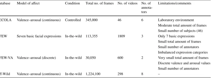
Table 2 Current databases used for emotion recognition in this paper, their attributes and limitations compared to Aff-Wild
Database Model of affect Condition Total no. of frames No. of videos No. of annota-tors
Limitations/comments RECOLA Valence–arousal (continuous) Controlled 345,000 46 6 Laboratory environment
Moderate total amount of frames Small number of subjects (46) AFEW Seven basic facial expressions In-the-wild 113,355 1809 3 Only 7 basic expressions
Small total amount of frames Small number of annotators Imbalanced expression categories AFEW-VA Valence–arousal (discrete) In-the-wild 30,050 600 2 Very small total amount of frames
Discrete valence and arousal values Small number of annotators Aff-Wild Valence–arousal (continuous) In-the-wild 1,224,100 298 8 –
To this end, the videos were collected using the Youtube video sharing web-site. The main keyword that was used to retrieve the videos was “reaction”. The database dis-plays subjects reacting to a variety of stimuli, e.g. view-ing an unexpected plot twist of a movie or series, a trailer of a highly anticipated movie, or tasting something hot or disgusting. The subjects display both positive or negative emotions (or combinations of them). In other cases, subjects display emotions while performing an activity (e.g., riding a rolling coaster). In some videos, subjects react on a practi-cal joke, or on positive surprises (e.g., a gift). The videos contain subjects from different genders and ethnicities with high variations in head pose and lightning.
Most of the videos are in YUV 4:2:0 format, with some of them being in AVI format. Eight subjects have annotated the videos following a methodology similar to the one proposed in Cowie et al. (2000), in terms of valence and arousal. An online annotation procedure was used, according to which annotators were watching each video and provided their annotations through a joystick. Valence and arousal range
continuously in [ −1 , +1 ]. All subjects present in each video have been annotated. The total number of subjects is 200, with 130 of them being male and 70 of them female. Table 3
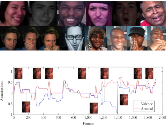
shows the general attributes of the Aff-Wild database. Fig-ure 2 shows some frames from the Aff-Wild database, with people from different ethnicities displaying various emo-tions, with different head poses and illumination condiemo-tions, as well as occlusions in the facial area.
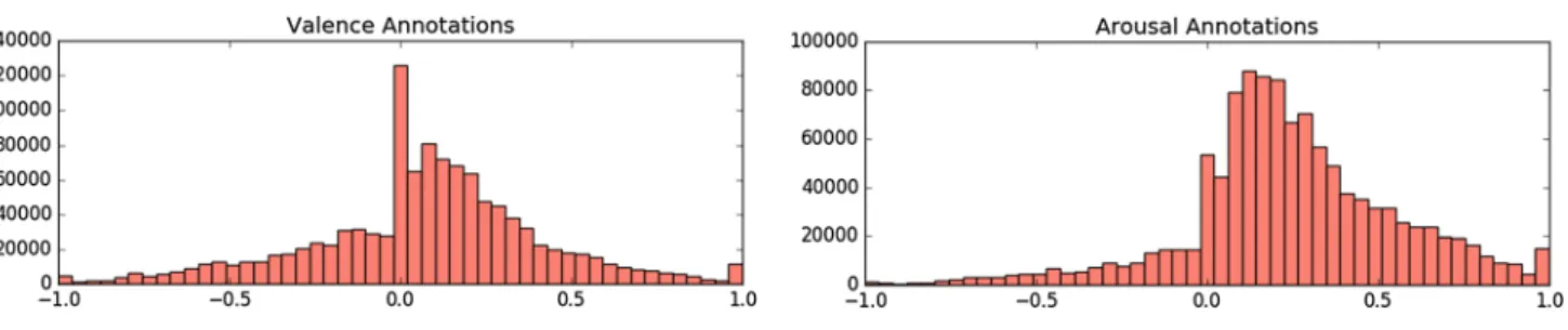
Figure 3 shows an example of annotated valence and arousal values over a part of a video in the Aff-Wild, together with corresponding frames. This illustrates the in-the-wild nature of our database, namely, including many different emotional states, rapid emotional changes and occlusions in the facial areas. Figure 3 also shows the use of continuous values for valence and arousal annotation, which gives the ability to effectively model all these different phenomena. Figure 4 provides a histogram for the annotated values for valence and arousal in the generated database.
3 Data Pre‑processing and Annotation
In this section we describe the pre-processing process of the Aff-Wild videos so as to perform face and facial land-mark detection. Then we present the annotation procedure including:
(1) Creation of the annotation tool.
(2) Generation of guidelines for six experts to follow in order to perform the annotation.
Fig. 2 Frames from the
Aff-Wild database which show subjects in different emotional states, of different ethnicities, in a variety of head poses, illumination conditions and occlusions
Table 3 Attributes of the Aff-Wild database
Attribute Description
Length of videos 0.10–14.47 min
Video format AVI , MP4
Average Image Resolution (AIR) 607×359
Standard deviation of AIR 85×11
Median Image Resolution 640×360
Fig. 3 Valence and arousal
annotations over a part of a video, along with correspond-ing frames; illustratcorrespond-ing (i) the in-the-wild nature of Aff-Wild (different emotional states, rapid emotional changes, occlusions) and (ii) the use of continuous values for valence and arousal
0 200 400 600 800 1,000 1,200 1,400 1,600 1,800 2,000 −1 −0.5 0 0.5 1 Frames Annotations Valence Arousal
(3) Post-processing annotation: the six annotators watched all videos again, checked their annotations and per-formed any corrections; two new annotators watched all videos and selected 2–4 annotations that best described each video; final annotations are the mean of the selected annotations by these two new annota-tors.
The detected faces and facial landmarks, as well as the gen-erated annotations are publicly available with the Aff-Wild database.
Finally, we present a statistical analysis of the annotations created for each video, illustrating the consistency of annota-tions achieved by using the above procedure.
3.1 Aff‑Wild Video Pre‑processing
VirtualDub (Lee 2002) was used first so as to trim the raw YouTube videos, mainly at their beginning and end-points, in order to remove useless content (e.g., advertisements). Then, we extracted a total of 1,224,100 video frames using the Menpo software (Alabort-i-Medina et al. 2014). In each frame, we detected the faces and generated corresponding bounding boxes, using the method described in Mathias et al. (2014). Next, we extracted facial landmarks in all frames using the best performing method as indicated in Chrysos et al. (2018).
During this process, we removed frames in which the bounding box or landmark detection failed. Failures occurred when either the bounding boxes, or landmarks, were wrongly detected, or were not detected at all. The for-mer case was semi-automatically discovered by: (i) detecting significant shifts in the bounding box and landmark positions between consecutive frames and (ii) having the annotators verify the wrong detection in the frames.
3.2 Annotation Tool
For data annotation, we developed our own application that builds on other existing ones, like Feeltrace (Cowie et al.
2000) and Gtrace (Cowie et al. 2012). A time-continuous
annotation is performed for each affective dimension, with the annotation process being as follows:
(a) The user logs in to the application using an identifier (e.g. his/her name) and selects an appropriate joystick; (b) A scrolling list of all videos appears and the user selects
a video to annotate;
(c) A screen appears that shows the selected video and a slider of valence or arousal values ranging in [−1, 1]; (d) The user annotates the video by moving the joystick
either up or down;
(e) Finally, a file is created including the annotation values and the corresponding time instances that the annota-tions are generated.
It should be mentioned that the time instances generated in the above step (e), did not generally match the video frame rate. To tackle this problem, we modified/re-sam-pled the annotation time instances using nearest neighbor interpolation.
Figure 5 shows the graphical interface of our tool when annotating valence (the interface for arousal is similar); this corresponds to step (c) of the above described annotation process.
Fig. 4 Histogram of valence and arousal annotations of the Aff-Wild database
Fig. 5 The GUI of the annotation tool when annotating valence (the
It should also be added that the annotation tool has also the ability to show the inserted valence and arousal annota-tion while displaying a respective video. This is used for annotation verification in a post-processing step.
3.3 Annotation Guidelines
Six experts were chosen to perform the annotation task. Each annotator was instructed orally and through a multi-page document on the procedure to follow for the task. This docu-ment included a list of some well identified emotional cues for both arousal and valence, providing a common basis for the annotation task. On top of that the experts used their own appraisal of the subject’s emotional state for creating the annotations.5 Before starting the annotation of each video,
the experts watched the whole video so as to know what to expect regarding the emotions being displayed in the video.
3.4 Annotation Post‑processing
A post-processing annotation verification step was also performed. Every expert-annotator watched all videos for a second time in order to verify that the recorded annotations were in accordance with the shown emotions in the videos or change the annotations accordingly. In this way, a further validation of annotations was achieved.
After the annotations have been validated by the annota-tors, a final annotation selection step followed. Two new experts watched all videos and, for every video, selected the annotations (between two and four) which best described the
displayed emotions. The mean of these selected annotations constitute the final Aff-Wild labels.
This step is significant for obtaining highly correlated annotations, as shown by the statistical analysis presented next.
3.5 Statistical Analysis of Annotations
In the following we provide a quantitative and rich statisti-cal analysis of the achieved Aff-Wild labeling. At first, for each video, and independently for valence and arousal, we computed:
(i) The inter-annotator correlations, i.e., the correlations of each one of the six annotators with all other anno-tators, which resulted in five correlation values per annotator;
(ii) For each annotator, his/her average inter-annotator correlations, resulting in one value per annotator; the mean of those six average inter-annotator correla-tions value is denoted next as MAC-A;
(iii) The average inter-annotator correlations, across only the selected annotators, as described in the previous subsection, resulting in one value per selected anno-tator; the mean of those 2–4 average inter-selected-annotator correlations values is denoted next as MAC-S.
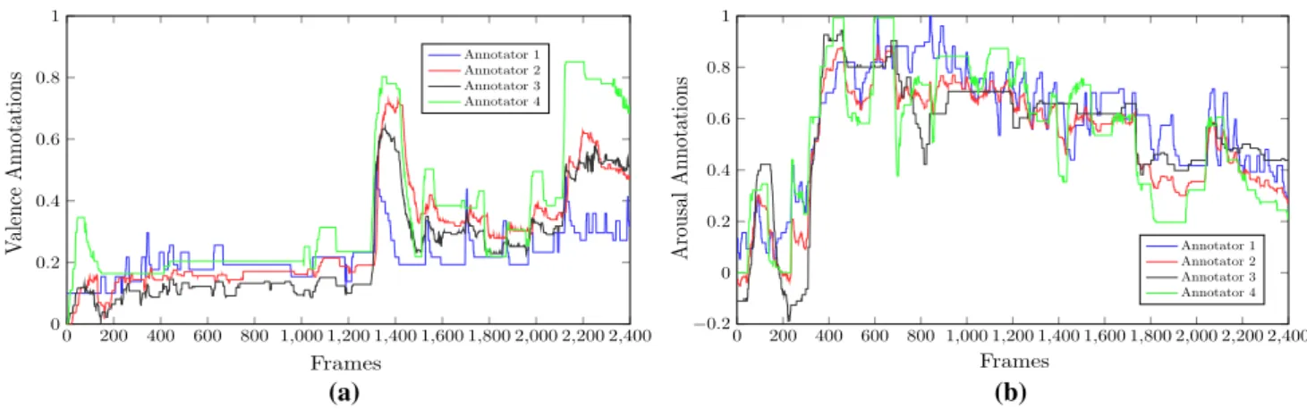
We then computed over all videos and independently for valence and arousal, the mean of MAC-A and the mean of MAC-S computed in (ii) and (iii) above. The mean MAC-A is 0.47 for valence and 0.46 for arousal, whilst the mean MAC-S for valence is 0.71 and for arousal 0.70. An example set of annotations is shown in Fig. 6, in an effort to fur-ther clarify the obtained MAC-S values. It shows the four selected annotations in a video segment for valence and
0 200 400 600 800 1,000 1,200 1,400 1,600 1,800 2,000 2,200 2,400 0 0.2 0.4 0.6 0.8 1 Frames Valence Annotations Annotator 1 Annotator 2 Annotator 3 Annotator 4 (a) 0 200 400 600 800 1,000 1,200 1,400 1,600 1,800 2,000 2,200 2,400 −0.2 0 0.2 0.4 0.6 0.8 1 Frames Arousal Annotation s Annotator 1 Annotator 2 Annotator 3 Annotator 4 (b)
Fig. 6 The four selected annotations in a video segment for a valence and b arousal. In both cases, the value of MAC-S (mean of average
corre-lations between these four annotations) is 0.70. This value is similar to the mean MAC-S obtained over all Aff-Wild
5 All annotators were computer scientists who were working on
face analysis problems and all had a working understanding of facial expressions.
arousal, respectively, with MAC-S value of 0.70 (similar to the mean MAC-S value obtained over all Aff-Wild).
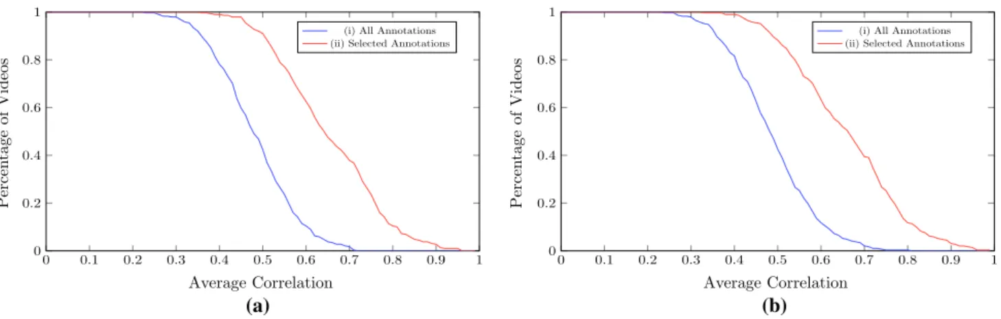
In addition, Fig. 7 shows the cumulative distribution of MAC-S and MAC-A values over all Aff-Wild videos for valence (Fig. 7a) and arousal (Fig. 7b). In each case, two curves are shown. Every point (x, y) on these curves has a
y value showing the percentage of videos with a (i) MAC-S (red curve) or (ii) MAC-A (blue curve) value greater or equal to x; the latter denotes an average correlation in [0, 1]. It can be observed that the mean MAC-S value, corresponding to a value of 0.5 in the vertical axis, is 0.71 for valence and 0.70 for arousal. These plots also illustrate that the MAC-S values are much higher than the corresponding MAC-A values in both valence and arousal annotation, verifying the effective-ness of the annotation post-processing procedure.
Next, we conducted similar experiments for the valence/ arousal average annotations and the facial landmarks in each video, in order to evaluate the correlation of annotations to landmarks. To this end, we utilized Canonical Correlation Analysis (CCA) (Hardoon et al. 2003). In particular, for each video and independently for valence and arousal, we computed the correlation between landmarks and the average of (i) all or (ii) selected annotations.
Figure 8 shows the cumulative distribution of these cor-relations over all Aff-Wild videos for valence (Fig. 8a) and arousal (Fig. 8b), similarly to Fig. 7. Results of this analy-sis verify that the annotator-landmark correlation is much higher in the case of selected annotations than in the case of all annotations. 0 0.1 0.2 0.3 0.4 0.5 0.6 0.7 0.8 0.9 1 0 0.2 0.4 0.6 0.8 1 Average Correlation Pe rcen tage of Videos
All Annotators (MAC-A) Selected Annotators (MAC-S)
(a) 0 0.1 0.2 0.3 0.4 0.5 0.6 0.7 0.8 0.9 1 0 0.2 0.4 0.6 0.8 1 Average Correlation Percen tage of Videos
All Annotators (MAC-A) Selected Annotators (MAC-S)
(b)
Fig. 7 The cumulative distribution of MAC-S (mean of average
selected-annotator correlations) and MAC-A (mean of average inter-annotator correlations) values over all Aff-Wild videos for valence (a) and arousal (b). The Figure shows the percentage of videos with
a MAC-S/MAC-A value greater or equal to the values shown in the horizontal axis. The mean MAC-S value, corresponding to a value of 0.5 in the vertical axis, is 0.71 for valence and 0.70 for arousal
0 0.1 0.2 0.3 0.4 0.5 0.6 0.7 0.8 0.9 1 0 0.2 0.4 0.6 0.8 1 Average Correlation Percen tage of Videos Percen tage of Videos
(i) All Annotations (ii) Selected Annotations
(a) 0 0.1 0.2 0.3 0.4 0.5 0.6 0.7 0.8 0.9 1 0 0.2 0.4 0.6 0.8 1 Average Correlation
(i) All Annotations (ii) Selected Annotations
(b)
Fig. 8 The cumulative distribution of the correlation between
land-marks and the average of (i) all or (ii) selected annotations over all Aff-Wild videos for valence (a) and arousal (b). The figure shows the
percentage of videos with a correlation value greater or equal to the values shown in the horizontal axis
4 Developing the AffWildNet
This section begins by presenting the first Aff-Wild Chal-lenge that was organized based on the Aff-Wild database and held in conjunction with CVPR 2017. It includes short descriptions and results of the algorithms of the six research groups that participated in the challenge. Although the results are promising, there is much room for improvement.
For this reason we developed our own CNN and CNN plus RNN architectures based on the Aff-Wild database. We propose the AffWildNet as the best performing among the developed architectures. Our developments, ablation studies and discussions are presented next.
4.1 The Aff‑Wild Challenge
The training data (i.e., videos and annotations) of the Aff-Wild challenge were made publicly available on the 30th of January 2017, followed by the release of the test videos (without annotations). The participants were given the free-dom to split the data into train and validation sets, as well as to use any other dataset. The maximum number of submitted entries for each participant was three. Table 4 summarizes the specific attributes (numbers of males, females, videos, frames) of the training and test sets of the challenge.
In total, ten different research groups downloaded the Aff-Wild database. Six of them made experiments and submitted their results to the workshop portal. Based on the perfor-mance they obtained on the test data, three of them were selected to present their results to the workshop.
Two criteria were considered for evaluating the perfor-mance of the networks. The first one is Concordance Cor-relation Coefficient (CCC) (Lawrence and Lin 1989), which is widely used in measuring the performance of dimensional emotion recognition methods, e.g., the series of AVEC chal-lenges. CCC evaluates the agreement between two time series (e.g., all video annotations and predictions) by scaling their correlation coefficient with their mean square differ-ence. In this way, predictions that are well correlated with the annotations but shifted in value are penalized in propor-tion to the deviapropor-tion. CCC takes values in the range [−1, 1] , where +1 indicates perfect concordance and −1 denotes per-fect discordance. The highest the value of the CCC the better the fit between annotations and predictions, and therefore high values are desired. The mean value of CCC for valence
and arousal estimation was adopted as the main evaluation criterion. CCC is defined as follows:
where 𝜌xy is the Pearson Correlation Coefficient (Pearson
CC), sx and sy are the variances of all video valence/arousal
annotations and predicted values, respectively and sxy is the corresponding covariance value.
The second criterion is the Mean Squared Error (MSE), which is defined as follows:
where x and y are the (valence/arousal) annotations and pre-dictions, respectively, and N is the total number of samples. The MSE gives us a rough indication of how the derived emotion model is behaving, providing a simple comparative metric. A small value of MSE is desired.
4.1.1 Baseline Architecture
The baseline architecture for the challenge was based on the CNN-M (Chatfield et al. 2014) network, as a simple model that could be used to initiate the procedure. In particular, our network used the convolutional and pooling parts of CNN-M having been trained on the FaceValue dataset (Albanie and Vedaldi 2016). On top of that we added one 4096-fully con-nected layer and a 2-fully concon-nected layer that provides the valence and arousal predictions. The interested reader can refer to “Appendix A” for a short description and the struc-ture of this architecstruc-ture.
The input to the network were the facial images resized to resolution of 224×224×3 , or 96×96×3 , with the inten-sity values being normalized to the range [−1, 1].
In order to train the network, we utilized the Adam opti-mizer algorithm; the batch size was set to 80, and the initial learning rate was set to 0.001. Training was performed on a single GeForce GTX TITAN X GPU and the training time was about 4–5 days. The platform used for this implementa-tion was Tensorflow (Abadi et al. 2016).
4.1.2 Participating Teams’ Algorithms
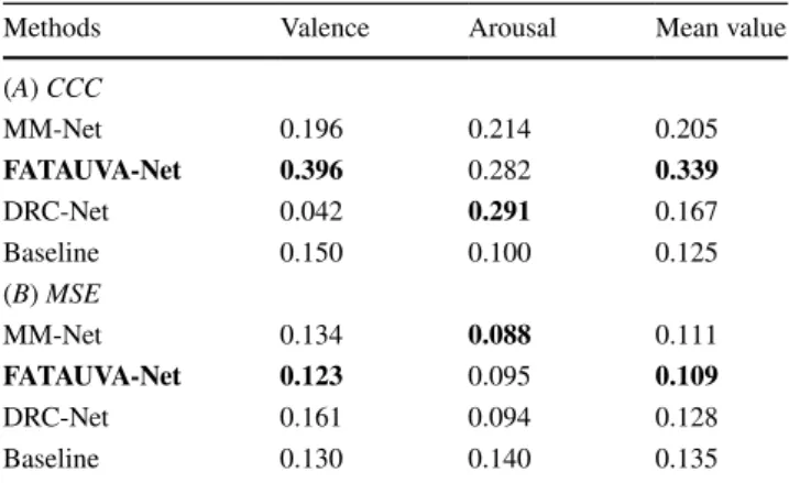
The three papers accepted to this challenge are briefly reported below, while Table 5 compares the acquired results (in terms of CCC and MSE) by all three methods and the baseline network. As one can see, FATAUVA-Net (Chang et al. 2017) has provided the best results in terms of the mean CCC and mean MSE for valence and arousal.
(1) 𝜌c= 2sxy s2 x+s 2 y+ (x̄−y)̄ 2 = 2sxsy𝜌xy s2 x+s 2 y+ (x̄−y)̄ 2, (2) MSE= 1 N N ∑ i=1 (xi−yi)2,
Table 4 Attributes of training and test sets of Aff-Wild
Set No. of males No. of
females No. of videos Total No. of frames
Training 106 48 252 1,008,650
We should note that after the end of the challenge, more groups enquired about the Aff-Wild database and sent results for evaluation, but here we report only on the teams that participated in the challenge.
In the MM-Net method (Li et al. 2017), a variation of a deep convolutional residual neural network (ResNet) (He et al. 2016) is first presented for affective level estimation of facial expressions. Then, multiple memory networks are used to model temporal relations between the video frames. Finally, ensemble models are used to combine the predic-tions of the multiple memory networks, showing that the latter steps improve the initially obtained performance, as far as MSE is concerned, by more than 10%.
In the FATAUVA-Net method (Chang et al. 2017), a deep learning framework is presented, in which a core layer, an attribute layer, an action unit (AU) layer and a valence–arousal layer are trained sequentially. The core layer is a series of convolutional layers, followed by the attribute layer which extracts facial features. These layers are applied to supervise the learning of AUs. Finally, AUs are employed as mid-level representations to estimate the intensity of valence and arousal.
In the DRC-Net method (Mahoor and Hasani 2017), three neural network-based methods which are based on Inception-ResNet (Szegedy et al. 2017) modules redesigned specifically for the task of facial affect estimation are presented and com-pared. These methods are: Shallow Inception-ResNet, Deep Inception-ResNet, and Inception-ResNet with Long Short Term Memory (Hochreiter and Schmidhuber 1997). Facial features are extracted in different scales and both, the valence and arousal, are simultaneously estimated in each frame. Best results are obtained by the Deep Inception-ResNet method.
All participants applied deep learning methods to the problem of emotion analysis of the video inputs. The
following conclusions can be drawn from the reported results. First, CCC of arousal predictions was really low for all three methods. Second, MSE of valence predictions was high for all three methods and CCC was low, except for the winning method. This illustrates the difficulty in recogniz-ing emotion in-the-wild, where, for instance, illumination conditions differ, occlusions are present and different head poses are met.
4.2 Deep Neural Architectures and Ablation Studies
Here, we present our developments and ablation studies towards designing deep CNN and CNN plus RNN architec-tures for the Aff-Wild. We present the proposed architecture, AffWildNet, which is a CNN plus RNN network that pro-duced the best results in the database.
4.2.1 The Roadmap
A. We considered two network settings:
(1) A CNN network trained in an end-to-end man-ner, i.e., using raw intensity pixels, to produce 2-D predictions of valence and arousal,
(2) A RNN stacked on top of the CNN to capture tem-poral information in the data, before predicting the affect dimensions; this was also trained in an end-to-end manner.
To extract features from the frames we experimented with three CNN architectures, namely, ResNet-50, VGG-Face (Parkhi et al. 2015) and VGG-16 (Simon-yan and Zisserman 2014). To consider the contextual information in the data (RNN case) we experimented with both the Long Short-Term Memory (LSTM) and the Gated Recurrent Unit (GRU) (Chung et al. 2014) architectures.
B. To further boost the performance of the networks, we also experimented with the use of facial landmarks. Here we should note that the facial landmarks are provided on-the-fly for training and testing the networks. The fol-lowing two scenarios were tested:
(1) The networks were applied directly on cropped facial video frames of the generated database. (2) The networks were trained on both the facial video
frames as well as the facial landmarks correspond-ing to the same frame.
C. Since the main evaluation criterion of the Aff-Wild Challenge was the mean value of CCC for valence and arousal, our loss function was based on that criterion and was defined as:
Table 5 Concordance Correlation Coefficient (CCC) and Mean
Squared Error (MSE) of valence and arousal predictions provided by the methods of the three participating teams and the baseline archi-tecture. A higher CCC and a lower MSE value indicate a better per-formance
Best results are shown in bold
Methods Valence Arousal Mean value
(A) CCC MM-Net 0.196 0.214 0.205 FATAUVA-Net 0.396 0.282 0.339 DRC-Net 0.042 0.291 0.167 Baseline 0.150 0.100 0.125 (B) MSE MM-Net 0.134 0.088 0.111 FATAUVA-Net 0.123 0.095 0.109 DRC-Net 0.161 0.094 0.128 Baseline 0.130 0.140 0.135
where 𝜌a and 𝜌v are the CCC for the arousal and valence, respectively.
D. In order to have a more balanced dataset for training, we performed data augmentation, mainly through over-sampling by duplicating (More 2016) some data from the Aff-Wild database. We copied small video parts showing less-populated valence and arousal values. In particular, we duplicated consecutive video frames that had negative valence and arousal values, as well as positive valence and negative arousal values. As a consequence, the training set consisted of about 43% of positive valence and arousal values, 24% of nega-tive valence and posinega-tive arousal values, 19% of posinega-tive valence and negative arousal values and 14% of negative valence and arousal values. Our main target has been a trade-off between generating balanced emotion sets and avoiding to severely change the content of videos.
4.2.2 Developing CNN Architectures for the Aff‑Wild
For the CNN architectures, we considered the ResNet-50 and VGG-16 networks, pre-trained on the ImageNet (Deng et al. 2009) dataset that has been broadly used for state-of-the-art object detection. We also considered the VGG-Face network, pre-trained for face recognition on the VGG-Face dataset (Parkhi et al. 2015). The VGG-Face has proven to provide the best results, as reported next in the experimental section. It is worth mentioning that in our experiments we have trained those architectures for predicting both valence and arousal at their output, as well as for predicting valence and arousal separately. The obtained results were similar in the two cases. In all experiments presented next, we focus on the simultaneous prediction of valence and arousal.
The first architecture we utilized was the deep residual network (ResNet) of 50 layers (He et al. 2016), on top of which we stacked a 2-layer fully connected (FC) network. For the first FC layer, best results have been obtained when using 1500 units. For the second FC layer, 256 units pro-vided the best results. An output layer with two linear units followed providing the valence and arousal predictions. The interested reader can refer to “Appendix A” for a short description and the structure of this architecture.
The other architecture that we utilized was based on the convolutional and pooling layers of VGG-Face or VGG-16 networks, on top of which we stacked a 2-layer FC network. For the first and second FC layers, best results have been obtained when using 4096 units. An output layer followed, including two linear units, providing the valence and arousal predictions. The interested reader can refer to “Appendix A” (3)
total =1−
𝜌a+𝜌v
2 ,
for a short description and the structure of this architecture as well.
In the case when landmarks were used (scenario B.2 in Sect. 4.2.1), these were input to the first FC layer along with: (i) the outputs of the ResNet-50, or (ii) the outputs of the last pooling layer of the VGG-Face/VGG-16. In this way, both outputs and landmarks were mapped to the same feature space before performing the prediction.
With respect to parameter selection in those CNN archi-tectures, we have used a batch size in the range 10–100 and a constant learning rate value in the range 0.00001–0.001. The best results have been obtained with batch size equal to 50 and learning rate equal to 0.0001. The dropout probability value has been set to 0.5.
4.2.3 Developing CNN Plus RNN Architectures for the Aff‑Wild
In order to consider the contextual information in the data, we developed a CNN-RNN architecture, in which the RNN part was fed with the outputs of either the first, or the second fully connected layer of the respective CNN networks.
The structure of the RNN, which we examined, consisted of one or two hidden layers, with 100–150 units, following either the LSTM neuron model with peephole connections, or the GRU neuron model. Using one fully connected layer in the CNN part and two hidden layers in the RNN part, including GRUs, has been found to provide the best results. An output layer followed, including two linear units, provid-ing the valence and arousal predictions.
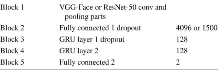
Table 6 shows the configuration of the CNN-RNN archi-tecture. The CNN part of this architecture was based on the convolutional and pooling layers of the CNN architectures described above (VGG-Face, or ResNet-50) that was fol-lowed by a fully connected layer. Note that in the case of scenario B.2 of Sect. 4.2.1, both the outputs of the last pool-ing layer of the CNN, as well as the 68 landmark 2-D posi-tions ( 68×2 values) were provided as inputs to this fully
connected layer. Table 6 shows the respective number of units for the GRU and the fully connected layers. We call this CNN plus RNN architecture AffWildNet and illustrate it in Fig. 9.
Table 6 The AffWildNet architecture: the fully connected 1 layer
has 4096, or 1500 hidden units, depending on whether VGG-Face or ResNet-50 is used
Block 1 VGG-Face or ResNet-50 conv and pooling parts
Block 2 Fully connected 1 dropout 4096 or 1500
Block 3 GRU layer 1 dropout 128
Block 4 GRU layer 2 128
Network evaluation has been performed by testing dif-ferent parameter values. The parameters included: the batch size and sequence length used for network parameter updat-ing, the value of the learning rate and the dropout probabil-ity value. Final selection of these parameters was similar to the CNN cases, apart from the sequence length which was selected in the range 50–200 and batch size that was selected in the range 2–10. Best results have been obtained with sequence length 80 and batch size 4. We note that all deep learning architectures have been implemented in the Tensorflow platform.
4.3 Experimental Results
In the following we present the affect recognition results obtained when applying the above derived CNN-only and CNN plus RNN architectures to the Aff-Wild database.
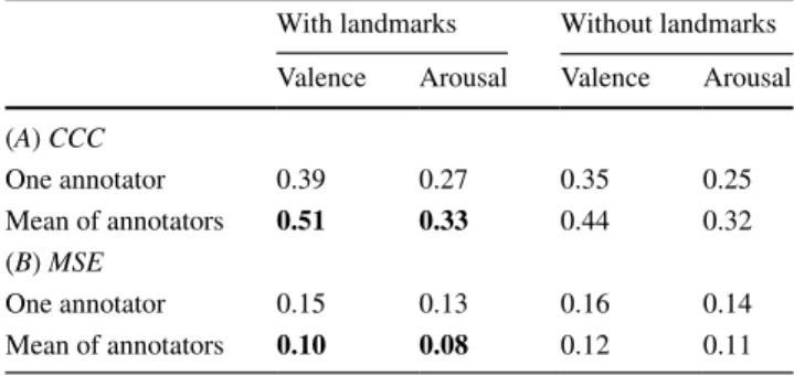
At first, we have trained the VGG-Face network using two different annotations. One, which is provided in the Aff-Wild database, is the average of the selected (as described in Sect. 3.4) annotations. The second is that of a single annota-tor (the one with the highest correlation to the landmarks). It should be mentioned that the latter is generally less smooth than the former, average, one. Hence, they are more difficult to be modeled. Then, we tested the two trained networks in two scenarios, as described in Sect. 4.2.1 case B, using/not using the 68 2-D landmark inputs.
The results are summarized in Table 7. As was expected, better results were obtained when the mean of annotations was used. Moreover, Table 7 shows that there
is a notable improvement in the performance, when we also used the 68 2-D landmark positions as input data.
Next, we examined the use of various numbers of hid-den layers and hidhid-den units per layer when training and testing the VGG-Face-GRU network. Some characteris-tic selections and their corresponding performances are shown in Table 8. It can be seen that the best results have been obtained when the RNN part of the network con-sisted of 2 layers, each of 128 hidden units.
Table 9 summarizes the CCC and MSE values obtained when applying all developed architectures described in Sects. 4.2.2 and 4.2.3, to the Aff-Wild test set. It shows the improvement in the CCC and MSE values obtained when using the AffWildNet compared to all other devel-oped architectures. This improvement clearly indicates
Fig. 9 The AffWildNet: it
consists of convolutional and pooling layers of either VGG-Face or ResNet-50 structures (denoted as CNN), followed by a fully connected layer (denoted as FC1) and two RNN layers with GRU units (V and A stand for valence and arousal respectively)
Table 7 CCC and MSE based evaluation of valence and arousal
pre-dictions provided by the VGG-Face (using the mean of annotators values, or using only one annotator values; when landmarks were or were not given as input to the network)
Best results are shown in bold
With landmarks Without landmarks Valence Arousal Valence Arousal (A) CCC One annotator 0.39 0.27 0.35 0.25 Mean of annotators 0.51 0.33 0.44 0.32 (B) MSE One annotator 0.15 0.13 0.16 0.14 Mean of annotators 0.10 0.08 0.12 0.11
the ability of the AffWildNet to better capture the dynam-ics in Aff-Wild.
In Fig. 10a, b, we qualitatively illustrate some of the obtained results by comparing a segment of the obtained valence/arousal predictions to the ground truth values, in 10000 consecutive frames of test data.
Moreover, in Fig. 11a, b, we illustrate, in the 2-D valence and arousal space, the histograms of the ground truth labels of the test set and the corresponding predic-tions of our AffWildNet.
The results shown in Table 9 and the above figures verify the excellent performance of the AffWildNet. They also show that it greatly outperformed all methods sub-mitted in the Aff-Wild Challenge.
4.4 Discussing AffWildNet’s Performance
The reasons why the AffWildNet outperformed the other methods are related to both the network design and the net-work training.
At first, the AffWildNet is a CNN-RNN network. The CNN part is based on the VGG-Face (or ResNet-50) net-work’s convolutional and pooling layers. The VGG-Face network has been pre-trained with a large dataset for face recognition (many human faces have been, therefore, used in its construction).
In our implementation, this CNN part is followed by a single FC layer. The inputs of this layer are: (a) the outputs of the last pooling layer of the CNN part; (b) the facial land-marks, which are directly passed as inputs to this FC layer. As a consequence, this layer has the role to map its two types of inputs to the same feature space, before forwarding them to the RNN part. The facial landmarks, which are provided as additional input to the network, in this way, contribute to boosting the performance of our model. The output of the fully connected layer is then passed to the RNN part.
The RNN is used in order to model the contextual infor-mation in the data, taking into account temporal variations. The RNN is composed of 2-layers, with GRU units in each layer; the first layer processes the FC layer outputs, the sec-ond layer is followed by the output layer that gives the final estimates for valence and arousal.
Table 8 Obtained CCC values for valence and arousal estimation,
when changing the number of hidden units and hidden layers in the VGG-Face-GRU architecture. A higher CCC value indicates a better performance
Best results are shown in bold
CCC 1 Hidden layer 2 Hidden layers
Hidden units Valence Arousal Valence Arousal
100 0.44 0.36 0.50 0.41
128 0.53 0.40 0.57 0.43
150 0.46 0.39 0.51 0.41
Table 9 CCC and MSE based evaluation of valence and arousal
pre-dictions provided by: (1) the CNN architecture when using three dif-ferent pre-trained networks for initialization (VGG-16, ResNet-50, VGG-Face) and (2) the VGG-Face-LSTM and AffWildNet architec-tures (2 RNN layers with 128 units each). A higher CCC and a lower MSE value indicate a better performance
Best results are shown in bold
Valence Arousal Mean value (A) CCC VGG-16 0.40 0.30 0.35 ResNet-50 0.43 0.30 0.37 VGG-Face 0.51 0.33 0.42 VGG-Face-LSTM 0.52 0.38 0.45 AffWildNet 0.57 0.43 0.50 (B) MSE VGG-16 0.13 0.11 0.12 ResNet-50 0.11 0.11 0.11 VGG-Face 0.10 0.08 0.09 VGG-Face-LSTM 0.10 0.09 0.10 AffWildNet 0.08 0.06 0.07 0 0.1 0.2 0.3 0.4 0.5 0.6 0.7 0.8 0.9 1 ·104 −0.4 −0.2 0 0.2 0.4 0.6 0.8 1 Frames V alence Annotation Predictions Labels 0 0.1 0.2 0.3 0.4 0.5 0.6 0.7 0.8 0.9 1 ·104 −0.4 −0.2 0 0.2 0.4 0.6 0.8 1 Frames Arousa lA nnotations Predictions Labels (a)Valence (b) Arousal
Fig. 10 Predictions versus Labels for a valence and b arousal over a
Part of AffWildNet’s design was the fixing of its optimal hyper-parameters (number of FC and RNN layers, number of hidden units in these layers, batch size, sequence length, dropout, learning rate). Finally, the specification of the loss function used for network training was another important issue. Our loss function was based on the CCC, as this was the main evaluation criterion of the Aff-Wild Challenge; this was not the case in the competing methods that used the usual MSE criterion in their training phases.
As far as network training is concerned, the AffWildNet has been trained as an end-to-end architecture, by jointly training its CNN and RNN parts, rather than separately train-ing the two parts.
We would also like to mention that the data augmentation that was conducted so as to achieve a more balanced dataset,
also contributed in achieving the AffWildNet a state-of-the-art performance.
5 Feature Learning from Aff‑Wild
When it comes to dimensional emotion recognition, there exists great variability between different databases, espe-cially those containing emotions in-the-wild. In particular, the annotators and the range of the annotations are dif-ferent and the labels can be either discrete or continuous. To tackle the problems caused by this variability, we take advantage of the fact that the Aff-Wild is a powerful data-base that can be exploited for learning features, which may then be used as priors for dimensional emotion recognition. In the following, we show that it can be used as prior for the RECOLA and AFEW-VA databases that are annotated for valence and arousal, just like Aff-Wild. In addition to this, we use it as a prior for categorical emotion recognition, on the EmotiW dataset, which is annotated in terms of the seven basic emotions. Experiments have been conducted on these databases yielding state-of-the-art results and thus verifying the strength of Aff-Wild for affect recognition.
5.1 Prior for Valence and Arousal Prediction
5.1.1 Experimental Results for the Aff‑Wild and RECOLA Database
In this subsection, we demonstrate the superiority of our database when it is used for pre-training a DNN. In particu-lar, we fine-tune the AffWildNet on the RECOLA and for comparison purposes we also train on RECOLA an architec-ture comprised of a ResNet-50 and a 2-layer GRU stacked on top (let us call it ResNet-GRU network). Table 10 shows the results only for the CCC score as our minimization loss was depending on this metric. It is clear that the performance on both arousal and valence of the fine-tuned model on the Aff-Wild database is much higher than the performance of the ResNet-GRU model.
To further demonstrate the benefits of our model when predicting valence and arousal, we demonstrate a histogram
Fig. 11 Histogram in the 2-D valence and arousal space of: a
annota-tions and b predictions of AffWildNet, on the test set of the Aff-Wild Challenge
Table 10 CCC based evaluation of valence and arousal predictions
provided by the fine-tuned AffWildNet and the ResNet-GRU on the RECOLA test set. A higher CCC value indicates a better performance
Best results are shown in bold
CCC
Valence Arousal
Fine-tuned AffWildNet 0.526 0.273
in the 2-D valence and arousal space of the annotations (Fig. 12a) and predictions of the fine-tuned AffWildNet (Fig. 12b) for the whole test set of RECOLA.
Finally, we also illustrate in Fig. 13a, b the network pre-diction and ground truth for one test video of RECOLA, for the valence and arousal dimensions, respectively.
5.1.2 Experimental Results for the AFEW‑VA Database
In this subsection, we focus on recognition of emotions in the AFEW-VA database, which annotation’s is somewhat different from the annotation of the Aff-Wild database. In particular, the labels of the AFEW-VA database are in the range [ −10 , +10 ], while the labels of the Aff-Wild
database are in the range [ −1 , +1 ]. To tackle this prob-lem, we scaled the range of the AFEW-VA labels to [ −1 ,
+1 ]. Moreover, differences were observed, due to the fact that the labels of the AFEW-VA are discrete, while the labels of the Aff-Wild are continuous. Figure 14 shows
the discrete valence and arousal values of the annotations in AFEW-VA database, whereas Fig. 15 shows the corre-sponding histogram in the 2-D valence and arousal space. We then performed fine-tuning of the AffWildNet to the AFEW-VA database and tested the performance of the
Fig. 12 Histogram in the 2-D valence and arousal space of a
annota-tions and b predictions for the test set of the RECOLA database
0 1,000 2,000 3,000 4,000 5,000 6,000 7,000 −1 −0.5 0 0.5 1 Frames Valence Annotations Predictions Labels 0 1,000 2,000 3,000 4,000 5,000 6,000 7,000 −1 −0.5 0 0.5 1 Frames Arousal Annotations Predictions Labels (a) Valence (b)Arousal
Fig. 13 Fine-tuned AffWildNet’s Predictions versus Labels for a
valence and b arousal for a single test video of the RECOLA database
generated network. Similarly to Kossaifi et al. (2017), we used a fivefold person-independent cross-validation strat-egy. Table 11 shows a comparison of the performance of the fine-tuned AffWildNet with the best results reported in Kossaifi et al. (2017). Those results are in terms of the Pear-son CC. It can be easily seen that the fine-tuned AffWildNet greatly outperformed the best method reported in Kossaifi et al. (2017).
For comparison purposes, we also trained a CNN network on the AFEW-VA database. This network’s architecture was based on the convolution and pooling layers of VGG-Face followed by 2 fully connected layers with 4096 and 2048 hidden units, respectively. As shown in Table 12, the per-formance of the fine-tuned AffWildNet, in terms of CCC, greatly outperformed this network as well.
All these verify that our network can be used as a pre-trained one to yield excellent results across different dimen-sional databases.
5.2 Prior for Categorical Emotion Recognition
5.2.1 Experimental Results for the EmotiW Dataset
To further show the strength of the AffWildNet, we used the AffWildNet—which is trained for dimensional emotion recognition task—in a very different problem, that of cat-egorical in-the-wild emotion recognition, focusing on the EmotiW 2017 Grand Challenge. To tackle categorical emo-tion recogniemo-tion, we modified the AffWildNet’s output layer to include 7 neurons (one for each basic emotion category) and performed fine-tuning on the AFEW 5.0 dataset.
In the presented experiments, we compare the fine-tuned AffWildNet’s performance with that of other state-of-the-art CNN and CNN-RNN networks; the CNN part of which is based on the ResNet 50, VGG-16 and VGG-Face architec-tures, trained on the same AFEW 5.0 dataset. The accuracies of all networks on the validation set of the EmotiW 2017 Grand Challenge are shown in Table 13. A higher accuracy value indicates better performance for the model. We can
Fig. 15 Histogram in the 2-D valence and arousal space of
annota-tions of the AFEW-VA database
Table 11 Pearson Correlation Coefficient (Pearson CC) based
evalu-ation of valence and arousal predictions provided by the best archi-tecture in Kossaifi et al. (2017) versus our AffWildNet fine-tuned on the AFEW-VA. A higher Pearson CC value indicates a better perfor-mance
Best results are shown in bold
Group Pearson CC
Valence Arousal
Best of Kossaifi et al. (2017) 0.407 0.45
Fine-tuned AffWildNet 0.514 0.575
Table 12 CCC based evaluation
of valence and arousal predictions provided by the CNN architecture based on VGG-Face and the fine-tuned AffWildNet on the AFEW-VA training set. A higher CCC value indicate a better performance
Best results are shown in bold CCC AFEW-VA Valence Arousal Only CNN 0.44 0.474 Fine-tuned AffWild-Net 0.515 0.556
Table 13 Accuracies on the
EmotiW validation set obtained by different CNN and CNN-RNN architectures versus the fine-tuned AffWildNet. A higher accuracy value indicates better performance
Best results are shown in bold Architectures Accuracy
Neutral Anger Disgust Fear Happy Sad Surprise Total
VGG-16 0.327 0.424 0.102 0.093 0.476 0.138 0.133 0.263 VGG-16 + RNN 0.431 0.559 0.026 0.07 0.444 0.259 0.044 0.293 ResNet 0.31 0.153 0.077 0.023 0.534 0.207 0.067 0.211 ResNet + RNN 0.431 0.237 0.077 0.07 0.587 0.155 0.089 0.261 VGG-Face + RNN 0.552 0.593 0.026 0.047 0.794 0.259 0.111 0.384 Fine-tuned AffWildNet 0.569 0.627 0.051 0.023 0.746 0.709 0.111 0.454
easily see that the AffWildNet outperforms all those other networks in terms of total accuracy.
We should note that:
(i) The AffWildNet was trained to classify only video frames (and not audio) and then video classification based on frame aggregation was performed
(ii) The cropped faces provided by the challenge were only used (and not our own detection and/or normali-zation procedure)
(iii) No data-augmentation, post-processing of the results or ensemble methodology have been conducted. It should also be mentioned that the fine-tuned AffWildNet’s performance, in terms of total accuracy, is:
(i) Much higher than the baseline total accuracy of 0.3881 reported in Dhall et al. (2017).
(ii) Better than all vanilla architectures’ performances that were reported by the three winning methods in the audio–video emotion recognition EmotiW 2017 Grand Challenge (Hu et al. 2017; Knyazev et al.
2017; Vielzeuf et al. 2017).
(iii) Comparable and better in some cases than the rest of the results obtained by the three winning methods (Hu et al. 2017; Knyazev et al. 2017; Vielzeuf et al.
2017).
The above are shown in Table 14. Those results verify that the AffWildNet can be appropriately fine-tuned and suc-cessfully used for dimensional, as well as for categorical emotion recognition.
6 Conclusions and Future Work
Deep learning and deep neural networks have been suc-cessfully used in the past years for facial expression and emotion recognition based on still image and video frame analysis. Recent research focuses on in-the-wild facial anal-ysis and refers either to categorical emotion recognition, targeting recognition of the seven basic emotion catego-ries, or to dimensional emotion recognition, analyzing the valence–arousal (V–A) representation space.
In this paper, we introduce Aff-Wild, a new, large in-the-wild database that consists of 298 videos of 200 subjects, with a total length of more than 30 h. We also present the Aff-Wild Challenge that was organized on Aff-Wild. We report the results of the challenge, and the pitfalls and chal-lenges in terms of predicting valence and arousal in-the-wild. Furthermore, we design a deep convolutional and recurrent neural architecture and perform extensive experi-mentation with the Aff-Wild database. We show that the generated AffWildNet provides the best performance for valence and arousal estimation on the Aff-Wild dataset, both in terms of the Concordance Correlation Coefficient and the Mean Squared Error criteria, when compared with other deep learning networks trained on the same database.
Subsequently, we then demonstrate that the AffWildNet and Aff-Wild database constitute tools that can be used for facial expression and emotion recognition on other data-sets. Using appropriate fine-tuning and retraining meth-odologies, we show that best results can be obtained by applying the AffWildNet to other dimensional databases, including the RECOLA and the AFEW-VA ones and by
Table 14 Overall accuracies
of the best architectures of the three winning methods of the EmotiW 2017 Grand Challenge reported on the validation set versus our fine-tuned AffWildNet. A higher accuracy value indicates better performance
Best results are shown in bold
Group Architecture Total accuracy
Original After fine-tuning
on FER2013 Data augmen-tation
Hu et al. (2017) DenseNet-121 0.414 – –
HoloNet 0.41
ResNet-50 0.418
Knyazev et al. (2017) VGG-Face 0.379 0.483 –
FR-Net-A 0.337 0.446 –
FR-Net-B 0.334 0.488 –
FR-Net-C 0.376 0.452 –
LSTM + FR-NET-B – 0.465 0.504
Vielzeuf et al. (2017) Weighted C3D (no overlap) – – 0.421
LSTM C3D (no overlap) 0.432
VGG-Face 0.414
VGG-LSTM 1 layer 0.486
comparing the obtained performances with other state-of-the-art pre-trained and fine-tuned networks.
Furthermore, we observe that fine-tuning on the AffWildNet can produce state-of-the-art performance, not only for dimensional, but also for categorical emo-tion recogniemo-tion. We use this approach to tackle the facial expression and emotion recognition parts of the EmotiW 2017 Grand Challenge, referring to recognition of the seven basic emotion categories, finding that we produce comparable or better results to the winners of this contest.
It should be stressed that it is the first time, to the best of our knowledge, that the same deep architecture can be used for both types of dimensional and categorical emotion anal-ysis. To achieve this, the AffWildNet has been effectively trained with the largest existing, in-the-wild, database for continuous valence–arousal recognition (regression analy-sis problem) and then used for tackling the discrete seven basic emotion recognition (classification) problem.
The proposed procedure for fine-tuning the AffWildNet can be applied to further extend its use in the analysis of other new visual emotion recognition datasets. This includes our current work on extending the Aff-Wild with new in-the-wild audiovisual information, as well as using it as a means for unifying different approaches to facial expression and emotion recognition. These approaches contain dimensional emotion representations, basic and compound emotion categories, facial action unit repre-sentations, as well as specific emotion categories met in different contexts, such as negative emotions, emotions in games, in social groups and other human machine (or robot) interactions.
Acknowledgements The work of Stefanos Zafeiriou has been
par-tially funded by the FiDiPro Program of Tekes with Project Number
1849/31/2015. The work of Dimitris Kollias was funded by a Teaching Fellowship of Imperial College London. The support of the EPSRC Centre for Doctoral Training in High Performance Embedded and Distributed Systems (HiPEDS, Grant Reference EP/L016796/1) is gratefully acknowledged. We also thank the NVIDIA Corporation for donating a Titan X GPU. We would like also to acknowledge the con-tribution of the Youtube users that gave us the permission to use their videos (especially Zalzar and Eddie from The1stTake). We wish to thank Dr A Dhall for providing us with the data of the Emotiw 2017 Grand Challenge. Additionally, we would like to thank the reviewers for their valuable comments that helped us to improve this paper.
Open Access This article is distributed under the terms of the
Crea-tive Commons Attribution 4.0 International License (http://creat iveco mmons .org/licen ses/by/4.0/), which permits unrestricted use, distribu-tion, and reproduction in any medium, provided you give appropriate credit to the original author(s) and the source, provide a link to the Creative Commons license, and indicate if changes were made.
A Appendix
A.1 Baseline: CNN‑M
The exact structure of the network is shown in Table 15. In total, it consists of 5 convolutional, batch normalization and pooling layers and 2 fully connected (FC) ones. For each convolutional layer the parameters are the filter and the stride, in the form of (filter height, filter width, input chan-nels , output chanchan-nels/feature maps) and (1, stride height, stride width , 1), respectively, and for the max pooling layer the parameters are the ksize and stride, in the form of (pool-ing height, pool(pool-ing width, input channels, output channels) and (1, stride height, stride width , 1), respectively. We fol-low the TensorFfol-low’s platform notation for the values of all those parameters. Note that the activation function in the
Table 15 Baseline architecture
based on CNN-M, showing the values of the parameters of the convolutional and pooling layers and the number of hidden units in the fully connected layers. We follow the TensorFlow’s platform notation for the values of all those parameters
Layer Filter Ksize Stride Padding No. of units
conv 1 [7, 7, 3, 96] [1, 2, 2, 1] ‘VALID’
batch norm
max pooling [1, 3, 3, 1] [1, 2, 2, 1] ‘VALID’
conv 2 [5, 5, 96, 256] [1, 2, 2, 1] ‘SAME’
batch norm
max pooling [1, 3, 3, 1] [1, 2, 2, 1] ‘SAME’
conv 3 [3, 3, 256, 512] [1, 1, 1, 1] ‘SAME’ batch norm conv 4 [3, 3, 512, 512] [1, 1, 1, 1] ‘SAME’ batch norm conv 5 [3, 3, 512, 512] [1, 1, 1, 1] ‘SAME’ batch norm
max pooling [1, 2, 2, 1] [1, 2, 2, 1] ‘SAME’
Fully connected 1 4096