Multi-Modal Learning For Adaptive Scene Understanding

(1)

Multi-Modal Learning For Adaptive

Scene Understanding

Charika Sanjeewani De Alvis Weerasiriwardhane

A thesis submitted in fulfillment of the requirements for the degree of

Doctor of Philosophy

Faculty of Engineering and Information Technologies University of Sydney

(2)

Declaration

I hereby declare that this submission is my own work and that, to the best of my knowledge and belief, it contains no material previously published or written by another person nor material which to a substantial extent has been accepted for the award of any other degree or diploma of the University or other institute of higher learning, except where due acknowledgement has been made in the text.

Charika Sanjeewani De Alvis Weerasiriwardhane

(3)

Abstract

Charika De Alvis Doctor of Philosophy

University of Sydney January 2017

Multi-Modal Learning For

Adaptive Scene Understanding

Modern robotics systems typically possess sensors of different modalities such as colour cameras, inertial measurement units, and 3D laser scanners to per-ceive their environment. While there are undeniable benefits to combine sensors of different modalities the process tends to be complicated. Segmenting scenes observed by the robot into a discrete set of classes is a central requirement for autonomy as understanding the scene is the first step to reason about future situations. Equally, when a robot navigates through an unknown environment, it is often necessary to adjust the parameters of the scene segmentation model online to maintain the same level of accuracy in changing situations. This the-sis explores efficient means of adaptive semantic scene segmentation in an online setting with the use of multiple sensor modalities

In computer vision many successful methods for scene segmentation are based on conditional random fields (CRF) where the maximum a posteriori (MAP) solu-tion to the segmentasolu-tion problem can be obtained by efficient inference. CRF encodes contextual information and longer-range relationships during the predic-tion process. Further, parameters learning of CRFs is a also widely studied area This thesis offers three main contributions.

First, we devise a novel CRF inference method for scene segmentation that in-corporates global constraints, enforcing particular sets of nodes to be assigned the same class label. To do this efficiently, the CRF is formulated as a relaxed quadratic program whose MAP solution is found using a gradient-based opti-misation approach. These global constraints are useful, since they can encode "a priori" information about the final labeling. This new formulation also re-duces the dimensionality of the original image-labeling problem, which result in a decrease of the computational time. The proposed globally constrained CRF is employed in an urban street scene understanding task. Camera data is used for the CRF based semantic segmentation while global constraints are derived from 3D laser point clouds. Experimental results demonstrate the improvement achieved with global constraints. Comparisons with higher order potential CRF show the benefits of the proposed method.

Second, an approach to learn CRF parameters without the need for manually la-belled training data is proposed. Parameter learning is of high importance when

(4)

data is unknown. The model parameters are estimated by optimising a novel loss function using self supervised reference labels. These reference labels are obtained purely based on the information from camera and laser, in a self-training man-ner with minimum amount of human supervision. Sensor data is pre-processed using methods such as convolutional nets, discriminant analysis, and Euclidean distance based clustering to extract reference labels

Third, an approach that can conduct the parameter optimisation while increasing the model robustness to non-stationary data distributions in the long trajectories of the robot is proposed. We adopted stochastic gradient descent to achieve this goal by using a learning rate that can appropriately grow or diminish to gain adaptability to changes in the data distribution. We demonstrate experimental results on KITTI dataset for long real world image sequences.

(5)

Acknowledgments

I would like to express special gratitude to my supervisor Fabio Ramos for the strong support and guidance you have provided to conduct quality research. The freedom to explore and timely feedback were incredibly helpful to make this journey a success. I would also thank NICTA for the financial support during the period my candidature. Furthermore I would also like to thank Lionel Ott for the support and collaborations throughout in the development of the thesis. My special thanks to all of my colleagues in Fabio's group for the interesting chats and the shared ideas. I would finally like to express my appreciation towards my loving husband, and to my mother for the confidence you built in me.

(6)

Nomenclature

General

P(A) Probability of event A

P(A|B) Probability of event A given event B

K−1 _{Matrix inversion}

KT Matrix transpose

Kij Element of matrix K at row i and columnj

L Set of Labels

n Number of labels

x Multidimensional observed variable

D Dimension of x

xi ith element of vector x

||x|| L2 _{norm of vector} _x

y Multidimensional target variable

θ Model parameters

θ∗ Optimal parameter values

g(x) Function over x

Classificication

ai Training data samples in class i

ki Number of data samples in ai

¯

xi Average of the data samples in ai

Γ1 Intra class covariance matrix

Γ2 Inter class covariance matrix

Φ Linear transformation matrix

Conditional Random Fields

G Undirected graph

V Set of vertices

E Set of edges

C Set of cliques in a graph

m Number of nodes in the graph

Ni Neighbours of node i

(7)

yi Trarget variable correspond to node i.

ψi(yi) Unary potental of node i

ψij(yi, yj) Pairwise potental between nodes i and j

E(y|θ) Energy of the model given parameters

Ω Training set

N Number of training samples

K Number of parameters

L(θ|Ω) Likelihood of θ given data

l(θ|Ω) Log likelihood function E(f(x)) Expected value of f(x)

C Global constraints

Convex Relaxation

I(yi), I(yi, yj) Indicator variables of label assignment

H Edge potential matrix

Equality Constrained Quadratic Programming

Q Negative edge potential matrix

A Equality constraints matrix

e Number of equality constraints

λ Lagrange multiplier vector

null(A) Null space of matrix A

Z Basis for the null space

˜

Q Reduced hessian matrix

Belief Propagation

mi→j Message from i toj

Bi Belief in node i

Ni/j Neighbourhood of i except j

Optimisation

w Image frame index

(8)

EN Empirical risk

η Global learning rate

t Iteration index

θt Value of parameter at tth iteration

γ Global learning rate for SGD

5f(x) Gradient of f at x

α, λ Loss function parameters

z Ground truth labels

B Mini batch size

3D Point Cloud Processing

M Horizontal plane model

h0 Number of points required to learn parameters of M

Pn Observed data distribution

T Number of iterations

Si Set of points fit with the model

¯

Si Consensus set of Si

ν Probability of outlier occurrence

, γ Threshold values

R kd tree formulation of point cloud

QR Queue of points

CL List of clusters

dn Radius of point neighbourhood

du Upper bound

Ci Cluster i

Visual Features and Metrics

l, a, b LAB color metrics

x, y Image pixel location coordinates

ω Data sample

Dxy Distance in x−y coordinate frame

Dlab Distance in LAB color space

Dr Distance between cluster centers

DB Bhattacharyya Distance

DE Euclidean Distance

M Superpixel count

(9)

m Pixel count

ξ Compactness indicator

NB Number of bins in a histogram

Abbreviations

CRF Conditional Random Field

FCN Fully Convolutional Net

GD Gradient descent

GPS Global positioning system

HOG Histogram of oriented gradients

HOP Higher order potentials

ICM Iterative conditional modes

ILP Integer linear programming

LBP Loopy bilief propagation

LDA Linear discriminant analysis

ML Maximum Likelihood

MAP Maximum a Posteriori

MCMC Markov chain Monte Carlo

pLDA Pseudo linear discriminant analysis

QP Quadratic programming

RANSAC Random sample consensus

SGD Stochastic gradient descent

SIFT Scale-Invariant Feature Transform

SLIC Simple linear iterative clustering

UGM Undirected graphical models

(10)

(11)

List of Figures

1.1 Semantically Segmented Image . . . 2

1.2 Google Self Driving Vehicle . . . 2

1.3 Example of a CRF model . . . 3

1.4 KITTI autonomous driving platform . . . 4

1.5 Point clusters generated from a 3D Velodyne point cloud . . . 5

2.1 Image intensity histograms . . . 35

2.2 HOG features . . . 36

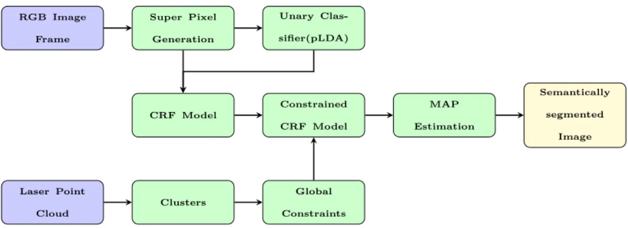
3.1 Block diagram of CQP model . . . 46

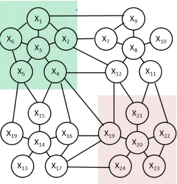
3.2 Example of a CRF graph . . . 50

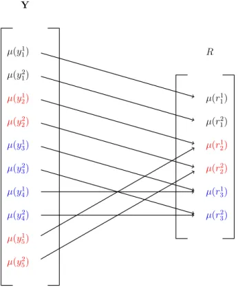
3.3 Mapping from Y to R . . . 53

3.4 Camera and laser data pre-processing techniques . . . 59

3.5 Visual data based scene segmentation results . . . 60

3.6 Visual data based scene segmentation quantitative analysis plots . 61 3.7 Examples of scenes segmented using CQP . . . 63

3.8 Laser Based Hard Constraints . . . 64

3.9 Gradient based optimisation process . . . 65

3.10 Value of the objective over each iteration . . . 66

3.11 Experiments on Ford Vision and Lidar dataset . . . 68

3.12 Runtime comparison . . . 69

4.1 Block diagram the adaptive learning model . . . 73

4.2 Accuracy plots for adaptive learning model . . . 85

4.3 Example images for qualitative analysis . . . 86

4.4 Reference labels . . . 86

4.6 Relative accuracy plots . . . 87

4.5 Label consistency reference . . . 87

4.7 Class based accuracy plots . . . 89

4.8 Analysis of robustness to changes in input data . . . 90

4.9 Performance analysis of optimised parameters . . . 91

(15)

List of Tables

3.1 Visual features . . . 57 3.2 Overall quantitative analysis of scene segmentation models . . . . 65 3.3 Class wise quantitative analysis of scene segmentation models . . 66 3.4 Quantitative evaluation on the Ford vision and lidar datase . . . . 67

4.1 Loss function parameters . . . 83 4.2 Quantitative comparison of CQP and online CQP . . . 88 4.3 Classwise accuracy of online CQP . . . 88

(16)

List of Algorithms

1 Loopy Belief Propagation for Pairwise CRF . . . 18

2 SLIC Super pixels . . . 32

3 RANSAC . . . 38

4 Euclidean Cluster Extraction . . . 39

5 Globally Constrained CRF . . . 55

(17)

Chapter 1 Introduction

1.1 Motivation

Intelligent autonomous systems are becoming increasingly popular in society. Driver assistance, robotic navigation and environmental exploration all include a level of autonomy. Autonomous driving is highly beneficial because it con-tributes to reducing road accidents, creating orderly traffic flow, optimising fuel consumption and providing mobility for the elderly and people with disabili-ties. Under autonomous driving, there are many areas of active research, such as road, vehicle, traffic sign and pedestrian detection and understanding. There-fore, it is necessary to establish a semantic and geometrical understanding of the changing environment surrounding the vehicle. For this purpose, identifying the precise class boundaries is critical. Object or class recognition is usually achieved through labelling every pixel of the image with a chosen class or object label. Figure 1.1 shows a semantically segmented street scene to 12 distinct classes. Google’s self-driving car is arguably a successful attempt to fully automate the task of autonomous driving. However, complete autonomy is still infeasible due to the nonlinearities in real world applications. Figure 1.2 is an image of the Google self-driving car with a 360◦ Velodyne scanner.

Scene understanding is commonly studied in the context of autonomous driving and comes with major challenges. A successful scene understanding algorithm should have the capability to accommodate rich contextual information in the process of segmenting the image over accurate class boundaries and subsequently assigning class labels to each segment. For image labelling problems, Conditional Random Fields (CRF) are commonly used because they can integrate different levels of contextual information. CRF has unary potentials that can capture low-level cues derived from local texture, colour and location of the pixels and pairwise potentials that can assist in smoothing label predictions. Figure 1.3 de-picts a simple CRF model built over image patches. Higher-level cues such as label consistency in regions, object co-occurrence statistics and shape informa-tion can be incorporated in the CRF model through higher order potentials or hierarchical connectivity.

(18)

Figure 1.1: Illustration of semantic segmentation of an image. Pixels correspond to different object classes are individually. From: http://mi.eng.cam.ac.uk/projects/segnet/.

Figure 1.2: Google self driving car(courtesy NASA/JPL-Caltech).

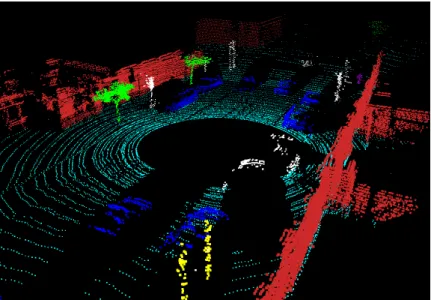
Higher-level cues that contain longer-range information such as label consis-tency over image regions are typically derived using unsupervised image seg-mentation methods such as clustering. Clustering algorithms group similar data points within the given data. The similarity of the data in a group provides information about label consistency. The importance of clustering is that it re-quires minimum human supervision and can be modelled to adapt to changing environments. Furthermore, clustering algorithms do not require assumptions on the input data since they group data into separate clusters based on the dis-similarity metrics. Moreover, clustering is an attractive technique to reduce the dimensionality of the data and also especially suitable for processing sparse data. For sparse 3D laser point cloud processing, clustering techniques are efficiently implemented [90]. Figure 1.5 shows clusters generated from a 3D point cloud where each cluster correspond to an object or a part of an object. However, the accuracy of the final solution of CRF based semantic scene segmentation models is limited by the accuracy of the associated unsupervised methods.

For accurate scene labelling output it is necessary to learn the CRF parameters corresponding to the input data distribution, which requires inference over the CRF model.

(19)

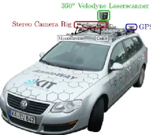
Figure 1.3: Autonomous driving platform Annieway with multiple sensor modalities (courtesy Annieway /KITTI).

The scene segmentation problem typically formulated by grid shaped CRF and it results in complicated dependencies in the model, further it also involves multi-ple classes/states, essentially rendering the inference problem intractable. Under these circumstances, accurate CRF parameter learning can be a challenging task. Typically, CRFs are used to encode visual information, such as colour and tex-ture for scene classification. However, it is evident that combination of multiple modalities can be beneficial, i.e. using depth information in addition to visual data can increase the robustness to changes in illumination and texture; and as a result, we see that contemporary robots are comprised of multiple sensors such as optical cameras, Velodynes, sonars, thermal cameras and flash lidars. Figure 1.4 shows autonomous driving platform of KITTI vision benchmark suite with mul-tiple modalities mounted on it. Laser-based depth information is commonly used with visual information to CRF modelling. The tendency to use multiple modal-ities has drawn more attention towards efficient sensor fusion techniques.

Another consideration is that the location and orientation of each sensor may vary from each other. As a result, the visibility of an object might change from sensor to sensor due to occlusions. Laser sensors usually can perceive objects in a shorter range, while cameras can capture objects much further. This shows that, some sensors are capable of recognising particular object classes better than others. Therefore, efficient sensor fusion requires representing all different sensor inputs in one single domain. This is a complex task, and so substantial research is being conducted on fusing sensors to get the maximum use of input data. Apart from that the scene segmentation model should have the flexibility to fuse information from any new sensor input introduced to the system.

Semantic scene segmentation directly links with autonomous driving. Scene labelling models are learnt on training datasets, eventhough the model has to operate on newly encountered data. In scenarios where the autonomous vehicle

(20)

Figure 1.4: Part of a conditional random field built over an image patches. Demon-strates characterization of contextual information. From: http://spark-university.s3.amazonaws.com/stanford-pgm/slides/2.4.1-Repn-MNs-pairwise.pdf.

navigates in unknown changing environments, maintaining a high level of accu-racy of image labelling is very challenging. One option is to use large datasets of labelled samples to train the model, since it should improve the generalisa-tion properties. But this involves large amounts of human supervision, increases computational complexity and time consumption. In other words, autonomy be-comes an unrealistic goal. Additionally, it is impractical to obtain labelled data when navigating in unknown environments. There can be an infinite number of different routes, changing weather, lighting conditions, traffic conditions and so on. Therefore it is essential to generate means of establishing adaptability in unexpected scenarios.

When developing adaptive scene segmentation models for autonomous driving, online learning plays a significant role. As new data instances are observed, CRF model parameters can be updated in an online setting. Batch optimisers that update parameter with the use of gradient and Hessian computations accumu-lated over the complete training set are a popular choice for parameter learning. However, in autonomous driving, the relevant data stream is continuous. As the vehicle moves, new data flows in which makes it hard to define a fixed-length batch of data. Furthermore, using batch optimizing on past data also can be infeasible due to the sheer amount of information. Consequently, stochastic gradient-based methods that update the model parameters based on the gradient over a sin-gle data instance are commonly utilised in place of batch optimisers. Stochastic methods scale appropriately with advanced computing resources and are also re-silient to the inaccuracies that occur when approximating the gradients.

(21)

Figure 1.5: Point clusters generated from a 3D Velodyne point cloud conrrespond to individual objects. From: http://www.roboticsproceedings.org/rss05/p22.pdf.

Additionally, there is evidence showing that models trained using stochastic gra-dient descent(SGD) tend to have lower generalisation errors compared to batch learning methods.

However, using SGD in an online setting comes with challenges. Selecting an optimum learning rate for SGD methods can be complicated since larger learn-ing rates result in divergence from the optimum parameter values and smaller learning rates can make the learning process extremely slow. Slow adaptation is unsuitable for real-time operation, especially when navigating in an urban en-vironment, where it is essential to understand the environment in a real-time manner. Hence we need a way to optimise the parameters of the CRF efficiently and accurately. It has been shown in the literature that decreasing learning rates guarantee the convergence of SGD, and so diminishing learning rate is commonly used in practice. However, for non-stationary data distributions, the optimiser might become trapped in a local minimum as the the learning rate becomes in-finitesimal, and so new information cannot be learned. Even fixed learning rates cannot address this issue, therefore it is important to have an adaptable learning rate that can increase or decrease according to changes in the data distribution.

1.2 Problem Statement

The thesis addresses the following critical issues in autonomous navigation. Ini-tially, it focuses developing a convenient way of including “a priori ”knowledge about correct labelling to the scene segmentation model in the optimisation pro-cess, because this type of additional information is readily available and can be

(22)

is commonly obtained by combining information from different modalities. Sec-ondly, we consider the problem in the context of typical autonomous platforms that consist of cameras and laser sensors as the primary sensors of interest. In this scenario, using laser-based information as additional knowledge to image based scene segmentation models has to be analysed further to increase the efficiency. Thirdly, this thesis addresses the issues involve with scene segmentation during long-term navigation where the main problem concerns modelling adaptability in changing environments. The core of the thesis thus demonstrates a method that can adapt to the variations in the perceived environment through an efficient pa-rameter learning method. Furthermore, the computational cost of the semantic segmentation of an image frame is minimised, thus facilitating real-time oper-ation. Finally, we explore means of eliminating the need for manually labelled data during the learning process.

1.3 Contributions

The major contributions of this thesis are as follows:

1. A novel CRF formulation using global constraints capable of en-forcing label consistency in a semantic scene segmentation model for autonomous driving. An application of the proposed method is demonstrated for urban street scene segmentation using cam-era and laser sensor data gathered by real robotic platforms. CRF can be used to model the image labeling problem. Label prediction is formulated as the maximum a posteriori (MAP) estimation problem of CRF. Quadratic programming (QP) formulation is one of the most efficient means of solving the CRF inference problem. We propose an inference method to include "a priori" information about label consistency in the form of constraints. A side effect of the use of these constraints is a large reduction of the problem’s dimensionality which facilitate real-time opera-tion. Experiments shows how constrained CRF is used to efficiently fuse camera and laser sensors efficiently. The CRF model is formulated based on visual features obtained from camera images, and global constraints that enforce label consistency are extracted from the laser point cloud. This approach enhances the model’s resilience to changes in lighting conditions and occlusions.

2. Developing an approach for CRF parameters learning eliminating the need for manually labelled training data.

(23)

CRF parameters estimation is essential to efficiently combine the different cues associated with the model since it enriches the adaptability of the model. Parameter learning is formulated on the optimisation of a loss func-tion.

Our approach derives the reference labels necessary for the loss computa-tion in a self supervised manner based on the outputs from a discriminant analysis classifier and a fully convolutional network combined with laser point based segments corresponding to objects in the image. This approach minimises the human supervision in learning by providing means for the model to automatically learn from unseen instances.

3. A stochastic gradient based method to update CRF parameters while making the model robust to non-stationary data in long-term navigation.

The Semantic scene segmentation model is extended to an online learning algorithm, where the model updates its parameters to predict image labels more accurately over time. Since the input data stream is large and un-known, stochastic gradient descent is used to optimise the loss as new data is received. The learning rate is continuously adjusted, both decreasing over time to allow the model to reach an optimum point and increasing when necessary to leap out of a local minima. The proposed model has the ca-pability to maintain or improve the accuracy of its initial estimates as the perceiving environment changes.

1.4 Thesis Outline

This section summarises the content of the thesis. The goal is to develop an efficient framework for scene understanding to assist with autonomous driving. Accurate scene understanding is expected to be achieved through the addition of "a priori" knowledge in the form of global constraints, while getting the maximum use of the input data from multiple modalities. The model is designed to adpat to the changes in the environment when navigating in urban environments.

Chapter 2: Theoretical Background

This chapter describes the fundamental theories and techniques necessary to de-velop the original contributions of the thesis. It starts with an introduction to supervised learning (section 2.1) and then details an specific classification algo-rithm, discriminant analysis. Afterwards, the theory of conditional random fields (CRFs) is explained (section 2.2). Under this section, the formulation of CRF,

(24)

general inference, inference using programming relaxations and parameter learn-ing of CRF are described. Sections 2.3 and 2.4 detail the batch gradient descent and stochastic gradient descent methods, which are commonly used in parame-ter learning. Finally, section 2.5 presents information on sensor data processing, focusing specifically on camera images and laser point clouds.

Chapter 3: Urban Scene Segmentation with Laser-Constrained CRFs This chapter discusses the first contribution of the thesis related to developing a reliable scene understanding framework. Section 3.1 consists of the introduc-tion and related work of the proposed model. Secintroduc-tion 3.2 introduces the CRF based semantic scene segmentation model, that incorporates camera-based vi-sual information and laser based global constraints. In section 3.3, inference in the proposed CRF model is illustrated. This section expands on how quadratic programming formulation can be used to characterise the image labeling prob-lem with global constraints. Finally, section 3.4 demonstrates the benefit of the proposed semantic segmentation model over other state of the art methods that only exploit visual information. Furthermore, it also showcases the advantage of having laser-based hard constraints over methods using soft constraints. Experi-mental results are presented for two real-world data sets.

Chapter 4: Online Learning for Scene Segmentation With Laser Constrained CRFs

This chapter focuses on the second and third contributions of this thesis, which are developed by extending the proposed scene segmentation model to an online adaptive model. Section 4.1 provides the introduction to the framework and dis-cusses related work. Section 4.2 describes the process of extending the constrained QP problem in to an adaptive model by parameter learning using self supervised reference labels. It details that how stochastic gradient descent methods can be used to learn the parameters efficiently. Lastly, section 4.4 demonstrates the en-hancement in quality achieved for individual object classification with adaptive learning. It also showcases the robustness of the scene segmentation model over long image sequences to simulate real-world driving. Finally, it illustrates the adaptability of the model to abrupt changes of input data distribution

Chapter 5: Conclusion and Future Work

Chapter 5 summarises the contributions of the thesis and draw conclusions based on the proposed methods. This chapter concludes by suggesting directions for future research on semantic scene segmentation based on the proposed framework.

(25)

Chapter 2 Background

This chapter presents the theoretical background necessary to understand the thesis. In Section 2.1 we introduce supervised learning techniques. We discuss classification algorithm, Discriminant Analysis, which we have utilised in our work to obtain the basic predictions on image labels.

Section 2.2 provides a description of Conditional Random Fields, which is also a sophisticated method for enhancing the quality of image classification considering the longer-range contextual information. Here we discuss about the inference in CRF and possible approaches to solve the inference problem. We majorly focus on the Quadratic Programming that can be efficiently applied in image classification. Further this section provides information on parameter estimation of CRF models.

The approaches used for optimisation in machine learning are described in the Section 2.3 and 2.4. Section 2.3 introduces gradient descent algorithm in general. Our research involves with developing an adaptive model requiring parameter optimisation. Stochastic gradient decent, which is detailed in section 2.4, is im-plemented for optimising the parameters for our CRF model to conduct image segmentation. Since our problem operates in an online setting the problem is large scale and stochastic gradient methods are more attractive.

The Section 2.5 presents information on sensor data processing. This section contains two portions. The first part explains image data processing. The sec-ond part is focused on 3-D point cloud processing. We provide details on super pixels generation and feature extraction. Laser point cloud based 3D information plays a major role in our image classification framework. We describe 3D point cloud processing methods such as Euclidean cluster extraction and ground plane removal methods.

2.1 Supervised Learning

Supervised learning is a major branch in machine learning. Consider target vari-ables y and observed variables x where y = g(x). In supervised learning, the main task is learning the function g parameterised by a set of parameters θ given

(26)

training set. Learning is conducted using a training set of input and output sam-ples Ω ={(xi, yi)}Ni=1 assumed to be independent and identically distributed. N

refers to the number of training samples. xi has D number of dimensions, where

each dimension links to a feature or a attribute. Features are extracted from an image, sentence, electronic signal or voice recording. In the case where yi is a

real valued scalar the prediction problem is referred as regression. Normally the output yi is considered to be a categorical or nominal variable and can be

assigned with a value from the setL={1, ..,n}wheren is the number of classes. This type of a problem is known as classification. Murphy et al. [75] offers a more extensive theoretical description of the properties and the applications of supervised learning.

2.1.1 Classification

In classification problems, when n = 2 then the problem reduces in to a binary classification whenn >2 it is a multiclass classification. Through machine learn-ing the classifier function g is obtained. Subsequently, the learnt function can be used to predict the label of newly observed data. However, it is important that function g generalises well to unseen data. There are several algorithms used for classification such as Support vector machines [20], Decision Trees [84] and Neu-ral Networks [3] . In the next section we explain the theory behind discriminant analysis utilised in extracting labels for the image pixels in later chapters.

Linear Discriminant Analysis

Linear discriminant analysis (LDA) linearly combines features to distinguish be-tween object classes. It can be directly used as a linear classifier or for dimension-ality reduction. This is a popular technique for pattern classification mainly due to the ease of computation since it has closed form solutions. It also provides de-cent class separability and can be used for multiclass problems intrinsically. This classifier has demonstrated good performance in practice. Additionally LDA does not require learning of hyper parameters. In our work, we use LDA to classify image patches. Li et al. [64] proposed the first LDA model to map multivariate input variables to univariate output variables. Here the model ensures that the outputs generated from each of the classes are far from each other as much as possible. Consider a training set Ω. The dimensionality D of input vectorx has to be sufficiently large to contain adequate information to conduct the classifica-tion accurately. LDA is developed based on the analysis of scatter matrix, which is a metric utilised to evaluate the covariance matrix of the multivariate normal

(27)

distribution. The corresponding scatter matrix for class i is denoted by:

χi =

X

xj∈ai

(xj−x¯i)(xj −x¯i)T, (2.1)

where the number of classes is denoted byn. ai referred to input data samples of

ithclass. ¯xireferred to the mean of the example input instances that has the label

of the ith class. Fisher et al. [114] introduce a discriminative feature transform using intra-class and inter class co-variance matrices denoted by Γ1 (Eq. (2.2))

and Γ2 (Eq. (2.3)) respectively,

Γ1 = n X i=1 χi, (2.2) Γ2 = n X i=1 ki(¯xi−x¯)(¯xi−x¯)T, (2.3a) ¯ x=1 N n X i=1 kix¯i. (2.3b)

Herekirefers to the number of sample inputs belong to the classi. N denotes the

total number of samples. There are important characteristics of the matrix T = Γ−₁1Γ2 so it can convey information on class compactness and class separation. T

provides a discriminative feature transform through the eigenvectors related to the largest eigenvalues. According to Fishers criterion [114] a linear transformation Φ can be defined by maximising the Rayleigh coefficient indicated below,

Rayleigh coefficient = |Φ T_Γ 2Φ| |ΦT_Γ 1Φ| . (2.4)

This linear transformation matrix can be utilised as a distance measure (similar to Euclidean distance) to do the classification in the transformed space. The class label for some input xj is given by:

yj =i∗ where i∗ = mini∈LxjΦ−x¯iΦ. (2.5)

2.2 Conditional Random Fields

In artificial intelligence, problems such as scene understanding, natural language processing and voice recognition require computing the assignments to a sequence y given a known set of inputs x. The prediction of y can be difficult due to the complex dependencies between output variables. For instance, in image labelling

(28)

cal models [19, 81] unite the techniques in probability theory with the efficient strategies in graph theory to overcome the complexity. They can be used to represent such problems, since they can efficiently characterise the dependencies between output variables. There are several families of graphical models such as neural networks, Markov random fields [51], ising models [113], Bayesian net-works [47]and factor graphs [57] for structured prediction. Commonly, graphical models use a generative approach, which focus on modeling a joint probability distribution over input and output variables. However, CRF based approaches can result in intractable models when the dimensionality of the input is massive and there are complex dependencies between input variables. For more informa-tion on graphical models please refer to [54].

Conditional random fields (CRFs) are a variation of Markov random fields and use a discriminative approach to overcome the tedious joint probability compu-tations. CRFs characterise distributions of structured output variables that are conditioned on some observed variables. These conditional distributions can be utilised for solving sequential classification problems. Typically, discriminative models do not require modelling the input distribution and also they permit to use pre-processed inputs, which can be useful in image classification. Another advantage of CRFs in the context of image classification is that it has flexibility to incorporate global features.

A discrete random field can be defined over the graphG= (V,E) whereV and Eare the set of vertices and set of edges in the graph respectively. In this context y = {y1, y2, .., ym} is a set of random variables where each vertex is associated

with each node i. Each random variable can have a label from the label set

L = {1,2, .., n}. x represent the observed variables. Neighbours of each node i

are indicated by _Ni ={j ∈ V|(i, j) ∈ E}. Through the conditional distribution

P(y|x) the mapping from x to y is modeled. When y is conditioned on x it assumes the Markov property. That implies the conditional distribution of yi,

given its neighbours in G, is independent from the other variables which are not in the neighbourhood.

The conditional distribution for the random variable set can be indicated by:

P(y|x, θ) = 1 Z(x)

Y

c∈C

Ψc(yc|x, θ). (2.6)

Here a set of conditionally dependent random variables is defined as a clique (fully-connected sub-graphs), which is denoted by c. Set of random variables correspond to clique c is denoted by yc, where C denotes the set of all cliques

and Ψcis a non negative clique potential. Set of model parameters are indicated

(29)

function of the input x, Z(x) =X y Y c∈C Ψc(yc|x, θ). (2.7)

Generally in the cases where y is discrete, log potential is described by a linear combination of parameters,

logΨc(yc|x, θ) = θcTψc(x,yc), (2.8)

where θc ∈ R is a parameter vector. ψc indicate sufficient statistics or feature

functions learnt from the observed data. Now the log of the conditional proba-bility can be denoted by:

log(P(y|x, θ)) = X

c∈C

θ_cTψc(x,yc)−log(Z(x)). (2.9)

This formulation is known as the log-linear model. According to the theories in statistical physics, a probability distribution can be defined using the energy of the variables. This formulation is known as the gibs distribution [63],

P(y|x, θ) = 1

Z(x)exp(− X

c∈C

E(yc|θc)), (2.10)

where E(yc|θc) ≥ 0 is the energy correspond to the clique c. The conditional

distribution of the CRF can be represented from a Gibbs distribution by defining the potential as follows:

Ψc(yc|x, θ) =exp(−E(yc|θc)). (2.11)

Now the energy of the CRF model can be denoted by:

E(y|θ) =−log(P(y|x, θ))−log(Z(x)). (2.12)

CRF for Image Labelling

Image classification can be characterised as a process of assigning labels to image pixels or patches (small groups of pixels). These labels depend on the application, i.e. foreground, background or object class label. Relationships among the labels of image pixels or patches are very important. CRF models are commonly used to solve the image classification problem. Usually for image classification problems, size of maximal clique is considered as 2 by confining the model into unary and pairwise cliques.

(30)

is associated with an unary potential ψi(yi) that is defined as the log likelihood

of node iis assigned with label yi. This potential is computed based on features

extracted locally to a node, i.e. colour, texture and location. Similarly, pairwise cliques correspond to edges. Edge potentials are denoted byψij(yi, yj). Typically

these edge potentials encourage connected nodes to take the same label. In prac-tice contrast sensitive Potts models [17] are used to formulate pairwise potentials can be expressed by,

ψij(yi, yj) =      0 if (yi =yj) γ(i, j) otherwise , (2.13)

here γ(i, j) is a feature function derived on the contrast of colour, texture and location of the connecting nodes in the graph. In the general case neighbourhood Ni is stated as to connect 4 to 8 neighbouring pixels. These connections are

important since they decide the amount of contextual information is used in classification. Energy of the image classification problem can be indicated by:

E(y) = X i∈V ψi(yi) | {z } Unary Potentials + X i∈V,j∈Ni ψi,j(yi, yj) | {z } Pairwise potentials . (2.14)

Higher Order Potentials

The pairwise potential encourages smooth boundaries between different object classes. However these potentials can be highly useful but still have some draw-backs. For example, these smoothing terms are less efficient in identifying in-tricate boundaries of different object classes. In addition, the boundaries of the objects in the segmentation based on pairwise potentials can deviate from the actual boundaries due to the over smoothing. In order to address these prob-lems higher order potentials (HOPs) are introduced to the image classification problem. Higher order potentials impose soft constraints about label consistency. Thus it encourages the consistency of labelling with in image regions or segments. In this manner HOP assist to capture longer range relationships. Energy function of CRF can be modified by introducing HOPs as in Eq. (2.15), where S denotes the set of image regions/segments, on which ψa, the higher order potentials are

defined on, E(y) = X i∈V ψi(yi) + X i∈V,j∈Ni ψi,j(yi, yj) + X a∈S ψa(ya). (2.15)

(31)

2.2.1 CRF Inference

In learning the CRF model parameters and predicting the query variables, accu-rate and fast inference is a main concern. The goal of this section is to describe the main inference problems and commonly used approaches to solve them. The section mainly focus on the inference methods which would be efficiently used for image labelling problem. A more comprehensive explanation can be found in [75]. Generally two inference problems can be described for CRF.

• Marginal Distribution Computation:

The marginal distribution for a set of variables in a CRF is obtained by marginalising all the other variables to obtainP(yc|x, θ) wherecis a subset

of y. The computation involves summing out all the random variables in the conditional distribution of y that do not belong to clique c. When there are large number of variables associated with y or when variables having a higher number of states, computational complexity can increase and problem can become intractable. Selecting a simpler graph structure might reduce the computational cost.

• Maximum A Posteriori Estimation:

Considering a CRF with parameter set θ, we obtain the labelling of y correspond to inputxby picking the most likely outputyM AP _{that is stated}

as the maximum a posteriori denoted by argmax_yP(y|x, θ), yM AP = argmax y P(y|x, θ) = argmaxy 1 Z(x) Y c∈C Ψc(yc|x, θ). (2.16)

MAP estimation is widely used since it represent an optimisation problem, that can be solved by efficient algorithms. MAP inference for general graphs tend to be NP-hard in most of the cases. For those instances approximate inference is conducted. It is clear that since the normalisation function is not a function of y, it can be ignored during the optimisation process. Therefore, according to the Eq. (2.12) MAP solution also can be attained by minimising the energy function,

yM AP = arg min

y E(y). (2.17)

MAP estimation is similar to a point estimate. Hence it does not comes with any uncertainty measures.

(32)

Exact Inference

This section focuses on the exact inference in conditional random fields. For more detailed description on the algorithms mentioned here refer to [54],[50] and [80]. Usually the computational cost for the inference operations exponentially grows with the number of random variables. This causes the intractability of the exact inference in general CRF. However there are some special cases where the inference problem in CRFs can be solve in polynomial time. Variable elim-ination (VE) [54] is the simplest approach to obtain the marginal distribution or the MAP estimation of CRFs. However, this method has an exponentially growing complexity with the number of random variables. Usually VE can only be used to conduct the inference in graphs with low treewidth. Typically, when the graph has a chain or a tree structure, message-passing algorithms can provide exact solutions for the inference problems. In addition, if a CRF consists only pairwise terms and the random variables associated with the nodes can only take binary values (binary graph) then it can be solved exactly using max flow−min cut algorithm [32]. Here MAP solution is obtained as the equivalent maxflow solution. Vision based problems such as foreground/background segmentation (binary problems) can be exactly solved by this method. Graphs with lower tree weight can also be solved exactly using the junction tree algorithm [50]. In this case marginal distribution is obtained. Yet the computational complexity ex-ponentially increases with the treewidth. In our work we are mainly interested in solving scene segmentation problems, which involves multiple classes, graphs with loops and higher tree width. Generally these problems are intractable and cannot be solved using the exact inference methods.

Approximate Inference

CRF models, commonly used to solve computer vision problems, have posterior distributions, which are infeasible to compute in polynomial time due to the high dimensionality. Instead several approximation techniques are proposed to solve inference problems.

One of the common approaches is stochastic approximation [88]. In this process sufficient number of samples are drawn from the true distribution and an approx-imated sample distribution is generated. Sampling distributions can asymptoti-cally converge to the original distribution. This characteristic is used in solving the problems. Markov chain Monte Carlo [78] methods are popular sampling methods to solve the CRF inference problem.

Variational inference [113] is also a widely used deterministic technique. The main idea behind this approach is to use an analytical distribution that can

(33)

approximate the posteriori distribution. Different types of Gaussian distribu-tions are commonly used to approximate true posterior distribudistribu-tions. Further, variational method deal with minimising the distance between the true and the analytical distribution.

Message passing techniques such as loopy belief propagation [76] also provide good approximation to the CRF inference problem. The next sections elaborate the theory behind some approximate inference methods.

Loopy Belief Propagation

Loopy belief propagation (LBP) ([75] Chapter 22) is a technique for approxi-mate inference on discrete graphical models. LBP is an extension to standard belief propagation algorithms to conduct inference on the graphs with loops. As we know CRF based image classification models commonly exploit grid shaped graphs that connects all the neighborng nodes because it requires modeling con-textual relationships. This type graphical structures have loops. LBP methods are used in practice to perform inference in CRF models that are used in image classification. Marginal distribution P(y|x) of the random variables associated with the nodes can be obtained using LBP. The fundamental concept behind LBP is letting all nodes to receive messages from the neighbouring nodes. Given an all edges in the graph, messages flow through every edge in both directions. Standard form of a message sent from a certain node i to its neighbourj can be denoted by: mnew_i_→_j(yj) = X yi [ψi(yi)ψij(yi, yj) Y k∈Ni\j mold_k_→_i(yi)]. (2.18)

Common practice is to normalise messages as follows:

X

yj

mi→j(yj) = 1. (2.19)

The belief of node i is proportional to the following terms:

βi(yi)∝ψi(yi)

Y

j∈Ni

mj→i(yi). (2.20)

The algorithm updates node beliefs and send the updated messages to their cor-responding neighbours. These steps are repeated until the marginal beliefs are stabilised.

(34)

Algorithm 1: Loopy Belief Propagation for Pairwise CRF

Input: unary/node potentalsψi(yi) , pairwise/edge potentialsψij(yi, yj)

Output: βi(yi)

1 Initialise:

2 Messagesmi→j = 1 ∀edges i−j∈E

3 Beliefsβi(yi) =ψi(yi) ∀i∈V

4 do

5 Transmit message from each node to its corresponding neighbours 6 m_i→j(yj) =Pyi[ψi(yi)ψij(yi, yj)

Q

k∈Ni\jmk→i(yi)]

7 Update marginal belief correspond to each node 8 βi(yi)∝ψi(yi)Qj∈Nimj→i(yi);

9 whilechange of βi(yi) is significant;

10 return βi(yi)

Consider the algorithm 1. All the messagesmi→j are initialised to 1. Marginal

belief of each node is initialised to its local node potential. Subsequently messages are sent from each node to its neigboursNi parallely. Then new messages can be

computed (for repeating the process) by multiplying all the incoming messages except the one from the receiver. In this manner marginal beliefs can be updated until convergence. Theoretically, node beliefs is expected to converge to true marginals. However, this sum product belief updating process does not guarantee to converge, even if it converges the solution might not be accurate. It has been proven that the approximation error of the marginal is linked with the convergence rate. In the other words, if the LBP is converging fast, that implies the answer is more accurate.

2.2.2 Approximate MAP Inference Using Convex Relaxation

This section describes the formulation of the MAP estimation as a mathematical optimisation problem. For discrete CRFs, MAP estimation problem is generally NP-hard. Therefore, solutions are obtained through convex relaxations which is a approximation of the original problem with a much simpler problem. The previously mentioned CRF model for image classification is a discrete model. For MAP estimation of discrete CRFs it has been proposed tight relaxations [120] that is described in this section. Consider a standard integer linear (ILP) [34]

(35)

program given bellow: arg min Y eTY (2.21a) s.tAY+s=b (2.21b) Y≥0 (2.21c) Y∈_Zn_, _(2.21d)

where Y is the vector containing the random variables, e and b are real valued vectors, A is integer valued matrix, s is a slack variable. MAP problem can be reformulated as an integer linear program to apply relaxations. ILP indicated in Eq. (2.21) consist of a linear objective built over variables that are constrained to attain integer values. This ILP formulation of MAP problem is also an NP-hard problem.Yet it allows convex relaxation by expanding the feasibility region from integer space to real valued space. There are several methods based on convex relaxations [58] that can be used to solve the ILP problem. These relaxations provide an approximation to the ILP problem. Some of the relaxation techniques are commonly used in practice are listed below

1. Linear Programming Relaxation

2. Quadratic Programming Relaxation

3. Semi definite Programming Relaxation

4. Second-Order Cone Programming Relaxation

Notations

Consider the pairwise CRF model and assume that each output variable of yi is

assigned with values from the discrete label set L. Then the potential functions can be defined as a linear combination of indicator functions as in Eq. (2.22) and Eq. (2.23), ψi(yi) = X r ψi(r)Ir(yi), (2.22) ψij(yi, yj) = X r,s ψij(r, s)Irs(yi, yj), (2.23)

here r, s∈Land i, j ∈V. Now the indicator variables can be denoted by:

Ir(yi) =      1 yi =r 0 otherwise , (2.24)

(36)

Irs(yi, yj) =      1 yi =r and yj =s 0 otherwise . (2.25)

Since the normalising function is only a function of the observed variables we can rewrite the equation for conditional likelihood of the y as:

P(y|x, θ)∝exp(X i,r δi;rIr(yi) + X i,r;j,s δi,r;j,sIrs(yi, yj)). (2.26)

For convenience we have defined new notations δi;r = θirψi(r) and δi,r;j,s =

θirjsψij(r, s). Based on all above derivations, the MAP estimation can be

for-mulated using indicator functions,

y∗ = argmax y X i,r δi;rIr(yi) + X i,r;j,s δi,r;j,sIrs(yi, yj). (2.27a)

Linear Programming Relaxation

This section formulates the MAP problem as a standard ILP problem and as a the linear programming relaxation, as originally introduced in [99]. The indicator variables Ir(yi) and Irs(yi, yj) can be replaced by binary variables µ(i;r) and

µ(i, r;j, s). The new form of the MAP estimation is,

maxX i,r δi;rµ(i;r) + X i,r;j,s δi,r;j,sµ(i, r;j, s) (2.28a) subject to X s µ(i, r;j, s) = µ(i;r) (2.28b) X r µ(i;r) = 1 (2.28c) µ(i;r)∈ {0,1} (2.28d) µ(i, r;j, s)∈ {0,1}. (2.28e)

Due to the structure of the indicator variables in Eq. (2.24) and Eq. (2.25), the binary variable also satisfy the marginalisation constraint Eq. (2.29b). Further, the constraints in Eq. (2.28c) are enforced to confine each variable to have only one label. Here all the constraints are assumed to be linearly independent. This formulation of the MAP problem satisfies the requirement for a ILP. The linear relaxation for this problem is given by Eq. (2.29). The random variable µ is relaxed such that it can lie in the range of [0,1]. This expands the feasibility

(37)

region for the solution, maxX i,r δi;rµ(i;r) + X i,r;j,s δi,r;j,sµ(i, r;j, s) (2.29a) subject to X s µ(i, r;j, s) = µ(i;r) (2.29b) X r µ(i;r) = 1 (2.29c) 0≤µ(i;r)≤1 (2.29d) 0≤µ(i, r;j, s)≤1. (2.29e)

Quadratic Programming Relaxation

Graphical model energy can be precisely represented by a quadratic objective function. Thus quadratic programming relaxation of the MAP problem can yield exact solutions to the original problem. Quadratic programming (QP) relax-ation is originally proposed in [87] and has applied to image classificrelax-ation with a MAP estimation [120]. According to the definition of the indicator function in Eq. (2.25), it automatically satisfies the independence constraint,

Irs(yi, yj) = Ir(yi)Is(yj). (2.30)

Consider the relaxation variables of the indicator functions Irs(yi, yj) and Ir(yi)

that are indicated by variable µ(i, r;j, s) and µ(i;r) in Eq. (2.29). We constrain these relaxation variables in a similar fashion to the indicator functions as in shown in Eq. (2.31), by letting the relaxation to be tighter,

µ(i, r;j, s) =µ(i;r)µ(j;s). (2.31)

Now we can rewrite Eq. (2.29) as a quadratic programming problem by substi-tuting Eq. (2.31) for µ(i, r;j, s) as follows:

maxX i,r δi;rµ(i;r) + X i,r;j,s δi,r;j,sµ(i;r)µ(j;s) (2.32a) subject to X r µ(i;r) = 1 (2.32b) 0≤µ(i;r)≤1. (2.32c)

This quadratic programming formulation leads to a tighter relaxation of original MAP problem, according to Theorem 2.2.1 and Theorem 2.2.2 given below.

Theorem 2.2.1. The optimal value of relaxed quadratic problem Eq. (2.32) is equal to the optimal value of the MAP problem in Eq. (2.27). (Proof in [87])

(38)

Theorem 2.2.2. Any solution to the MAP problem Eq. (2.27) efficiently yields a solution of the relaxation and Eq. (2.32) and vice versa. Thus the relaxation Eq. (2.32) is equivalent to the MAP problem Eq. (2.27). (Proof in [87])

Note that relaxed QP problem consists of nm number of random variables which is much less compared to the n2_|E| _{number of variables associated with}

the LP problem.

Convex Approximation

In the cases where the MAP problem is convex it can be solved in polyno-mial time. Ravikumar et al. [87] state that if the pairwise coefficient matrix

H = [δi,r;j,s]mn×mn of the proposed QP relaxation is negative definite, then the

MAP problem becomes a convex program. They also propose a convex approxi-mation to quadratic programming problems which enables to solve the problem in polynomial time. Consider a situation where H is non-negative definite. To convert H to a negative definite matrix, pairwise potentials are modified as,

Hi,r;j,s =      P k,pδi,r;k,p if i=j, r =s δi,r;j,s otherwise , (2.33) Hi,r =δi,r− X k,p δi,r;k,p. (2.34)

This means, positive potential value is added to each of the pairwise potentials in the diagonal of H. Subsequently, the value of the added potential is subtracted from the corresponding unary potential as indicated in Eq. (2.34) in order to cancel the effect of the addition with in the objective function. This modification of the pairwise potentials guarantees that the H is negative semi-definite. The updated QP program is denoted as follows:

argmax µ X i,r Hi;rµ(i;r) + X i,r;j,s Hi,r;j,sµ(i;r)µ(j;s) (2.35a) subject to X r µ(i;r) = 1 (2.35b) 0≤µ(i;r)≤1. (2.35c)

The convexity of the QP problem in Eq. (2.35) makes it feasible to solve it in polynomial time. According to [87], in following two scenarios the QP relaxation in Eq. (2.35) obtains a solution which is close to MAP estimation of the original problem:

(39)

• The original edge potential matrix H is close to negative definite in case diagonal terms for the convex approximation is close to zero.

• Final solution ofµ(i, r) yield values close to one or zero.

Linearly Constrained Quadratic Programming

Both scenarios of MAP problem, denoted in Eq. (2.32a) and convex approximated version in Eq. (2.35a) maximise a quadratic function which is defined over linearly constrained (equality and/or inequality) random variables. The algorithms such as interior point [69], active set [40] and augmented Lagrangian [21] are used to directly solve the problem. However when the number of nodes is higher and large numbers of states are associated with variables, the above-mentioned methods tend to fail due to the computational complexity. However, if a quadratic function is derived only based on equally constrained variables, then there are mathematical approaches to reduce the dimensionality of the original problem and derive an equivalent unconstrained optimisation problem. This allows us to solve the problem using unconstrained optimisation approaches such as conjugate gradient method [38].

Equality Constrained Quadratic Programming Problems

Equality Constrained Quadratic Programming Problem refers to a type of opti-misation problems where the objective is a quadratic function of some variables, which are only subjected to equality constraints. Consider a quadratic function similar to Eq. (2.32a), and assume the corresponding random variables are only equality constrained. General form of this problem can be written in matrix notation as a minimisation problem as follows:

minimize 1 2Y

T_QY ₊_eT_Y _(2.36a)

subject to AY =b (2.36b)

Y ∈_Rmn. (2.36c)

Here Q ∈ _Rmn×mn _{is symmetric pairwise potential matrix and} _Q ₌ ₋_H_, _e ₌

[−δi,r]mn×1 and Y = [µ(i, r)]mn×1. A ∈Ru×mn with u < mn, A has full row rank

allowing AY = b to have u number of linearly independent equations (equality constrains) and b ∈ _Ru_. _Y∗ _∈

Rmn denotes the optimum solution to the prob-lem. According to first order necessary conditions [77] for Y∗ to be a solution of Eq. (2.36), it is true that there is a vector λ∗ such that the following linear

(40)

  Q −AT A 0     Y∗ λ∗  =   −e b  , (2.37)

hereλ∗ ∈_Rm _{is the vector of Lagrange multipliers. By introducing a new variable}

p such that p = Y∗ −Y, where Y be a feasible point satisfying the equality constraints, the linear system can be reformulated as follows,

  Q AT A 0   | {z } K   −p λ∗  =   e+QY AY −b  . (2.38)

The matrix K is stated as Karush−Kuhn−Tucker (KKT) matrix [77]. When the KKT matrix is non-singular, it results in important conditions as indicted in Lemma 2.2.1.

First, consider a matrix Z, that is a basis for null space of A where Z ∈ Rmn×(mn−u) and AZ = 0. The matrix ZTQZ is stated as the reduced Hessian matrix.

Lemma 2.2.1. Assume that A has full row rank and reduced-Hessian matrix ZTQZ is positive definite. Then the Karush−Kuhn−Tucker matrix

  Q AT A 0   is

non-singular. Hence the linear system (Eq. (2.37)) has a unique solution (Y∗, λ∗)

[77] (Proof in [77])

According to Lemma 2.2.1, the KKT conditions (first order necessary con-ditions [77]( see Chapter 12)) are satisfied, therefore the quadratic problem in Eq. (2.36a) has a unique optimal solution. Further it also implies that the sys-tem satisfies the second order sufficient conditions [77]( see Chapter 12) such that there exist a local minimiser for the problem. Using these facts the following ar-gument has been derived to prove that the unique solution is a global minimum given the KKT conditions.

Theorem 2.2.3. Given the assumptions in Lemma 2.2.1, linear system yield a unique solution (Y∗, λ∗). Then Y∗ is the unique global solution of equality constrained QP problem Eq. (2.36) (Proof in [77] (Chapter 16)).

The solution (Y∗, λ∗) can be obtained by range space or null space methods [77].

Range Space Methods

This method is applicable only when Q is strictly positive definite and invertible. In addition, it also require the number of constraints u to be small. Under these assumptions, considering the linear equations Eq. (2.38), Y∗ can be eliminated