Improving the Speech Intelligibility By Cochlear Implant Users

(1)

University of Wisconsin Milwaukee

UWM Digital Commons

Theses and Dissertations

December 2016

Improving the Speech Intelligibility By Cochlear

Implant Users

Behnam Azimi

University of Wisconsin-Milwaukee

Follow this and additional works at:https://dc.uwm.edu/etd

Part of theElectrical and Electronics Commons, and theScience and Mathematics Education Commons

This Dissertation is brought to you for free and open access by UWM Digital Commons. It has been accepted for inclusion in Theses and Dissertations by an authorized administrator of UWM Digital Commons. For more information, please contactopen-access@uwm.edu.

Recommended Citation

Azimi, Behnam, "Improving the Speech Intelligibility By Cochlear Implant Users" (2016).Theses and Dissertations. 1345. https://dc.uwm.edu/etd/1345

(2)

IMPROVING THE SPEECH INTELLIGIBILITY BY COCHLEAR IMPLANT USERS

by Behnam Azimi

A Dissertation Submitted in Partial Fulfillment of the Requirements for the Degree of

Doctor of Philosophy in Engineering

at

The University of Wisconsin-Milwaukee December 2016

(3)

ii

ABSTRACT

IMPROVING THE SPEECH INTELLIGIBILITY BY COCHLEAR IMPLANT USERS

by Behnam Azimi

The University of Wisconsin-Milwaukee, 2016 Under the Supervision of Professor Yi Hu

In this thesis, we focus on improving the intelligibility of speech for cochlear implants (CI) users. As an auditory prosthetic device, CI can restore hearing sensations for most patients with profound hearing loss in both ears in a quiet background. However, CI users still have serious problems in understanding speech in noisy and reverberant environments. Also, bandwidth limitation, missing temporal fine structures, and reduced spectral resolution due to a limited number of electrodes are other factors that raise the difficulty of hearing in noisy conditions for CI users, regardless of the type of noise. To mitigate these difficulties for CI listener, we investigate several contributing factors such as the effects of low harmonics on tone identification in natural and vocoded speech, the contribution of matched envelope dynamic range to the binaural benefits and contribution of low-frequency harmonics to tone identification in quiet and six-talker babble background. These results revealed several

promising methods for improving speech intelligibility for CI patients. In addition, we investigate the benefits of voice conversion in improving speech intelligibility for CI users, which was motivated by an earlier study showing that familiarity with a talker’s voice can improve understanding of the

(4)

iii

accurately – and even more quickly – process and understand what the person is saying. This theory identified as the “familiar talker advantage” was our motivation to examine its effect on CI patients using voice conversion technique. In the present research, we propose a new method based on multi-channel voice conversion to improve the intelligibility of transformed speeches for CI patients.

(5)

iv

(6)

v

LIST OF FIGURES

Figure 1.1 shows voiced “ASA.wav” ... 1

Figure 1.2- Anatomy of the Ear ... 2

Figure 1.3, Cochlear implant ... 3

Figure 1.4: Cochlear implant device... 4

Figure 1.5: Cochlear implant Signal processing ... 5

Figure 1.6: Band Pass Filters ... 6

Figure 1.7: Channels 1 to 4 signals and envelop ... 8

Figure 2.1: Percentage of correct word recognition is plotted at each signal-to-noise ratio. [11]. ... 13

Figure 2.2: Talker identification accuracy during the six training sessions for both German-trained and English-trained listeners separated by good and poor voice learners. Two training sessions were completed on each day of training. by Levi, Winters and Pisoni [8]. ... 14

Figure 2.3: Proportion phonemes correct by SNR for English-trained and German-trained learners divided by learning ability (good and poor). Levi, Winters and Pisoni [8]. ... 15

Figure 3.1: Concept of Voice conversion. ... 17

Figure 3.2 shows two stages of voice conversion system. ... 19

Figure 3.3 Shows LPC model ... 22

Figure 3.4 Dynamic Time Warping (DTW) ... 24

Figure 3.5 (Top) Learning Stage (Bottom) Converting Stage ... 25

Figure 3.6 shows increasing (a) and decreasing (b) of pitch with PSOLA method... 27

Figure 3.7 Shows Artificial Neural Network ... 28

Figure 3.8 Shows Artificial Neural Network learning stage ... 29

Figure 3.9 a) Shows GMM classification. b) Shows HMM model ... 30

Figure 3.10 Probability density of the Gaussian distribution N(0,1.5), N(-1,2) and N(1,3)... 31

Figure 3.11 Gaussian Mixture Model ... 32

Figure 3.12 Gaussian Mixture Model using Expectation-Maximization algorithm ... 33

Figure 3.13 Block diagram of the learning procedure [28]. ... 35

Figure 3.14 Block diagram of the voice conversion procedure [28]. ... 36

Figure 4.1: Tone identification as a function of the four tone categories in the quiet condition (a) and noisy condition (b). Listening condition for natural (left panels) and vocoded (right panels) speech and for the female (upper panels) and male (lower panel) speakers (All: all harmonics included; H1: the first harmonic; H2: the second harmonic; H3: the third harmonic). ... 43

Figure 4.2: Linear regression function of average tone identification scores over the ten listeners vs. amplitude-F0 correlation index (Pearson r¼0.66, p<0.01). ... 45

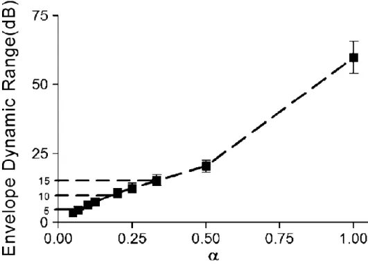
Figure 4.3- The plot of envelope dynamic range (DR) value as a function of compression factor α, which takes the values from 0.05 to 1 corresponding to different DR values. ... 57 Figure 4.4- The histograms for the DR values of the eight temporal envelopes in the 240 vocoded

(9)

viii

factor a, which takes the values of 1/13 (DR = 5 dB; Panel A), 1/5 (DR = 10 dB; Panel B), 1/3 (DR = 15 dB; Panel C), and 1 (Panel D). The dotted line in each subplot fits the histogram of the envelope DR values

using a normal distribution function with parameter values of mean (μ) and standard deviation (σ)... 60

Figure 4.5- Mean recognition scores for (A) Mandarin sentence and (B) Mandarin tone at signal-to-noise ratio (SNR) levels of 5 and 0 dB by the simulated bilateral and unilateral electric hearing. ... 63

Figure 4.6- The amplitude contours of a recording of the Mandarin Chinese vowel /a / in four tones when the DR of the envelope is the original value (Panel A) and compressed to 15 dB (Panel B) and 10 dB (Panel C). ... 65

Figure 4.7: Tone identification scores and standard errors averaged over the three vowels as a function of listening conditions (Quiet, and SNRs of 5 and 0 dB) for the female (top) and male (bottom) speaker. ... 77

Figure 4.8: Tone identification scores and standard errors as a function of the four tone categories in quiet for the female (left panels) and male (right panels) speakers with the three vowels /i/ (top panels), /ɣ/ (middle panels), and /ɑ/ (bottom panels), for six harmonic conditions (All: all harmonics included; High: high harmonics; Low: low harmonics; H1: the first harmonic; H2: the second harmonic; H3: the third harmonic). ... 79

Figure 4.9: Tone identification scores and standard errors as a function of the four tone categories in the noisy listening condition of SNR at 5 dB. The layouts and symbols are the same with Figure 4.8. ... 80

Figure 4.10: Tone identification scores and standard errors as a function of the four tone categories in the noisy listening condition of SNR at 0 dB. The layouts and symbols are the same with Figure 4.8 ... 82

Figure 4.11: The LPC long-term spectrum for the 10-s six-talker Mandarin babble using a sampling frequency of 12207 Hz with the RMS level at 70 dB SPL ... 88

Figure 4.12: The sigmoidal fitting function of tone identification as a function of local SNRs for clustered H1 and H2 (top; R=0.86, p<0.05) and for H3 (bottom; R=0.65, p<0.05). ... 88

Figure 4.13- The sigmoidal fitting function of tone identification as a function of SNRs for the low (R=0.77, p<0.05) and high (R=0.52, p<0.05) harmonics. ... 89

Figure 5.1 Top side shows position of preprocessing technique in signal processing of cochlear implants; Bottom side shows noise reduction on noisy Electrical envelopes. ... 96

Figure 5.2 Block diagram of single-microphone noise reduction methods based on preprocessing the noisy acoustic input signals. ... 97

Figure 5.3 describes the envelope-weighting strategy block diagram. ... 101

Figure 5.4 Block diagram of single-microphone noise reduction methods based on attenuating the noisy electrical envelopes through envelope-selection ... 105

Figure 5.5 the block diagram of traditional MFCC features extraction. ... 108

Figure 5.6 shows the frame with 400 samples length and frame step 160 samples ... 109

Figure 5.7 shows 10 Mel filter-banks start from 300Hz and ends at 8000Hz ... 112

Figure 5.8: Comparison of the traditional MFCC (left) with the integrated approach (right) [82]. ... 115

Figure 5.9 shows Training and transformation stage for Multi-GMM Voice conversion. ... 116

Figure 5.10 block diagram of submodules in Multi-Channel process ... 117

Figure 5.11 Phoneme Segmentation with Praat ... 118

Figure 5.12 Epoch detection in Praat ... 120

(10)

ix

Figure 5.14: multi-channel VC with artificial neural network ... 124 Figure 5.15: Best validation performance is 0.05669 at epoch 4, Blue line shows the decreasing error on training data, Green shows error on Validation data and red shows the error on test data. ... 125 Figure 6.1: compares the quality of Single band and multiband with GMM and ANN methods. ... 126 Figure 6.2: compares the quality of a various number of channels. ... 127

(11)

x

LIST OF TABLES

Table 1.1: lower and upper frequencies in the 16 bandpass filters ... 7 Table 4.1- Filter cutoff (–3 dB) frequencies used for the channel allocation. ... 59 Table 4.2: Fundamental frequency (F0), F1, and F2 frequency (Hz) of the three vowels with four tones. 74 Table 4.3: Results of four-factor (F0 value × vowel category × tone category × stimulus harmonic)

repeated-measures ANOVAs and Tukey post hoc tests in quiet, and the SNR of 5 and 0 dB. DF: degree of freedom; F: Female; M: Male; Hi: High; Lo: Low. ... 84 Table 4.4: Results of three-factor (F0 value × vowel category× stimulus harmonic) repeated-measures ANOVAs for each of the four tones in the SNR of 5 dB. DF: degree of freedom; F: female; M: male; Hi: high; Lo: low. ... 85 Table 4.5: Results of three-factor (F0 value × vowel category × stimulus harmonic) repeated-measures ANOVAs for each of the four tones in the SNR of 0 dB. DF: degree of freedom; F: female; M: male; Hi: high; Lo: low. ... 86 Table 4.6: Confusion matrix of tone identification in quiet for the six harmonic conditions and two talkers (female: left; male: right). ... 87 Table 4.7: Confusion matrix of tone identification at the SNR of 5 dB for the six harmonic conditions and two talkers (female: left; male: right). ... 87 Table 4.8- Confusion matrix of tone identification at the SNR of 0 dB for the six harmonic conditions and two talkers (female: left; male: right). ... 88 Table 4.9: Average amplitude (dB SPL) over the four tones for individual low-frequency harmonics (H1, H2, and H3) for the three vowels and for the female and male speaker. ... 92 Table 5.1 shows frequency and corresponding Mel values for 10 filter-banks. ... 111 Table 5.2 result of phoneme segmentation section ... 119

(12)

1

Chapter One – INTRODUCTION

What is Speech?

Speech is the vocalized form of communicating. Speech signal, produced by muscle actions in the head, neck and using the lungs and the vocal folds in the larynx. In this process air is forced from the lungs through the vocal cords and vocal tract then produced at speaker’s mouth. Speech consists of the following:

Articulation: is the movement of the tongue, lips and other speech organs in order to make speech sound.

Voice: The use of the vocal folds and breathing to produce sound.

Fluency: The rhythm, intonation, stress, and related attributes of speech.

(13)

2

Normal Hearing

The hearing process starts with catching waves by outer area of the ear. Outer ear helps us to determine the direction of a sound. Next sound travels through 10 mm wide ear canal and reaches to the eardrum and causes it to vibrate. Drum vibrates and shakes three small bones in the middle ear that cause amplify signal 22 times and transfer it to Cochlear (figure 1.2).

(14)

3

Cochlear Implants and its structure

People have severe to profound hearing loss in a different age; this may happen by diseases, accident, age or Innate. Hearing loss can be categorized by which part of the auditory system is damaged. There are three basic types of hearing loss: conductive hearing loss, sensorineural hearing loss, and mixed hearing loss. For many years, researchers could not find a solution to restore hearing to profoundly deafened individuals. But starting from the seventies, scientists have been able to make progress in restoring hearing sensation to profoundly deafened individuals by electrically stimulating the auditory neurons.

Fortunately these days, cochlear implant, can be surgically implanted into the inner ear and provide a hearing sensation to a person who is profoundly deaf or severely hard of hearing. It's often referred to as a bionic ear. Cochlear implants can restore hearing in patients suffering deafness due to loss of sensory hair cells in their cochlea. Figure 1.3 shows the cochlear implants. Some people have cochlear implants in both ears

(bilateral), and some just have in one ear (unilateral). Cochlear implants often represent speech formants quite well and enable patients to have telephone conversations unaided.

(15)

4

Not all patients with hearing problems are candidates for cochlear implantation. They need to meet certain audiological criteria. First, the hearing deficiency has to be very severe in one or both ears and receive little or no benefit from hearing aids. Profound deafness [1], generally defined as a hearing loss of more than 90 dB, and hearing loss is typically measured as the average of pure tone hearing thresholds at octave frequencies. Second, the candidate has to score 65% or less on sentence recognition tests done by hearing professional in the ear to be implanted. Since 2000, cochlear implants have been FDA-approved for use in eligible children beginning at 12 months of age.

Over decades, several cochlear implant devices have been developed, and all of them have the following components:

1. The microphone that converts sounds into electrical signals.

2. The sound processor that modifies acoustic signals for the purpose of auditory stimulation.

3. The radio-frequency link that transmits the electrical signals to the implanted electrodes. 4. An electrode or an electrode array (consisting of multiple electrodes) that is inserted into the

cochlear by a surgeon during a surgery.

Figure 1.4 describes different section of cochlear implant device.

(16)

5

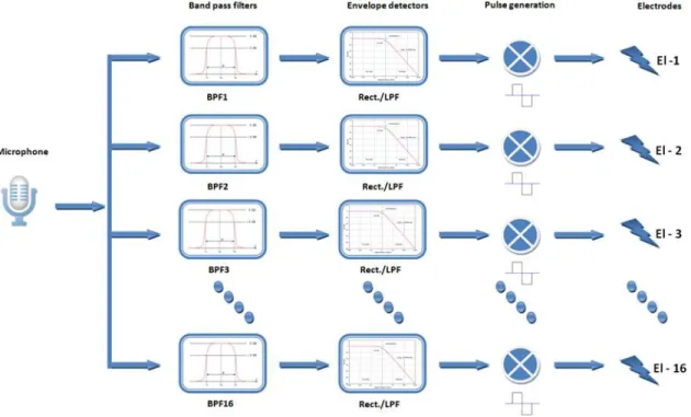
In single-channel implants, only one electrode is used. However, in multi-channel cochlear implants, an electrode array that typically consists of 16-22 electrodes is inserted into the cochlea. Thus more auditory nerve fibers can be stimulated at different places in the cochlea(e.g., Shannon et al. [2], Dorman et al. [3]). Different electrodes are stimulated depending on the frequency range of the acoustic signal. Electrodes near the base of the cochlea are stimulated with high-frequency signals while electrodes near the apex are stimulated with low-frequency signals. The primary function of the signal processor is filtering the input signal into different frequency bands or channels and delivering the filtered signals to the assigned electrodes. The sound processor is used to analyze the acoustic signal into different frequency components, similar to the way healthy cochlear processes acoustic signals.

(17)

6

Multi-channel cochlear implants consist of multiple bandpass filters. The total number of bandpass filters is denoted, as the total number of channels. For example, if we have 16 channels we need to have 16 bandpass filters. The Frequency bandwidth for each channel is different from the others and defined in logarithmic scale. The range of frequency is arbitrarily set between 350Hz to 5500Hz for the simulation purposes. Figure 1.6 shows 16 band pass filter.

Band boundaries can be calculated as below:

Range=log (𝑈𝑝𝑝𝑒𝑟_𝐹𝑟𝑒𝑞𝑢𝑒𝑛𝑐𝑦 𝐿𝑜𝑤𝑒𝑟_𝐹𝑟𝑒𝑞𝑢𝑒𝑛𝑐𝑦) (1-1) Interval= 𝑅𝑎𝑛𝑔𝑒 𝑁𝑢𝑚𝑏𝑒𝑟_𝑜𝑓_𝐶ℎ𝑎𝑛𝑛𝑒𝑙𝑠 (1-2) Upper_Bandi = 𝐿𝑜𝑤𝑒𝑟_𝐹𝑟𝑒𝑞𝑢𝑒𝑛𝑐𝑦 ∗ 10𝐼𝑛𝑡𝑒𝑟𝑣𝑎𝑙∗𝑖 (1-3) Lower_Bandi = 𝐿𝑜𝑤𝑒𝑟_𝐹𝑟𝑒𝑞𝑢𝑒𝑛𝑐𝑦 ∗ 10𝐼𝑛𝑡𝑒𝑟𝑣𝑎𝑙∗(𝑖−1) (1-4)

(18)

7

16 channels bandpass filters shows in table 1.1

Lower Band Center Upper Band

Channel 1 350 Hz 382.87 Hz 415.75 Hz Channel 2 415.75 Hz 454.80 Hz 493.86 Hz Channel 3 493.86 Hz 540.25 Hz 586.64 Hz Channel 4 586.64 Hz 641.74 Hz 696.85 Hz Channel 5 696.85 Hz 762.31 Hz 827.77 Hz Channel 6 827.77 Hz 905.52 Hz 983.28 Hz Channel 7 983.28 Hz 1075.64 Hz 1168.01 Hz Channel 8 1168.01 Hz 1277.72 Hz 1387.44 Hz Channel 9 1387.44 Hz 1517.77 Hz 1648.10 Hz Channel 10 1648.10 Hz 1802.91 Hz 1957.72 Hz Channel 11 1957.72 Hz 2141.62 Hz 2325.52 Hz Channel 12 2325.52 Hz 2543.96 Hz 2762.41 Hz Channel 13 2762.41 Hz 3021.90 Hz 3281.38 Hz Channel 14 3281.38 Hz 3589.62 Hz 3897.85 Hz Channel 15 3897.85 Hz 4263.99 Hz 4630.14 Hz Channel 16 4630.14 Hz 5065.07 Hz 5500 Hz

(19)

8

In cochlear implants, only temporal envelope information is delivered to the auditory neurons. We use envelope detection to generate the output signal for each channel. A common and efficient technique for envelope detection is based on the Hilbert Transform.

In our implementation after bandpass filtering, we use the low pass filter to detect envelop. Our cutoff frequency in discrete-time domain is calculated as below:

Lpf =400 Hz, (1-5)

Fs= sampling frequency (1-6)

W0= Lpf/Fs (1-7)

After calculating filter parameters, we use them to generate filtered signal from absolute values of bandpass filtered signals. Ultimately, we modulate the envelope signals to biphasic pulse carriers and deliver them to electrodes. Figures 1.7, 1.8, 1.9 and 1.10, shows different channels for signal “ASA” and envelope detection for each of them.

(20)

9

Figure 1.8: Channels 5 to 8 signals and envelop

(21)

10

Figure 1.10: Channels 13 to 16 signals and envelop

As can be seen, envelope signal is quite different from the original signal. The problem at hand is how to use normal hearing subjects to test the stimuli heard by the CI user? For simulation purposes, we modulate “white noise” carrier to the envelope signals.

(22)

11

Patient difficulties and limitations

Cochlear Implants can restore sufficient hearing for patients who has profound hearing loss in both ears and allow them to understand of speech in a quiet background. However, they still have serious problems in understanding speech in noisy environments, such as restaurant, airport, and classroom. Several studies show in the presence of background noise, the speech recognition of CI listeners is more sensitive to background noise than that of normal-hearing (NH) listeners. This phenomenon is most likely because of the limited frequency, temporal, and amplitude resolution that can be transmitted by the implant device (Qin & Oxenham, 2003[4]). In fact, a combination of weak frequency and temporal resolution and channel interaction (or current spread) in the stimulating electrodes are some of the reasons implant users have difficulty in recognizing speech in noisy environments. These factors raise the difficulty of hearing in noisy conditions for CI users, regardless of the type of noise (e.g., steady-state or modulated) present (e.g., see Fu & Nogaki, 2004[5]). In the study by Firszt et al. (2004)[6], speech recognition was assessed using the Hearing in Noise Test (HINT) sentences (Nilsson, Soli, & Sullivan, 1994 [7]). Results revealed that CI recipients’ performance on sentence recognition tasks in a present of noise was significantly lower than listening at a soft conversational level in quiet.

Present implants are unable to deliver complete temporal and spectral fine structure information to allow implanters to enjoy pitch and musical melody, or to localize sound sources accurately. These limitations make it hard for patients to follow conversations in environments with high background noise.

(23)

12

Chapter Two - Objectives and Motivation

There is no doubt that human life depends on relation and communication with other peoples. Interaction is fundamental to mankind society. “People’s participation is becoming the central issue of our time,” says UNDP in its Human Development Report 1993. Thousands of research and reports show benefits of communication in our daily life. Communication is the root of human sociality since beginning till now, and visiting a relative or friend is essential in social activities. Talking and listening is a core of communication and most people believe that talking to friends and family is very delightful. Some peoples consider the comfortable conversation with family is the primary factor and make it pleasant. However, better perception and understanding can be another reason to attract people to communicate with a familiar person.

An earlier study has revealed that familiarity with a talker’s voice can improve understanding of the conversation. Research has shown that when adults are familiar with someone’s voice, they can more accurately – and even more quickly – process and understand what the person is saying. This theory, identified as the “familiar talker advantage,” becomes into action in locations where it is difficult to hear. For example, in a loud or crowded place, adults can better understand those whose voices they already know [8].

In some cases, manipulation of the talker dimension been shown to improve linguistic performance. Individual research by Magnuson(1995) [9], Nygaard and Pisoni(1998) [10] and Sommers(1994) [11] shows, familiar talkers, improved word recognition in adult speech perception. In those researches, they trained listeners with a set of speakers once subjects are

(24)

13

familiar with talkers’ voices; they perform a linguistic processing task such as word recognition or sentence transcription. These studies have shown that normal hearing listeners’ performance on the linguistic tasks with familiar talkers is consistently better than unfamiliar talkers. Figure 2.1 shows the result of research conducted by Nygaard L. C., Sommers M. S., and Pisoni D. B. (1994) [11]. Mean intelligibility of words presented in noise for trained and control subjects in four SNR levels (-5dB, 0dB, +5dB and +10dB). Trained, or experimental, subjects were trained with one set of talkers and tested with words produced by these familiar talkers. Control subjects were trained with one set of talkers and tested with words produced by a novel set of talkers.

(25)

14

In research was done by Levi, Winters and Pisoni [8]; Native talkers in two languages (English and German) who were unfamiliar to all listeners selected. Also, listeners divided into four groups based on language and their ability to voice learning. Then listeners trained in six sessions for three days. They assessed the performance of each session by percentage of speaker identification. These results are shown in Figure 2.2.

Figure 2.2:Talker identification accuracy during the six training sessions for both German-trained and English-trained listeners separated by good and poor voice learners. Two training sessions were completed on each day of training. by Levi, Winters and Pisoni [8].

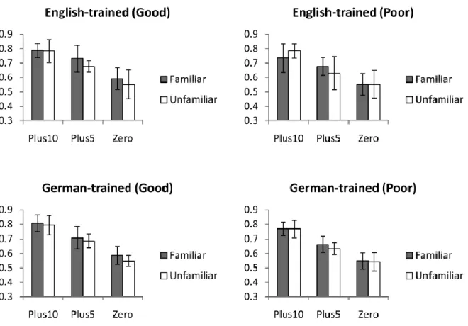
Response obtains based on proportion of correct phonemes in three SNR levels (0dB, +5dB and +10dB) to familiar and unfamiliar talker in both languages. Figure 2.3 shows their results.

(26)

15

Figure 2.3:Proportion phonemes correct by SNR for English-trained and German-trained learners divided by learning ability (good and poor). Levi, Winters and Pisoni [8].

In a study issued by Hazan and Markham (2004)[12], conducted single word materials

(124 words) from 45 talkers (from a homogeneous accent group) and presented to 135 adult and child listeners in low-level background noise. It appears that word intelligibility was considerably related to the total energy in the 1- to 3-kHz region and word duration. Also shows that the relativistic intelligibility of different talkers was very consistent across listener age groups. That implies the acoustic-phonetic characteristics of a talker's speech are the primary factor in determining talker understandability.

Several reports have shown that listeners are highly sensitive to the talker dimension, and it’s been proven that knowledge about a talker alters segmental perception. (Ladefoged and

(27)

16

Broadbent, 1957[13]; Ladefoged, 1978[14]; Johnson, 1990[15]; Johnson et al. 1999[16]; Allen and Miller, 2004[17]; Eisner and McQueen, 2005[18]; Kraljic and Samuel, 2005, 2006, 2007[19][20][21]; Kraljic et al., 2008[22]). Also similar studies for cochlear implant users show CI users are sensitive to different talkers. For example Green et al. (2007) [23] investigated the effects of cross-talker on speech intelligibility in CI users, and normal hearing listeners were listening to acoustic CI simulations. They select two groups of talkers each group consisted of one male adult, one female adult, and one female child. These groups were divided consider to previous data collected with NH listeners according to mean word error rates (high or low intelligibility talkers). Results explained differences in understandability between the two talker groups, for different conditions

The aim of this research is to develop algorithms which can convert speech from one speaker to another one. Based on previews studies Voice conversion algorithms can use to generate familiar talker for cochlear implant (CI) users. This voice can be a voice of family member or friends who have the highest performance of intelligibility for CI user.

(28)

17

Chapter Three - Introduction to Voice Conversion and algorithm

Voice Conversion, which is also mentioned as voice transformation and voice morphing, is a technique to alter a source speaker's speech statement to sound as target speaker. In other words, it refers to a system of changing a person's voice to either make them sound like someone else or to pretend their voice. In voice conversion technique we may change the tone or pitch, add distortion to the user's voice, or a combination of all of the above to reshape the structure of sound and have similar characteristics to another speaker.

Figure 3.1:Concept of Voice conversion.

There are many applications which may benefit from this sort of technology. For example, a Text To Speech system with voice morphing technology combined can generate various voices. In TTS systems, synthesized speech can be formed by concatenating pieces of recorded speech that are filed in a database. With Voice Conversion technique we can extend these databases and create numerous voices. Another case can be anywhere that the speaker character can change, such as dubbing movies and TV-shows, computer games and cartoons the

(29)

18

availability of high-quality voice morphing technology will be very worthy because allowing the fitting voice to be generated without the real actors being present.The other application of using this technique is voice restoration system. People who have lost or damage their speech system can use this device to communicate.

All of the applications mentioned above are assume that both source and target speakers, talk in the same language. However, cross-language voice conversion system assumes that source and target speakers use different languages. In this method timbre or the vocal identity of speaker replace in recorded sentences. [24]

Based on those applications we can divide voice conversion technique to two categories:

- Text-dependent or parallel recording

- Text-independent or non-parallel recording

In Text-dependent systems, the set of utterances recorded by both source and target speakers use as training material to create conversion model. On the other hand, in the text-independent application such as the cross-lingual voice conversion, speakers talk in different languages so it focuses on timbre and acoustic feature of speech.

The process of voice conversion contained two stages:

 Training stage

 Transforming stage

In the training phase(First stage), a set of parallel materials usually refers to a list of sentences covered all phonetic content of language enter as input then aligned for synchronous feature extraction and conversion model creation. Acoustic feature extraction usually down

(30)

19

frame-by-frame and 15ms or 25ms commonly select for each frame length. In order to have high-quality data, the sample rate of 8 kHz and 16 kHz with 16 bits or more sample required. Figure 3.2 shows two stages of voice conversion system.

Figure 3.2 shows two stages of voice conversion system.

In the second stage or transformation step, source speech converts to target speech by the model created in the training stage.

(31)

20

Voice Conversion Techniques

For the first time Childers et al.[25] introduced Voice conversion (VC) in 1985. In his paper, he proposed a method that includes mapping acoustical features of the source speaker to the target speaker. In 1986, Shikano[26] offered to use vector quantization(VQ) techniques, and codebook sentences. In 1992, Valbert[27] proposed personalized Text to Speech using Dynamic Frequency Warping(DFW). Seven years later Stylianou[28] introduced Gaussian Mixture Models(GMMs) merged with Mel-Frequency Cepstral Coefficients(MFCCs) for Speaker transformation algorithm. Also, Rentzosin in 2003[29], Ye in 2006[30], Rao in 2006[31] and Zhang in 2009[32] have concentrated on probabilistic techniques, such as GMMs, ANN and codebook sentences.

The transformation stage in voice conversion systems is concerned all acoustic feature applied in the voice signal. Such as pitch shifting and energy compensation. A. F. Machado and M. Queiroz. In Voice conversion: A critical survey [33] categories all transformation techniques in four groups:

 Linear Algebra Techniques

 Signal Processing Techniques

 Cognitive Techniques

(32)

21

Linear algebra techniques

Linear algebra techniques such as Bilinear Models, Linear predictive coding (LPC), Singular Value Decomposition (SVD), Weighted Linear Interpolations (WLI) and Perceptually Weighted Linear Transformations, and Linear Regression (LRE, LMR, MLLR) are based on geometrical interpretations of data. For example in finding simplified models by orthogonal projection (linear regression), in getting linear combinations of input data (weighted interpolations), or in decomposing transformations into orthogonal components (SVD).

Linear predictive coding (LPC) is a mechanism frequently adopted in audio signal processing, and speech processing such as speech synthesis, speech recognition, and voice conversion. This method used the information of a linear predictive model in the compressed form of a digital signal of speech for representing the spectral envelope. It is one of the most useful methods for encoding good quality speech at a low bit rate and provides extremely accurate estimates of speech parameters and one of the simplest methods of predicting projected values of a data set.It is using previous data in series to predict the next value in a sequence. In this technique, we assume we can learn the behavior of the sequence from a chunk of training information, and then we can apply our learning to places where the next point is unknown. The number of previous points we use to predict the next item in a sequence known as the order of LPC model. For example, if 4 data points are used to predict a fifth one, then we call it an order 4

model. Thetypical vocal track model an all-pole LTI system.

𝐻(𝑧) = 1

1 + 𝑎1𝑧−1+ 𝑎2𝑧−2+ 𝑎3𝑧−3+ ⋯ + 𝑎𝑝𝑧−𝑝

(33)

22

𝐻(𝑧) = 1

1 + ∑𝑝_𝑘=1𝑎𝑘𝑧−𝑘

Where p is the prediction order and the typical value of p are from 8 to 12 (two linear prediction coefficients for each dominant frequencies "formants"). For the signal y(n) an autoregressive(AR) model shown below:

y(n) = e(n) - a1y(n-1) - a2y(n-2) - a3y(n-3) - … - apy(n-p)

Which e(n) is excitation signal.

e(n) H(z) y(n)

The goal is for each given speech signal s(n), find the excitation signal e(n) and coefficients ak to

generate y(n) close to signal s(n). Thus, we can store coefficients ak and excitation signal e(n) to

represent signal s(n). Steps to create LPC model shown in figure below:

(34)

23

In order to calculate LPC coefficients for each frame f(n), first we need to calculate the autocorrelation of f(n):

corr(n) = f(n)*f(n-1)

Then solve the Yule-Walker equation [34]. Example below shows Yule-Walker equation for p=4

[ 𝑐𝑜𝑟𝑟(0) 𝑐𝑜𝑟𝑟(1) 𝑐𝑜𝑟𝑟(2) 𝑐𝑜𝑟𝑟(3) 𝑐𝑜𝑟𝑟(1) 𝑐𝑜𝑟𝑟(0) 𝑐𝑜𝑟𝑟(1) 𝑐𝑜𝑟𝑟(2) 𝑐𝑜𝑟𝑟(2) 𝑐𝑜𝑟𝑟(1) 𝑐𝑜𝑟𝑟(0) 𝑐𝑜𝑟𝑟(1) 𝑐𝑜𝑟𝑟(3) 𝑐𝑜𝑟𝑟(2) 𝑐𝑜𝑟𝑟(1) 𝑐𝑜𝑟𝑟(0)] [ 𝑎₁ 𝑎₂ 𝑎3 𝑎4 ] = − [ 𝑐𝑜𝑟𝑟(1) 𝑐𝑜𝑟𝑟(2) 𝑐𝑜𝑟𝑟(3) 𝑐𝑜𝑟𝑟(4) ]

Next step after generating H(z) for each frame is computing the excitation signal.

y(n) 1/H(z) e(n)

1/H(z) is an FIR filter thus excitation signal calculate by filtering s(n) with FIR filter 1/H(z).

We can perform voice conversion by replacing the excitation component from the given speaker with a new one. Since we are still using the same transfer function H(z), the resulting speech sample will have the same voice quality as the original. However, since we are using a different excitation component, the resulting speech sample will have the same sounds as the new speaker.

Signal processing techniques

Signal processing techniques refer to methods such as Vector Quantization (VQ) and Codebook Sentences, Speaker Transformation Algorithm using Segmental Codebooks (STASC), and Frequency Warping (FW, DFW and WFW) which represent transformations based on time-domain or frequency-time-domain representations of the signal. This group of methods encodes a

(35)

24

signal using libraries of signal segments or code words. The other member of this family transforms timbre-related voice features by altering frequency scale representations.

Before we review voice conversion in this group, we need to describe some of the algorithms has an important impact on all techniques. Dynamic time warping (DTW) is an algorithm for measuring the relationship between two temporal series which may vary in time or speed. For example, Finding walking pattern between to person even one of them walks faster than another one. In fact, any type of data such as Audio and Video can be transformed into a linear sequence then analyzed by DTW. In definition, DTW is an algorithm that estimates an optimal similarity between two given sequences (e.g. time sequences) with specific limitations. To measure a correlation between sequences in the time domain, the sequences are "warped" non-linearly. Dynamic frequency warping (DFW) is an exact analog of dynamic time warping (DTW) which is used to reduce the difference in frequency scale of speech and normalize the frequency correctly.

(36)

25

Vector quantization (VQ) is one of the classic signal processing techniques that used for data compression. This method uses the distribution of prototype vectors for modeling of probability density functions. In this technique, large vectors (set of points) separated into groups owning almost the same number of points nearest to them. Each group is expressed by its centroid point same as k-means and some other classification algorithms. In 1986, Shikano[26] introduced the speaker adaptation algorithms which use VQ codebooks of two representatives(input speaker and reference speaker). In this method, vectors in the codebook of

a reference speaker exchange with vectors of the input speaker's codebook.Abe et al.(1988)[36]

present voice conversion method based on a speaker adaptation method by Shikano et al. (1986). This method relies on producing a discrete mapping between source and target spectral envelopes. This algorithm contains two stages: learning stage and converting stage.

(37)

26

Figure 3.5 shows each step of this method. This method requires parallel recordings from both speakers (source and target) as input to learning stage. The first step is generating spectral vectors for all recordings (in this case Mel-frequency cepstral coefficients).The second step, creating vector quantization (VQ) of each speaker. In next step frames of each sentence align respect to another speaker by using dynamic time warping (DTW) then similarity vector between two speakers store as a 2D histogram. And in the last step of learning stage, it generates mapping codebook for both pitch and energy of speaker B (a linear combination of speaker’s B vectors) by using each histogram as a weighting function.

In Transform stage, First step is, Create VQ of input speech with respect to spectrum and pitch. Next use mapping codebook to decode (convert) parameters of speaker A to the speaker B. and at last synthesis (reconstruct) the new speech.

Another famous technique in this group is Pitch Synchronous Overlap and Add (or PSOLA). PSOLA is digital signal processing method used for speech synthesis, and it can be used to modify the pitch and duration of a speech signal. In PSOLA algorithm speech waveform divided into the small overlapping sections. To increasing the pitch of signal, the segments must move closer to each other and to decreasing the pitch of signal distance between segments has to increment. In the same way, to increase the duration of the signal, the segments has to copy multiple times and to decrease the duration, some of the segments have to eliminate. After that, remaining segments merged again using the overlap-add technique.

(38)

27

Figure 3.6 shows increasing (a) and decreasing (b) of pitch with PSOLA method.

In 1992 Valbert et al.[27] introduced voice conversion method using all above methods together. Key steps in this approach listed below:

 Divided parallel recording of both speakers (source and target) to frames.

 Align frames using DTW and correlate pairs.

 Extracting pitch marks for each set of speech.

 Vector quantize of source frames

 Build a dynamic frequency warp (DFW) for each cluster between source and

(39)

28

 adjusting pitch and duration using LP-PSOLA

Cognitive techniques

Cognitive techniques cover all methods that using abstract neuronal structures, and usually depend on a training phase such as Artificial Neural Networks (ANN), Radial Basis Function Neural Networks (RBFNN), Classification and Regression Trees (CART), Topological Feature Mapping, and Generative Topographic Mapping. It is necessary to both inputs, and outputs are available. Usually, they are used for cases that only two possible output values are available. One of the good examples of these decision problems is speech recognition. For solving this problem we need separate network (model), trained for each specific phoneme or word or sentence that is going to be recognized.

(40)

29

Artificial Neural Network (ANN) algorithms are machine learning and cognitive science technique which are used to compute functions that can depend on a lot of inputs and are regularly unknown. These models include interconnected "neurons" which exchange data between each other. The connection between two nodes has a weight associated with it that can be tuned based on learning. In 2009 Srinivas et al. [35] offer to use this technique(ANN) for Voice conversion. The ANN is trained to convert Mel-cepstral coefficients (MCEPs) of the source speaker to the target speaker's MCEP's. That approach used a parallel set of sentences from source and target speakers. In feature extraction step, MCEPs and fundamental frequency extract as filter parameters and excitation feature. In next step, dynamic time warping is used to align MCEP vectors between the source and target speakers. The output of this stage is set of paired feature vector X and Y which used to train ANN model to perform the transforming from X to Y.

(41)

30

Statistical Techniques

Statistical Techniques include Gaussian Mixture Models (GMM), Hidden Markov Models (HMM), Multi Space Probability Distributions, Maximum Likelihood Estimators (MLE), Principal Component Analysis (PCA), Unit Selection (US), Frame Selection (FS), K-means and K-histograms. In this group, some of the techniques such as Gaussian model assume feature vectors or vocal parameters have a random component and may be expressed by means and standard deviations. The other group such as Markov models develops over time according to simple rules based on the recent past.

Figure 3.9 a) Shows GMM classification. b) Shows HMM model

A Gaussian Mixture Model (GMM) is a parametric probability density function represented as multiple Gaussian distributions (Distribution based on population mean and the variance). GMM is one of the famous signal processing techniques that use for speaker recognition and in voice conversion system known as the state of the art technology because it

(42)

31

has the best quality of transformed speech. GMM parameters are estimated from well-trained datasets using the iterative Expectation-Maximization (EM) algorithm.

The probability density of the Gaussian distribution shown in equation below:

f(x|μ, σ2) = 1 σ√2πe −(x−μ)2 2σ2 Where - x is data point.

- μ is mean or expectation of the distribution:

μ = 1 M∑ Xi

M

i

- 𝜎 is Standard Deviation and 𝜎2_{is Variance}

σ2 = 1

M∑(Xi− μ)

2 M

i

(43)

32

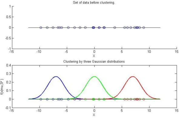
To demonstrate GMM we can use a set of data shown in figure 3.11 (a). That data doesn't like one Gaussian, and it looks like we have three groups of data. Figure 3.11(b) shows simple Gaussian Mixture Model that involves three Gaussian distributions.

Figure 3.11 Gaussian Mixture Model

GMM has a probability distribution that indicates the probability that each point belongs to the cluster. There are various techniques available for determining the parameters of a GMM. A General Gaussian mixture model is the linear combination of several Gaussian functions given by the equation below:

𝑝(𝑥_𝑖|𝛾) = ∑ 𝜔𝑖𝑓(𝑥|𝜇𝑖, 𝜎𝑖2) 𝑘

(44)

33

Where x is continuous-valued data vector (features), k is the number Gaussian distribution, ω_i (i = 1 . . K) are prior probabilities or the mixture weights, 𝛾 is set of mixture model with k components ({μ₁, σ₁2_{, 𝜔}

1}, {…}, {μK, σK2, 𝜔𝐾}) and f(x|μi, σi2) are Gaussian densities given in equation below:

𝑓(𝑥|𝜇_𝑖, 𝜎_𝑖2_{) =} 1

𝜎_𝑖√2πe

−(x−𝜇𝑖)

2

2𝜎𝑖2

One of the most popular methods for Parameter Estimation and unsupervised learning is Expectation-Maximization (EM). Expectation-Maximization (EM) is a parameter estimation algorithm for GMMs that will determine an optimal setting for all of the GMM parameters, using a set of data points. EM algorithm start with initializing each Gaussian model randomly (𝜇, 𝜎 𝑎𝑛𝑑 ω), then estimate a new model base on initial one. After that, the new model becomes the initial model for the next iteration, and it will continue until convergence. Figure 3.12 shows parameter estimation for GMM using EM algorithm.

(45)

34

In Expectation stage, for each input data 𝑥𝑖 and Gaussian mixture kth(m1…mK),

probability density needs to compute. The formula below used to derive posterior probability or membership weight:

𝑝(𝑥𝑖|𝛾𝑘) =

𝜔_𝑘𝑓(𝑥|𝜇_𝑘, 𝜎_𝑘2₎

∑𝐾 𝜔_𝑚𝑓(𝑥|𝜇_𝑚, 𝜎_𝑚2₎ 𝑚=1

Where 𝑥_𝑖 is from training vector x={x1… xM} and 𝜔𝑘 is weights for mixture kth. In Maximization stage, a new value (𝜔_𝑘 , 𝜇_𝑘 and𝜎_𝑘) for each mixture needs to re-estimate (update). The equations in the Maximization stage required to be calculated in this order, first compute the M new Mixture weight, then the M new means, and finally the M new Variances. Equations below show estimation formula for 𝜔_𝑘 , 𝜇_𝑘 , and 𝜎_𝑘.

Prior probabilities or Mixture weight:

𝜔_𝑘 = 1

𝑀∑ 𝑝(𝑥𝑖|𝛾𝑘)

𝑀

𝑖=1

Mean (calculate 𝜇_𝑘𝑛𝑒𝑤 for all mixtures):

𝜇_𝑘𝑛𝑒𝑤 =∑ 𝑝(𝑥𝑖|𝛾𝑘) ∗ 𝑥𝑖

𝑀 𝑖=1

∑𝑀 𝑝(𝑥_𝑖|𝛾_𝑘)

𝑖=1

Variance (used new 𝜇 calculated in last step):

𝜎𝑘 =

∑𝑀 𝑝(𝑥_𝑖|𝛾_𝑘) ∗ (𝑥_𝑖 − 𝜇_𝑖𝑛𝑒𝑤)2 𝑖=1

(46)

35

Convergence is commonly recognized by measuring the value of the log-likelihood at the end of each iteration and declares finish when there is no significant change between current and last iteration. We can compute the log-likelihood as defined below:

𝑙(𝛾) = ∑ 𝑙𝑜𝑔 ( ∑ 𝑝(𝑥_𝑖│𝛾_𝑚) 𝐾 𝑚=1 ) 𝑀 𝑖=1 = ∑ (𝑙𝑜𝑔 ∑ 𝜔_𝑚𝑓(𝑥_𝑖|𝜇𝑚, 𝜎𝑚2) 𝐾 𝑚=1 ) 𝑀 𝑖=1

Where M is a number of data points, K is a number of mixtures (Gaussian component), and p is the Gaussian density for the mth mixture component.

In 1998 Stylianou et al. [28] proposed the Gaussian Mixture Model (GMM) for Voice Conversion. Their approach assumes two sets of parallel speech from both speakers are present. Then from each set, spectral envelope (e.g., MFCC) extracted with a fixed 10ms frame rate and aligned using Dynamic Time Warping (DTW). In next step GMM model generate for source data by using Expectation-Maximization (EM) algorithm. And in the final step of learning procedure conversion function generate by applying least squares (LS) Optimization. After a transformation function has been computed, the process can be iterated back to re-estimating the time-alignment step between the transformed envelopes and the objective envelopes. Figure 3.13 shows the block diagram of the learning procedure.

(47)

36

In next stage (conversion stage) use PSOLA like modifications to re-computing the pitch-synchronous synthesis. After applying conversion signal to spectral envelopes, results need to filter to eliminate noises. The noise portion is adjusted with two different fixed filters (so-called corrective filters) for voiced and unvoiced frames. Figure 3.14 shows the block diagram of the voice conversion procedure.

(48)

37

Chapter Four – Feature Enhancement

Effects of low harmonics on tone identification in natural and vocoded speech

4-1-1 Introduction

In order to have adequate linguistic communication, for audiences in tone languages same as Mandarin Chinese, the perception of lexical tones is important to understanding word meanings [37]. For example, the syllable [ma] in the Mandarin language can pronounce in four different fundamental frequency (F0) height and contour shapes. And each tone has a different meaning (high-level as tone 1, high-rising as tone 2, low-fall-rise as tone 3, and high-falling as tone 4, means “mother, hemp, horse, and scold,” respectively).[38] F0 height or contour primarily contains the tone information. However, the other cues such as amplitude contour and syllable duration also make contributions. [39][40][41]

When F0 leads are not available such as whispering speech or signal-correlated-noise stimuli, Mandarin-native normal-hearing (NH) audiences were able to recognize Mandarin tones by using temporal envelope cues with an accuracy of 60%–80%[39][40][41]. As a matter of fact, these studies also shows that amplitude contours significantly associated with the F0 contours of natural speech, although such correlations may depend on vowel context, tone category, and speakers. Also, higher correlations between amplitude contours and F0 contours can increase tone identification accuracy.[41] Another study shows that adjusting the amplitude contour to more closely resemble the F0 contour improved tone identification for NH listeners listening to

(49)

38

cochlear implant (CI) simulations. This result shows the influence of amplitude contours on tone identification. [42]

In a later study, Luo and Fu[43] measured Mandarin tone, phoneme, and sentence recognition in steady-state speech-shaped noise for Mandarin Chinese-native speakers listening to an acoustic simulation of binaurally combined electric and acoustic hearing (i.e., low-pass filtered speech in one ear and a six-channel CI simulation in the other ear). Results revealed that frequency information below 500 Hz mostly presented to tone recognition, while frequency information above 500 Hz was important to phoneme recognition.

In this study, we investigate the effect of the low harmonics below or near 500 Hz of Mandarin speech on tone identification for natural and vocoded speech. CI patient’s auditory perception (e.g., temporal modulation detection and pitch perception) depends on a temporal envelope (e.g., amplitude contour) cues because of lack of resolved harmonics and temporal fine structure ([44],[45]). Besides, the cues of F0, harmonic structures, and temporal fine structures above 500 Hz (Refs. [42] and [43]) are not well maintained in CI processing. Therefore, it is important to recognize the contribution of the temporal envelope of the low harmonics (e.g., the first three harmonics, the frequencies of which are below or near 500 Hz) to Mandarin tone recognition with CI processing.

As we know, speech sounds are processed into a number of continuous frequency bands in CIs, a noise-vocoded speech of each of the three low harmonics was used to examine the effects of their amplitude contours on tone recognition. The effect of background noise was also measured, considering that noise may interrupt the temporal properties of speech signals and

(50)

39

low-frequency harmonics. It is assumed that a closer correlation between amplitude contour and F0 contour leads to better tone recognition.

4-1-2-Method 4-1-2-1-Listeners

Ten young Mandarin Chinese-native listeners ranging in age from 20 to 25 years old participated in this study. They had normal hearing sensitivity with pure-tone thresholds less or equal to 15 dB hearing level [46] at octave intervals between 250 and 8000 Hz in both ears. Listeners were paid for their participation. All participants, undergraduate or graduate students in Beijing, China, were from northern China and spoke standard Mandarin. None of the listeners had a formal musical education of more than five years, and no listeners had received any musical training in the past three years.

4-1-2-2-Stimuli

4-1-2-2-1-Speech signal

Four tones of the Chinese vowel /Ç/ were recorded from two young speakers (one female and one male Mandarin native speaker) in isolation forms. The F0 for the female speaker ranged between 160 to 324 Hz and for the male speaker varied between 95 to 215 Hz across the four tones. The average F1 and F2 frequencies of the vowels with four tones were 531 and 1492 Hz for the female speaker and were 430 and 1102 Hz for the male speaker. The duration of each tone was leveled at 210ms, and the vowel signals were normalized to the same root-mean-square (rms) value.

The steps to generate stimuli with individual low-frequency harmonics described as follows. First, vowel signals were segmented into 30ms frames with 50% overlap, and a

(51)

pitch-40

detection algorithm based on an autocorrelation function was used to obtain F0 values in each voiced frame. Second, harmonic analysis and synthesis of the vowel signals were conveyed in the frequency domain using a 2048 point fast Fourier transform. The harmonics identified as magnitude spectrum peaks around the integer multiple of F0. For example, The second harmonic classified as the magnitude spectrum peak around 2*F0. There were four harmonic synthesis conditions: first, three using the three individual harmonics (H1, H2, and H3) and the condition four using all harmonics (i.e., all). Third, the synthesis was implemented by using the overlap-and-add approach for the corresponding harmonic condition. The level of stimuli with all harmonics was set at 70 dB sound pressure level (SPL) for both quiet and noise (i.e., 10 dB signal-to-noise ratio (SNR) for the noise condition). Also, the level of stimuli with individual harmonics classified from 56.7 to 66.7 dB SPL, depending on the rms level of each harmonic relative to the rms level of natural speech with all harmonics.

The stimuli in both quiet and noise conditions vocoded with eight-channel noise-vocoder and described as follows. First, Both clean harmonic signals (i.e., H1, H2, H3, and all) and noisy harmonic signals (i.e., signal and noise were mixed before the vocoded processing) were divided into eight frequency bands between 80 and 6000 Hz using sixth-order Butterworth filters. The cutoff frequencies of the eight channels were set as 80, 221, 426, 724, 1158, 1790, 2710, 4050, and 6000 Hz, respectively. Also, the equivalent rectangular bandwidth scale [47] was used to allocate the eight channels.

In the second step, the temporal envelope was extracted by full-wave rectification and low-pass filtering using a second-order Butterworth filter with a 160 Hz cutoff frequency in each frequency band. White Gaussian noise was modulated by the temporal envelope of each frequency band, followed by band-limiting using the sixth-order Butterworth band-pass filters.

(52)

41

Third, the envelope-modulated noises of each band were added together, and the level of the synthesized vocoded speech was normalized to produce the same rms value as the original harmonic signal.

4-1-2-2-2- Noise

400ms of long term speech shaped (LTSS) noise used as the noise due to its comparison to the spectra of speech signals. Gaussian noise that was shaped by a filter with an average spectrum of Mandarin six-talker babble used to generate the LTSS noise at 60 dB SPL[48]. In noise conditions, the 210ms signal was temporally presented at the center of the 400ms noise.

4-1-2-2-3- Stimulus condition

In this study, five factors considered for generating a total of 128 stimulus conditions:

1. Two talkers (one male and one female)

2. Four harmonic conditions (H1, H2, H3, and all)

3. Two types of speech (natural and vocoded speech)

4. Two listening conditions (quiet and noise with a 10 dB SNR)

5. Four tones (tones 1–4)

4-1-2-3- Stimulus presentation

Digital stimuli, sampled at 12207 Hz, were presented to the listeners’ right ears through MDR-7506 headphones. Listeners were seated in the Psychological Behavioral Test rooms of the National Key Laboratory of Cognitive Science and Learning at Beijing Normal University. A

(53)

42

Tucker-Davis Technologies (TDT) mobile processor (RM1) was used for the stimulus presentation. The SPLs of acoustic stimuli were calibrated in a NBS 6 cm3 coupler using a Larson-Davis (Depew, NY) sound-level meter (Model 2800) to set the linear weighting band.

4-1-2-4- Procedure

The experimental procedure was handled by TDT SYKOFIZX VR v2.0 (Alachua, FL). After each stimulus presentation, the listeners’ asked to identify and select the tone of the signal from four-choice close-set buttons (tones 1, 2, 3, and 4). Each signal was presented 15 times to each listener, resulting in 1920 cases (128 stimulus conditions * 15 repetitions). For a given block, the tone of the stimulus was randomly presented with the four remaining factors (talker, harmonic, listening condition, and type of speech) fixed. To familiarize listeners with the vocoded speech and experimental procedure, listeners provided with 30 min training session using six blocks of vocoded speech (vowel /i/) before the test session.

4-1-3- Results

Figure 4.1 illustrated the tone identification as a function of the four tone categories for the female speaker (upper panels) and male speaker (lower panels), and for natural (left panels) and vocoded (right panels) in quiet [Fig. 4.1(a)] and noisy [(Fig. 4.1(b)] conditions, respectively. In quiet condition, tone identification was 96% for natural speech and 69% for a vocoded speech on average over the speakers, harmonics, and tone categories; although in noisy condition, the average tone identification became 89% and 38% for natural and vocoded speech. For statistical objectives, the intelligibility scores were converted from percentage correct to rationalized arcsine transformed units (RAU), extending the upper and lower ends of score ranges. [49]

(54)

43

Figure 4.1: Tone identification as a function of the four tone categories in the quiet condition (a) and noisy condition (b). Listening condition for natural (left panels) and vocoded (right panels) speech and for the female (upper panels) and male (lower panel) speakers (All: all harmonics included; H1: the first harmonic; H2: the second harmonic; H3: the third harmonic).

(a)

(55)

44

A five-factor (talker * speech type * harmonics * listening condition * tone category) repeated-measures analysis of variance (ANOVA) with tone identification scores in RAU as the dependent variable was produced. Results showed that tone identification was significantly influenced by speech type, listening condition, tone category, and stimulus harmonics, but not by speakers. All the two-factor interaction effects were significant, besides the interactions of talker * speech type, talker * listening condition, speech type * stimulus harmonic, and listening condition * tone category. All the three-factor interaction effects were significant, except the interactions of talker * speech type * stimulus harmonic, and talker * listening condition * stimulus harmonic. In addition, all the four-and five-factor interaction effects were significant.

Results showed that the effect of three-factor interaction (speech type, listening condition, and stimulus harmonic) was notable, to expose the main effect of stimulus harmonic. Therefore four three-factor (talker * stimulus harmonics * tone category) repeated measures ANOVAs with tone identification in RAU were conducted for natural and vocoded speech in the quiet and noisy conditions. In quiet with natural speech, there was no significant effect of any of the three factors, nor of the two and three-factor interactions, showing that single low-frequency harmonics of natural speech carried enough tone information in quiet. When the vocoded speech was performed in quiet, tone identification was significantly affected by stimulus harmonic, tone category, and all the two-factor and three-factor interactions, but not by a speaker. For natural speech in the noise condition, there was a significant effect of stimulus harmonic and tone category, but not by the talker. Also, all the two-factor and three-factor interaction effects were significant, except the two-factor interaction of speaker * tone category. As vocoded speech was presented in noisy condition, all the one-factor, two-factor and three-factor effects were significant except speaker.

(56)

45

In fact, as indicated in the statistical results above, the interaction effects of stimulus harmonic and the other factors were significant except for the natural speech in quiet. Thus, two-factor (stimulus harmonics tone category) repeated-measures ANOVAs were conducted for the male and female talker, separately, for natural speech in noise and vocoded speech in quiet and noisy conditions. Results are shown in Figures 4.1(a) and 4.1(b); a significant difference in tone identification between individual-harmonic conditions and the all-harmonic condition was designated with an asterisk (*).

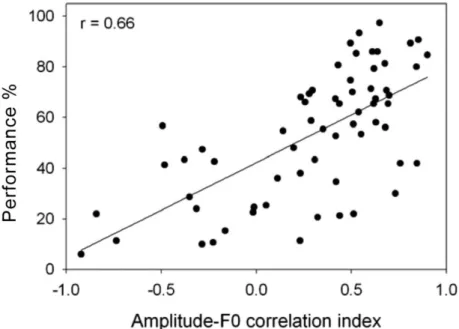
To explain the complex pattern of the effects of stimulus harmonics, a linear regression used between tone identification scores averaged over the ten listeners and the amplitude-F0 contour index for vocoded speech across the quiet and noisy conditions, following Fu and Zeng.[41] The amplitude-F0 contour index was calculated as the correlation between the F0 contour of the corresponding harmonic signal and the amplitude contour of a vocoded stimulus.

Figure 4.2: Linear regression function of average tone identification scores over the ten listeners vs. amplitude-F0 correlation index (Pearson r¼0.66, p<0.01).

(57)

46

As shown in Figure 4.2, there was a significant correlation between tone accuracy and the amplitude-F0 correlation index for vocoded speech, implying that as the amplitude contours were closer to the F0 contour, tone identification scores were raised.

4-1-4- Discussion

The purpose of this study was to investigate the contribution of low-frequency harmonics to Mandarin tone identification in vocoded speech simulating CI processing. Overall, the effects of low-frequency harmonics on tone identification were complicated, depending on the other four factors. For natural speech presented in quiet and noisy conditions of a 10 dB SNR, the three low harmonics of both male and female speakers led to high tone identification accuracy (>90%), except H1 of the male speaker in noisy condition. The result of this condition might be due to relatively low audibility at the low-frequency (H1) of the male speaker (e.g., ~161 Hz). For vocoded speech in a quiet condition, tone identification with the three low harmonics was comparable to that with all harmonics, with average scores reaching about 60%–70%. However, for vocoded speech in noise, average tone identification over the talkers and tone categories was reduced to 30%–40% and was better for all harmonics than for individual harmonics, especially H1. It should also be mentioned that the contribution of low-frequency harmonics changed with the tone categories for vocoded speech. For instance, for tones 1, 2, and 3, the stimuli with all harmonics had better or similar tone identification compared with the stimuli with individual harmonics, whereas for tone 4, the stimuli with all harmonics had substantially lower tone accuracy than those with individual harmonics. As shown in Figure 4.2, the complicated pattern of tone identification for the vocoded speech was partially considered by the amplitude-F0 contour index. Furthermore, tone identification was significantly better for tone 3 and tone 4 than

(58)

47

for tone 1 and tone 2, especially for vocoded speech in quiet, consistent with previous reports. [40]

These results designate that the frequency contour of F0 and its harmonics played a dominating role in determining tone identification in quiet and in relatively high-SNR conditions, even though the frequency contour and amplitude contour of natural speech sometimes were not well correlated (e.g., the low amplitude-F0 contour index for tone 4). In a natural speech with phonation, frequency contours of low-frequency harmonics appeared to coincide with F0 contours such that high tone accuracy is reached. However, when low harmonics like H1 were not well audible in noise, tone identification was significantly reduced for tones 1, 2, and 3 of the male speaker (see the left-lower panel of Figure 4.1(b)). Interestingly, the identification score of tone 4 for the male H1 was quite high (96%), also possibly due to the relatively better audibility of the male H1 for tone 4 (e.g., the frequency ranged from 224 to 109 Hz). On the other hand, for vocoded speech, which removed F0 and tonal duration cues in the present study, listeners appeared to rely on temporal envelope cues like amplitude contour to identify tones [41], although tone identification was significantly degraded. Moreover, tone identification of vocoded speech was significantly lower in noise than in quiet, partially due to the disruption of the amplitude contour of speech signals by noise.

The effect of amplitude contour on tone identification seemed to be frequency independent. That is, regardless of broad frequency ranges for the stimuli with all harmonics or narrow low-frequency ranges for the individual harmonics. Tone identity was significantly connected with the amplitude contour of the stimulus. For example, tone 4 had significantly lower identification scores for the stimulus with all harmonics than for stimuli with individual harmonics, mainly because the amplitude contour was slightly rising or flat for the stimulus with