Optimal Monetary Policy in an Operational Medium-Sized DSGE Model

NBER WORKING PAPER SERIES

OPTIMAL MONETARY POLICY IN AN OPERATIONAL MEDIUM-SIZED DSGE

MODEL

Malin Adolfson

Stefan Laséen

Jesper Lindé

Lars E.O. Svensson

Working Paper 14092

http://www.nber.org/papers/w14092

NATIONAL BUREAU OF ECONOMIC RESEARCH

1050 Massachusetts Avenue

Cambridge, MA 02138

June 2008

We are grateful for helpful comments from Günter Coenen, Lee Ohanian, Frank Smets, and participants

in the Second Oslo Workshop on Monetary Policy, the Central Bank Workshop on Macroeconomic

Modelling, Oslo, the conference on New Perspectives on Monetary Policy Design, Barcelona, the

Lindahl Lectures, Uppsala, the conference on Quantitative Approaches to Monetary Policy in Open

Economies, Atlanta, and seminars at the Riksbank and the Institute for International Economic Studies.

All remaining errors are ours. The views, analysis, and conclusions in this paper are solely the responsibility

of the authors and do not necessarily agree with those of other members of the Riksbank’s staff or

executive board, the Federal Reserve Board, or the National Bureau of Economic Research.

NBER working papers are circulated for discussion and comment purposes. They have not been

peer-reviewed or been subject to the review by the NBER Board of Directors that accompanies official

NBER publications.

© 2008 by Malin Adolfson, Stefan Laséen, Jesper Lindé, and Lars E.O. Svensson. All rights reserved.

Short sections of text, not to exceed two paragraphs, may be quoted without explicit permission provided

Optimal Monetary Policy in an Operational Medium-Sized DSGE Model

Malin Adolfson, Stefan Laséen, Jesper Lindé, and Lars E.O. Svensson

NBER Working Paper No. 14092

June 2008, Revised December 2010

JEL No. E52,E58,F41

ABSTRACT

We show how to construct optimal policy projections in Ramses, the Riksbank’s open-economy medium-sized

DSGE model for forecasting and policy analysis. Bayesian estimation of the parameters of the model

indicates that they are relatively invariant to alternative policy assumptions and supports our view

that the model parameters may be regarded as unaffected by the monetary policy specification. We

discuss how monetary policy, and in particular the choice of output gap measure, affects the transmission

of shocks. Finally, we use the model to assess the recent Great Recession in the world economy and

how its impact on the economic development in Sweden depends on the conduct of monetary policy.

This provides an illustration on how Rames incorporates large international spillover effects.

Malin Adolfson

Sveriges Riksbank

SE-103 37 Stockholm

Sweden

[email protected]

Stefan Laséen

Sveriges Riksbank

SE-103 37 Stockholm

Sweden

[email protected]

Jesper Lindé

International Finance

Mail Stop 20

Federal Reserve Board

20th and C streets, NW

Washington, D.C. 20551

[email protected]

Lars E.O. Svensson

Sveriges Riksbank

SE-103 37 Stockholm

SWEDEN

and Sveriges Riksbank

and also NBER

Contents

1 Introduction . . . 1

2 The model . . . 3

2.1 Domestic goodsfirms . . . 4

2.2 Importing and exporting firms . . . 5

2.3 Households . . . 6

2.4 Structural shocks, government, foreign economy . . . 8

2.5 Monetary policy . . . 9

2.6 Model solution . . . 11

3 Estimation . . . 12

3.1 Data, prior distributions, and calibrated parameters . . . 12

3.2 Estimation results . . . 14

4 Monetary policy and the transmission of shocks . . . 17

5 Optimal policy projections and the Great Recession . . . 20

5.1 Information and data . . . 20

5.2 The projection model and optimal projections . . . 21

5.3 An application to the Great Recession . . . 23

6 Conclusions . . . 28

Appendix . . . 29

A Ramses in some detail . . . 29

B Optimal projections in some detail . . . 34

B.1 Information and data . . . 34

B.2 Solving for the optimal projection . . . 35

B.3 Determination of the initial Lagrange multipliers . . . 36

B.4 Projections with an arbitrary instrument rule . . . 37

C Flexprice equilibrium and alternative concepts of potential output . . . 38

C.1 Unconditional potential output . . . 40

C.2 Conditional potential output . . . 40

C.3 Projections of potential output . . . 41

1. Introduction

We study optimal monetary policy in Ramses, the main model used at Sveriges Riksbank for forecasting and policy analysis. Ramses is an estimated small open-economy dynamic stochastic general equilibrium (DSGE) model, developed by Adolfson, Laséen, Lindé, and Villani (ALLV) [4] and [3].

By optimal monetary policy we mean policy that minimizes an intertemporal loss function. The intertemporal loss function is a discounted sum of expected future period losses. We choose a quadratic period loss function that corresponds to flexible inflation targeting and is the weighted sum of three terms: the squared inflation gap between 4-quarter CPI inflation and the inflation target, the squared output gap between output and potential output, and the squared quarterly change in the Riksbank’s instrument rate, the repo rate. We interpret such a loss function as con-sistent withflexible inflation targeting and the Riksbank’s mandate, which implies that monetary policy is directed towards stabilizing both inflation around an inflation target of 2 percent and resource utilization around a normal level ([36]).1

A fundamental assumption in our analysis is that Ramses is a structural model whose parameters are invariant to the changes in monetary policy we consider. We estimate the model parameters with Bayesian techniques under different assumptions about the conduct of monetary policy. First, as in ALLV [3], we estimate the model under the assumption that the Riksbank has followed a simple instrument rule during the inflation-targeting period which started in 1993:1.2 Second, we estimate the model under the assumption that the Riksbank has minimized an intertemporal loss function during the inflation-targeting period. The estimates of the instrument-rule and loss-function parameters provide benchmarks for the subsequent policy analysis. A finding in the empirical analysis is that whether past policy of the Riksbank until 2007:3 (the end of the sample used) is better explained as following a simple instrument rule or minimizing a loss function depends on whether the simple instrument rule and the optimal policy rule has a white-noise policy shock (control error) or not. Without a shock in both rules, we find that optimal policy fits the data

1

In some simple models, quadratic approximations of the welfare of a representative household results in a similar period loss function (Woodford [38]). Such approximations of household welfare are very model-dependent and reflect the particular distortions assumed in any given model. Household welfare is in any case hardly an operational central-bank objective, although it may be of interest and relevant to examine how household welfare in particular models is affected by central-bank policy. Such an undertaking is beyond the scope of the present paper, though.

2

The inflation-targeting period is assumed to start 1993:1 (the estimation sample in this paper ends 2007:3). Prior to this period (1986:1—1992:4), the conduct of policy is assumed to be given by a simple instrument rule. The switch to the inflation-targeting regime in 1993:1 is assumed to be completely unanticipated but expected to be permanent once it has occurred.

equally well as the simple instrument rule. With a shock in both rules, there is a clear improvement in the empirical fit of both rules. Furthermore, the simple instrument rule has a slight empirical advantage relative to optimal policy. Hence, for the particular sample period in question, with policy shocks the simple instrument rule offers a slightly better characterization of monetary policy. Our results are hence slightly different than those reported by Wolden Bache, Brubakk, and Maih [37] on Norwegian data, which stems from the fact that they do not allow for a control error in their analysis.

One contribution of our paper is to provide a detailed analysis of how to do optimal policy projections in an estimated linear-quadratic model with forward-looking variables, extending on previous analysis by Svensson [28] and Svensson and Tetlow [34]. A key issue for aflexible inflation-targeting central bank is which measure of resource utilization to stabilize. We use the output gap as measure of resource utilization and study alternative definitions of potential output and the output gap, in order to make an assessment to what extent the formulation of the output gap in the loss function affects the conduct of monetary policy and propagation of shocks. More precisely, we report results from three alternative concepts of output gaps (−¯), deviations of actual (log) output ()

from potential (log) output (¯), in the loss function. One concept of output gap is thetrend output

gap where potential output is the trend output level, which is growing stochastically due to the unit-root stochastic technology shock in the model. A second concept is theunconditional output gap, where potential output is unconditional potential output, which is defined as the hypothetical output level that would exist if the economy would have hadflexible prices and wages for a long time and would have been subject to a subset of the same shocks as the actual economy. Unconditional potential output therefore presumes different levels of the predetermined variables, including the capital stock, from those in the actual economy. A third concept is the conditional output gap, where potential output is conditional potential output, which is defined as the hypothetical output level that would arise if prices and wages suddenly become flexible in the current period and are expected to remain flexible in the future. Conditional potential output therefore depends on the existing current predetermined variables, including the current capital stock.

To illustrate how the policy maker’s choice of output measure can influence the transmission of shocks we study impulse response functions to a persistent but stationary technology shock. Ac-cording to the estimated model, shocks to total factor productivity is a dominant driver of business cycles in Sweden. In addition to its economic importance, this shock is also particularly interesting to study since it affects the various output gaps differently. Conditional and unconditional

poten-tial output increases when a positive stationary technology shock hits the economy, whereas trend output by definition is independent of such shocks and only depends on permanent (unit-root) technology shocks.

With that analysis in hand, we report and discuss optimal policy projections for Sweden using data up to and including 2008:2. We use the model to interpret the economic development in Sweden just at the time when the world economy fell into a deep recession due to the collapse in thefinancial markets. We choose this period to highlight the sensitivity of the Swedish economy to foreign shocks. We show projections for the estimated instrument rule and for optimal policy with different output gaps in the loss function, which create different trade-offs for the central bank in stabilizing inflation and output.

The paper is organized as follows: Section 2 presents Ramses in more general modeling terms. Section 3 discusses the data and priors used in the estimation and presents estimation results for the various specifications of the model and policy. Section 4 presents and discusses impulse response functions to a technology shock with different output gaps in the loss function. Section 5 discusses how to construct optimal policy projections, and analyzes alternative projections for a policymaker during the recent Great Recession. Finally, section 6 presents a summary and some conclusions. Appendices A-B contain a detailed specification of Ramses and some other technical details.

2. The model

Ramses is a small open-economy DSGE model developed in a series of papers by ALLV [4] and [3]. The model economy consists of households, domestic goodsfirms, importing consumption and importing investmentfirms, exportingfirms, a government, a central bank, and an exogenous foreign economy. Within each manufacturing sector there is a continuum of firms that each produces a differentiated good and sets prices according to an indexation variant of the Calvo model. Domestic as well as global production grows with technology that contains a stochastic unit-root, see Altig et al. [8].

In what follows we provide the optimization problems of the differentfirms and the households, and describe the behavior of the central bank. The log-linear approximation of the model is presented in appendix A.

2.1. Domestic goods firms

The domestic goods firms produce their goods using capital and labor inputs, and sell them to a retailer which transforms the intermediate products into a homogenous final good that in turn is sold to the households.

The final domestic good is a composite of a continuum of differentiated intermediate goods, each supplied by a different firm. Output, , of the final domestic good is produced with the

constant elasticity of substitution (CES) function

= ⎡ ⎣ 1 Z 0 () 1 _{ } ⎤ ⎦    1_≤_ _∞ (2.1)

where , 0 ≤  ≤ 1, is the input of intermediate good  and  is a stochastic process that

determines the time-varyingflexible-price markup in the domestic goods market. The production of the intermediate good by intermediate-good firmis given by

=1−1−− (2.2)

where is a unit-root technology shock common to the domestic and foreign economies,is a

do-mestic covariance stationary technology shock, the capital stock and denotes homogeneous

labor hired by the  firm. A fixed cost  is included in the production function. We set this

parameter so that profits are zero in steady state, following Christiano et al. [11].

We allow for working capital by assuming that a fraction  of the intermediate firms’ wage bill has to befinanced in advance through loans from a financial intermediary. Cost minimization yields the following nominal marginal cost for intermediatefirm:

MC_= 1 (1₋)1− 1 (  )[(1 +(−1−1))]1− 1 1− 1   (2.3)

where _ is the gross nominal rental rate per unit of capital, −1 the gross nominal (economy

wide) interest rate, and the nominal wage rate per unit of aggregate, homogeneous, labor.

Each of the domestic goods firms is subject to price stickiness through an indexation variant of the Calvo [10] model. Each intermediate firm faces in any period a probability 1₋_ that it can reoptimize its price. The reoptimized price is denoted _. For the firms that are not allowed to reoptimize their price, we adopt an indexation scheme with partial indexation to the current inflation target, ¯_+1, since there is a perceived (time-varying) CPI inflation target in the model ,

and partial indexation to last period’s inflation rate in order to allow for a lagged pricing term in the Phillips curve

_₊₁=³_´¡¯_+1¢1−

_ (2.4)

where _ is the price level, _ = _₊₁_ is gross inflation in the domestic sector, and  is an

indexation parameter. The different firms maximize profits taking into account that there might not be a chance to optimally change the price in the future. Firm  therefore faces the following optimization problem when setting its price

max _ E ∞ P =0 (_)+[(¡+1+−1 ¢¡ ¯ _₊₁¯_+2¯_+¢1− _)+ −MC_{+}(+++)] (2.5)

where the firm is using the stochastic household discount factor (_)+ to make profits

con-ditional upon utility  is the discount factor, and + the marginal utility of the households’

nominal income in period+, which is exogenous to the intermediatefirms. 2.2. Importing and exporting firms

The importing consumption and importing investment firms buy a homogenous good at price _∗ in the world market, and convert it into a differentiated good through a brand naming technology. The exporting firms buy the (homogenous) domestic final good at price _ and turn this into a differentiated export good through the same type of brand naming. The nominal marginal cost of the importing and exporting firms are thus ∗ and , respectively, where  is the

nominal exchange rate (domestic currency per unit of foreign currency). The differentiated import and export goods are subsequently aggregated by an import consumption, import investment and export packer, respectively, so that the final import consumption, import investment, and export good is each a CES composite according to the following:

_= ⎡ ⎣ 1 Z 0 (_) 1 _{ } ⎤ ⎦    _ = ⎡ ⎣ 1 Z 0 (_) 1 _{ } ⎤ ⎦   = ⎡ ⎣ 1 Z 0 () 1 _{ } ⎤ ⎦   (2.6) where 1 _≤ 

  ∞ for  = {  } is the time-varying flexible-price markup in the import

consumption (), import investment () and export () sector. By assumption the continuum of consumption and investment importers invoice in the domestic currency and exporters in the foreign currency. To allow for short-run incomplete exchange rate pass-through to import as well as export prices we introduce nominal rigidities in the local currency price. This is modeled through

the same type of Calvo setup as above. The price setting problems of the importing and exporting firms are completely analogous to that of the domestic firms in equation (2.5).3 In total there are thus four specific Phillips curve relations determining inflation in the domestic, import consumption, import investment and export sectors.

2.3. Households

There is a continuum of households which attain utility from consumption, leisure and real cash balances. The preferences of household  are given by

E₀ ∞ X =0  ⎡ ⎢ ⎣_ln (−−1)− ()1+ 1 + + ³_   ´ 1₋ 1−⎤ ⎥ ⎦ (2.7)

where,anddenote thehousehold’s levels of aggregate consumption, labor supply

and real cash holdings, respectively. Consumption is subject to habit formation through −1,

such that the household’s marginal utility of consumption is increasing in the quantity of goods consumed last period. _ and_ are persistent preference shocks to consumption and labor supply, respectively. Households consume a basket of domestically produced goods (_) and imported products (_) which are supplied by the domestic and importing consumptionfirms, respectively. Aggregate consumption is assumed to be given by the following CES function:

= h (1₋)1_( )(−1)+ 1  () (−1) i(−1) 

where  is the share of imports in consumption, and  is the elasticity of substitution across

consumption goods.

The households can invest in their stock of capital, save in domestic bonds and/or foreign bonds and hold cash. The households invest in a basket of domestic and imported investment goods to form the capital stock, and decide how much capital to rent to the domestic firms given costs of adjusting the investment rate. The households can increase their capital stock by investing in additional physical capital (), taking one period to come in action. The capital accumulation

equation is given by

+1= (1−)+Υ[1−˜(−1)] (2.8)

3

Total export demand satisfies  +   = _  ∗  −_ ∗, where    and  

 is demand for consumption and investment goods, respectively;

 the export price;∗the foreign price level;∗foreign output and the elasticity of substitution across foreign goods

where ˜(−1) determines the investment adjustment costs through the estimated parameter

˜

00, andΥis a stationary investment-specific technology shock. Total investment is assumed to be

given by a CES aggregate of domestic and imported investment goods (_ and _, respectively) according to = ∙ (1₋)1 ³ _´(−1)+1  (   )(−1) ¸(−1)  (2.9)

where  is the share of imports in investment, and  is the elasticity of substitution across

investment goods.

Each household is a monopoly supplier of a differentiated labor service which implies that they can set their own wage, see Erceg, Henderson and Levin [15]. After having set their wage, households supply thefirms’ demand for labor,

 = ∙   ¸  1− 

at the going wage rate. Each household sells its labor to afirm which transforms household labor into a homogenous good that is demanded by each of the domestic goods producing firms. Wage stickiness is introduced through the Calvo [10] setup, where household  reoptimizes its nominal wage rate_ according to the following4

max   EP∞_=0()  [₋_+(+) 1+_ 1+ + +( 1−_+) (1+ +) ³¡ __+−1¢¡ ¯ _+1¯__+¢(1−)¡ _+1_{+}¢_´+] (2.10)

where_is the probability that a household is not allowed to reoptimize its wage,_ a labor income tax,_ a pay-roll tax (paid for simplicity by the households), and _=−1 is the growth rate

of the unit-root technology shock.

The choice between domestic and foreign bond holdings balances into an arbitrage condition pinning down expected exchange rate changes (that is, an uncovered interest rate parity condition). To ensure a well-defined steady-state in the model, we assume that there is premium on the foreign bond holdings which depends on the aggregate net foreign asset position of the domestic households, see, for instance, Schmitt-Grohé and Uribe [23]. Compared to a standard setting the risk premium is allowed to be negatively correlated with the expected change in the exchange rate (that is, the expected depreciation), following the evidence discussed in for example Duarte and Stockman [14].

4

For the households that are not allowed to reoptimize, the indexation scheme is +1 = (

)

_(¯_+1)(1−)_

For a detailed discussion and evaluation of this modification see ALLV [3]. The risk premium is given by: Φ( ˜) = exp µ −˜_(−¯)−˜ µ +1   −1 − 1 ¶ + ˜_ ¶  (2.11)

where≡(∗)() is the net foreign asset position, and˜ is a shock to the risk premium.

To clear the final goods market, the foreign bond market, and the loan market for working capital, the following three constraints must hold in equilibrium:

_+_+++ ≤1−1−− (2.12)

∗+1=(+)−∗(+) +∗−1Φ(−1e−1)∗ (2.13)

=− (2.14)

where  is government expenditures,  and  are the foreign demand for export goods which

follow CES aggregates with elasticity _, and _ = +1 is the monetary injection by the

central bank. When defining the demand for export goods, we introduce a stationary asymmetric (or foreign) technology shock ˜∗

 = ∗, where ∗ is the permanent technology level abroad, to

allow for temporary differences in permanent technological progress domestically and abroad. 2.4. Structural shocks, government, foreign economy

The structural shock processes in the model are given by the univariate representation

ˆ

=ˆ−1+  

∼ ¡0 2_¢ (2.15) where  = { ,     Υ ˜ ¯ ˜∗},  = {   } and a hat denotes the

deviation of a log-linearized variable from a steady-state level (ˆ≡for any variable, where

 is the steady-state level). _ and  are assumed to be white noise (that is, = 0 _

 = 0).

The government spends resources on consuming part of the domestic good, and collects taxes from the households. The resulting fiscal surplus/deficit plus the seigniorage are assumed to be transferred back to the households in a lump sum fashion. Consequently, there is no government debt. The fiscal policy variables — taxes on labor income (ˆ_), consumption (ˆ_), and the pay-roll (ˆ_), together with (HP-detrended) government expenditures (ˆ) — are assumed to follow an

identified VAR model with two lags,

where  ≡(ˆˆˆˆ)0,   ∼ (0 ),  is a diagonal matrix with standard deviations and

Θ−₀1 ∼(0Σ).

Since Sweden is a small open economy we assume that the foreign economy is exogenous. Foreign inflation, ∗_, output (HP-detrended), ˆ_∗ and interest rate,∗_, are exogenously given by an identified VAR model with four lags,

Φ0∗=Φ1∗−1+Φ2∗−2+Φ3∗−3+Φ4∗−4+∗∗ (2.17)

where _∗ _≡ (_∗ˆ∗_ ∗_)0, ∗ ∼ (0 ∗) ∗ is a diagonal matrix with standard deviations

and Φ−₀1∗_∗_ ∼ (0Σ_∗). Given our assumption of equal substitution elasticities in foreign

consumption and investment, these three variables suffice to describe the foreign economy in our model setup.

2.5. Monetary policy

Monetary policy is modeled in two different ways. First, we assume that the central bank minimizes an intertemporal loss function under commitment. Let the intertemporal loss function in period  be E ∞ X =0 + (2.18)

where0  1 is a discount factor, is the period loss that is given by

= (−−4−¯)2+(−¯)2+∆(−−1)2 (2.19)

where the central bank’s target variables are; model-consistent year-over-year CPI inflation rate, _{ −}_−4, where _ denotes the log of CPI and ¯ is the 2 percent inflation target; a measure of the output gap, −¯; thefirst difference of the instrument rate, −−1, where  denotes the

Riksbank’s instrument rate, the repo rate, and and∆ are nonnegative weights on output-gap

stabilization and instrument-rate smoothing, respectively.5

We report results from three alternative concepts of output gaps (−¯) as measures of resource

utilization in the loss function. One concept of output gap is thetrend output gap where potential output (¯) is the trend output level, which is growing stochastically due to the unit-root stochastic

technology shock in the model. A second concept is theunconditional output gap, where potential output is unconditional potential output, which is defined as the hypothetical output level that

5

We use the 4-quarter CPI difference as a target variable rather than quarterly inflation since the Riksbank and other inflation-targeting central banks normally specify their inflation target as a 12-month rate.

would exist if the economy would have had flexible prices and wages for a long time and would have been subject to the same shocks as the actual economy except mark-up shocks and shocks to taxes which are held constant at their steady-state levels. Unconditional potential output therefore presumes different levels of the predetermined variables, including the capital stock, from those in the actual economy. A third concept is the conditional output gap, where potential output is conditional potential output, which is defined as the hypothetical output level that would arise if prices and wages suddenly becomeflexible in the current period and are expected to remainflexible in the future. Conditional potential output therefore depends on the existing current predetermined variables, including the current capital stock. In precise form the three different concepts ofpotential

output are ¯ trend_ = ¯ _cond=__· ¯ uncond_ =__·_

where  is the unit-root technology shock, the row vector · expresses output as a function of

the predetermined state variables in theflex-price economy,is the vector of predetermined state

variables in Ramses, and _ is the state vector in the economy with flexible prices and wages. Second, we assume that monetary policy obeys an instrument rule, following Smets and Wouters [25]. Instead of optimizing an intertemporal loss function, the central bank is then assumed to adjust the short term interest rate in response to deviations of CPI inflation from the perceived inflation target, the trend output gap (measured as actual minus trend output), the real exchange rate

(ˆ≡ˆ+ ˆ∗−ˆ)and the interest rate set in the previous period. The log-linearized instrument

rule follows:  = −1+ (1−) h b¯ _+ ¡ ˆ _−1−b¯_¢+ˆ−1+b˜−1 i (2.20) +∆ ¡ ˆ _−ˆ_−1¢+∆(ˆ−ˆ−1) +

where  ≡ˆ (the notation for the short nominal interest rate in Ramses), and  is an

uncor-related monetary policy shock. Since ˆ_ and ˆ are forward-looking variables, this is an implicit

instrument rule (see appendix B.4).6 6

As reported in ALLV [3], the output gap resulting from trend output seems to more closely correspond to the measure of resource utilization that the Riksbank has been responding to historically rather than the unconditional output gap. Del Negro, Schorfheide, Smets, and Wouters [13] report similar results for the US.

2.6. Model solution

After log-linearization, Ramses can be written in the following state-space form, ∙ +1 +1| ¸ = ∙   ¸ ++ ∙  0 ¸ +1 (2.21)

Here,  is an -vector of predetermined variables in period  (where the period is a quarter);

 is an -vector of forward-looking variables;  is an -vector of instruments (the

forward-looking variables and the instruments are the nonpredetermined variables);7  is an -vector of

i.i.d. shocks with mean zero and covariance matrix ; , , and , and  are matrices of the

appropriate dimension; and, for any variable , +| denotesE+, the rational expectation of

+ conditional on information available in period . The variables are measured as differences

from steady-state values; thus their unconditional means are zero. The elements of the matrices ,,, and  are estimated with Bayesian methods and are considered fixed and known for the policy simulations. Then the conditions for certainty equivalence are satisfied. Thus, we abstract from any consideration of model uncertainty in the formulation of optimal policy.8

The upper block of (2.21) provides  equations that determine the-vector +1 in period

+ 1for given,,and +1

+1=11+12+1++1 (2.22)

where and  are partitioned conformably with and as

_≡ ∙ 11 12 21 22 ¸  = ∙ 1 2 ¸  (2.23)

The lower block provides equations that determine the -vector in period for given+1|,

, and 

=−221(+1|−21−2) (2.24)

We hence assume that the × submatrix 22 is nonsingular.9

We assume that the central bank’s -vector of target variables, measured as the difference

from an -vector ∗ of target levels ≡ (−−4−¯ −¯ −−1)0, can be written as a

7 _{A variable is predetermined if its one-period-ahead prediction error is an exogenous stochastic process (Klein}

[20]). For (2.21), the one-period-ahead prediction error of the predetermined variables is the stochastic vector+1.

8

Onatski and Williams [22] provide a thorough discussion of model uncertainty. Svensson and Williams [32] and [33] show how to compute optimal policies for Markov Jump-Linear-Quadratic systems, which provide a quiteflexible way to model most kinds of relevant model uncertainty for monetary policy. Levin, Onatski, Williams and Williams [19] study optimal policy when the central bank faces uncertainty about the true structure of the economy (i.e., they look at the entire posterior distribution of the model parameters).

9

Without loss of generality, we assume that the shocksonly enter in the upper block of (2.21), since any shocks in the lower block of (2.21) can be redefined as additional predetermined variables and introduced in the upper block.

linear function of the predetermined, forward-looking, and instrument variables, = ⎡ ⎣    ⎤ ⎦_≡[  ] ⎡ ⎣    ⎤ ⎦ (2.25)

whereis an×(++)matrix and partitioned conformably with,, and. Assuming

optimization of (2.18) under commitment in a timeless perspective, the resulting intertemporal equilibrium can then be described by the following difference equations,

∙   ¸ =  ∙  Ξ−1 ¸  (2.26) ∙ +1 Ξ ¸ =  ∙  Ξ−1 ¸ + ∙  0 ¸ +1 (2.27)

for  _≥ 0, where 0 and Ξ−1 are given. This system of difference equations can be solved with

several alternative algorithms, for instance those developed by Klein [20] and Sims [24].10 The choice and calculation of the initialΞ₋1 is further discussed in footnote 14 and appendix B.3.

When policy instead is described by the simple instrument rule in (2.20), there exists  and  matrices such that the intertemporal equilibrium difference equations (2.26) and (2.27) are still valid but with Ξ= 0for ≥0.

3. Estimation

3.1. Data, prior distributions, and calibrated parameters

We use quarterly Swedish data for the period 1980:1-2007:3 and estimate the model using a Bayesian approach by placing a prior distribution on the structural parameters.1112

As in ALLV [3], we include the following  = 15 variables among the observable variables:

GDP deflator inflation (_), real wage (), consumption (), investment (), real exchange

rate (˜), short interest rate (), hours worked (), GDP (), exports (˜), imports (˜), CPI

inflation (cpi_ ), investment-deflator inflation (def_ ), foreign (trade-weighted) output (_∗), foreign inflation (∗_), and foreign interest rate (∗_). We usefirst differences of the quantities and the real

1 0 _{See Svensson [28] and [29] for details of the derivation and the application of the Klein algorithm.}

1 1 _{All data are from Statistics Sweden, except the repo rate which is from the Riksbank. The nominal wage is}

deflated by the GDP deflator. Foreign inflation, output, and interest rate are weighted together across Sweden’s 20 largest trading partners in 1991 using weights from the IMF.

1 2

In the data, the ratios of import and export to output are increasing from about 025to 040and from021 to050, respectively, during the sample period. In the model, import and export are assumed to grow at the same rate as output. We have removed the excess trend in import and export in the data to make the export and import shares stationary. For all other variables we use the actual series (seasonally adjusted with the X12-method, except the variables in the GDP identity which were seasonally adjusted by Statistics Sweden).

wage, since the unit-root technology shock induces a common stochastic trend in these variables, and derive the state-space representation for the following vector of observed variables,

≡ (_∆ln()∆ln∆lnb˜ ˆ  ∆ln∆ln ˜∆ln ˜ cpi   def  ∆ln∗ ∗ ∗)0 (3.1) The growth rates are computed as quarterly log-differences, while the inflation and interest-rate series are measured as annualized quarterly rates. It should be noted that the stationary variables

b˜

 and ˆ are measured as deviations around the mean and the HP-filtered trend, that is, b˜ ≡ (˜−˜)˜ andˆ≡

¡

−HP

¢

HP

 , respectively.13 Finally, all real variables are measured in

per-capita units.

We estimate 13 structural shocks, of which 8 follow AR(1) processes and 5 are assumed to be i.i.d. (as described in section 2.4). In addition to these, there are 8 shocks provided by the exogenous (pre-estimated) fiscal and foreign VARs, whose parameters are kept fixed throughout the estimation of the model (uninformative priors are used for these stochastic processes). The shocks enter in such a way that there is no stochastic singularity in the likelihood function.

To compute the likelihood function, the reduced-form solution of the model (2.26-2.27) is trans-formed into a state-space representation that maps the unobserved state variables into the observed data.14 The posterior mode and Hessian matrix evaluated at the mode is computed by standard numerical optimization routines (see Smets and Wouters [25] and the references there for details). The parameters we choose to estimate pertain mostly to the nominal and real frictions in the model and the exogenous shock processes.15 Table 3.1 shows the assumptions for the prior distribution of the estimated parameters. For the model with a simple instrument rule, we choose identical priors for the parameters in the instrument rule before and after the adoption of an

1 3

The reason why we use a smooth HP-filtered trend for hours per capita, as opposed to a constant mean, is that there is a large and very persistent reduction in hours worked per capita during the recession in the beginning of the 1990s. Neglecting taking this reduction into account implies that the forecasting performance for hours per capita in the model deteriorates significantly, as documented in the forecasting exercises in ALLV [3]. Rather than imposing a discrete shift in hours in a specific time period, we therefore decided to remove a smooth HP trend from the variable. This choice is not particularly important for the parameter estimates, but has some impact on the 2-sided filtered estimates of the unobserved states of the economy.

1 4 _{We use the Kalman filter to calculate the likelihood function of the observed variables. The period 1980:1—}

1985:4 is used to form a prior on the unobserved state variables in 1985:4, and the period 1986:1-2007:3 is used for inference. During estimation the Lagrange multipliers,Ξare updated through the Kalman filter just as the other state variables. When the instrument rule is activeΞequals zero, and in 1993:1, when policy (unexpectedly) switches to minimizing the loss function, we assume commmitment from scratch so that the initial Lagrange multipliers are zero.

1 5 _{We choose to calibrate those parameters that we think are weakly identified by the variables that we include in}

the vector of observed data. These parameters are mostly related to the steady-state values of the observed variables (that is, the great ratios: , , and). The parameters that we calibrate are set as follows: the money growth= 1010445; the discount factor= 0999999; the steady state growth rate of productivity_= 1005455; the depreciation rate˜= 0025; the capital share in production= 025; the share of imports in consumption and investment= 035and= 050, respectively; the share of wage billfinanced by loans= 1; the labour supply elasticity= 1; the wage markup= 130; inflation target persistence= 0975; the steady-state tax rates on labour income and consumption= 030and= 024, respectively; government expenditures-output ratio 030; and the subsitution elasticity between consumption goods_= 5.

inflation target in 1993:1. For the model with optimal policy during the inflation-targeting regime, we use very uninformative priors for the loss-function parameters ( and∆), as indicated by the

high standard deviations. As mentioned in the introduction, the switch from the simple instrument rule to the inflation-targeting regime in 1993:1 is modelled as unanticipated and expected to last forever once it has occurred.

Relative to other estimated small open-economy DSGE models (for instance, Justiniano and Preston [16]), the international spillover effects are relatively large due to the inclusion of a world-wide stochastic technology shock. This means that the open-economy aspects are of particular importance in our setting.

3.2. Estimation results

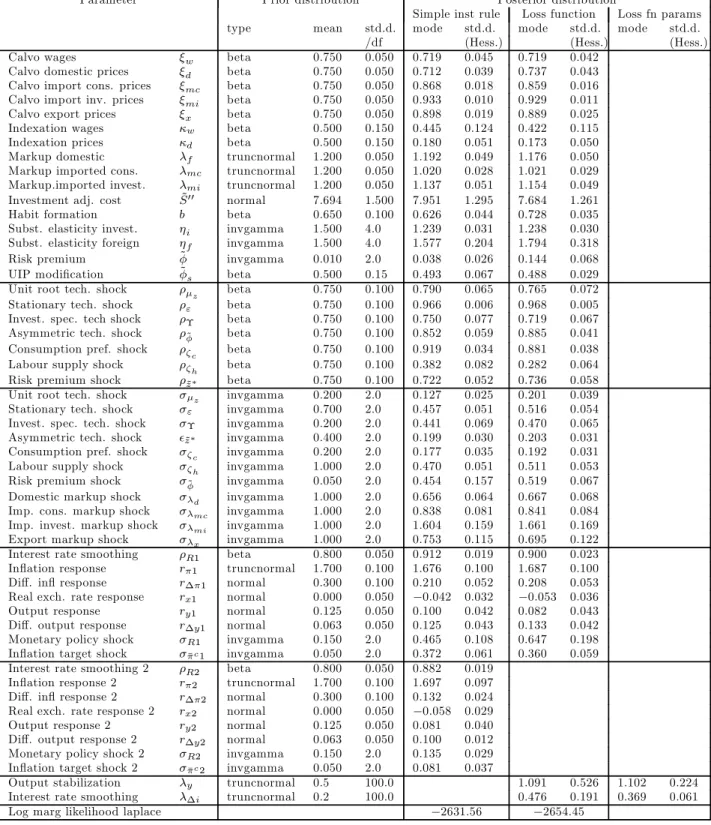
In table 3.1, we report the prior and estimated posterior distributions. Three posterior distributions are reported. The first, labeled “Simple inst rule”, is under the assumption that the Riksbank has followed a simple instrument rule during the inflation-targeting period (see equation (2.20)). The second, labeled “Loss function”, is under the assumption that the Riksbank has minimized a quadratic loss function under commitment during the inflation-targeting period, with the output gap in the loss function being the trend output gap (see equation (2.19)). In this case, the optimal policy rule does not include a policy shock. The third, labeled “Loss fn params”, only estimates the two parameters in that loss function.16

1 6 _{The estimations are based on allowing the inflation target to be time-varying. The parameter estimates are,}

Table 3.1: Prior and posterior distributions

Parameter Prior distribution Posterior distribution

Simple inst rule Loss function Loss fn params type mean std.d. mode std.d. mode std.d. mode std.d.

/df (Hess.) (Hess.) (Hess.)

Calvo wages  beta 0.750 0.050 0.719 0.045 0.719 0.042

Calvo domestic prices  beta 0.750 0.050 0.712 0.039 0.737 0.043

Calvo import cons. prices _ beta 0.750 0.050 0.868 0.018 0.859 0.016 Calvo import inv. prices _ beta 0.750 0.050 0.933 0.010 0.929 0.011 Calvo export prices  beta 0.750 0.050 0.898 0.019 0.889 0.025

Indexation wages  beta 0.500 0.150 0.445 0.124 0.422 0.115

Indexation prices  beta 0.500 0.150 0.180 0.051 0.173 0.050

Markup domestic  truncnormal 1.200 0.050 1.192 0.049 1.176 0.050

Markup imported cons.  truncnormal 1.200 0.050 1.020 0.028 1.021 0.029

Markup.imported invest.  truncnormal 1.200 0.050 1.137 0.051 1.154 0.049

Investment adj. cost ˜00 _{normal 7.694 1.500 7.951 1.295 7.684 1.261}

Habit formation  beta 0.650 0.100 0.626 0.044 0.728 0.035 Subst. elasticity invest. _ invgamma 1.500 4.0 1.239 0.031 1.238 0.030 Subst. elasticity foreign  invgamma 1.500 4.0 1.577 0.204 1.794 0.318

Risk premium ˜ invgamma 0.010 2.0 0.038 0.026 0.144 0.068 UIP modification ˜ beta 0.500 0.15 0.493 0.067 0.488 0.029

Unit root tech. shock _ beta 0.750 0.100 0.790 0.065 0.765 0.072

Stationary tech. shock _ beta 0.750 0.100 0.966 0.006 0.968 0.005 Invest. spec. tech shock Υ beta 0.750 0.100 0.750 0.077 0.719 0.067 Asymmetric tech. shock ˜ beta 0.750 0.100 0.852 0.059 0.885 0.041

Consumption pref. shock  beta 0.750 0.100 0.919 0.034 0.881 0.038 Labour supply shock _ beta 0.750 0.100 0.382 0.082 0.282 0.064

Risk premium shock ˜∗ beta 0.750 0.100 0.722 0.052 0.736 0.058

Unit root tech. shock _ invgamma 0.200 2.0 0.127 0.025 0.201 0.039

Stationary tech. shock  invgamma 0.700 2.0 0.457 0.051 0.516 0.054

Invest. spec. tech. shock Υ invgamma 0.200 2.0 0.441 0.069 0.470 0.065 Asymmetric tech. shock ˜∗ invgamma 0.400 2.0 0.199 0.030 0.203 0.031

Consumption pref. shock  invgamma 0.200 2.0 0.177 0.035 0.192 0.031 Labour supply shock _ invgamma 1.000 2.0 0.470 0.051 0.511 0.053

Risk premium shock ˜ invgamma 0.050 2.0 0.454 0.157 0.519 0.067

Domestic markup shock  invgamma 1.000 2.0 0.656 0.064 0.667 0.068 Imp. cons. markup shock  invgamma 1.000 2.0 0.838 0.081 0.841 0.084 Imp. invest. markup shock  invgamma 1.000 2.0 1.604 0.159 1.661 0.169 Export markup shock  invgamma 1.000 2.0 0.753 0.115 0.695 0.122 Interest rate smoothing 1 beta 0.800 0.050 0.912 0.019 0.900 0.023

Inflation response 1 truncnormal 1.700 0.100 1.676 0.100 1.687 0.100

Diff. inflresponse ∆1 normal 0.300 0.100 0.210 0.052 0.208 0.053

Real exch. rate response 1 normal 0.000 0.050 −0.042 0.032 −0.053 0.036

Output response 1 normal 0.125 0.050 0.100 0.042 0.082 0.043

Diff. output response ∆1 normal 0.063 0.050 0.125 0.043 0.133 0.042

Monetary policy shock 1 invgamma 0.150 2.0 0.465 0.108 0.647 0.198

Inflation target shock ¯1 invgamma 0.050 2.0 0.372 0.061 0.360 0.059

Interest rate smoothing 2 2 beta 0.800 0.050 0.882 0.019

Inflation response 2 2 truncnormal 1.700 0.100 1.697 0.097

Diff. inflresponse 2 ∆2 normal 0.300 0.100 0.132 0.024

Real exch. rate response 2 2 normal 0.000 0.050 −0.058 0.029

Output response 2 2 normal 0.125 0.050 0.081 0.040

Diff. output response 2 ∆2 normal 0.063 0.050 0.100 0.012

Monetary policy shock 2 2 invgamma 0.150 2.0 0.135 0.029

Inflation target shock 2 ¯2 invgamma 0.050 2.0 0.081 0.037

Output stabilization  truncnormal 0.5 100.0 1.091 0.526 1.102 0.224

Interest rate smoothing ∆ truncnormal 0.2 100.0 0.476 0.191 0.369 0.061

There are two important facts to note in the first two posterior distributions. First, it is clear that the version of the model where policy is characterized with the simple instrument rule with an exogenous policy shock is a better characterization of how the Riksbank has conducted monetary policy during the inflation-targeting period. The difference between log marginal likelihoods is almost 23 in favor of the model with the instrument rule compared to the model with optimal policy. In terms of Bayesian posterior odds, this is overwhelming evidence against the loss-function characterization of the Riksbank’s past policy behavior. However, this result crucially depends on the assumption that the simple instrument rule includes a policy shock (control error) and that the optimal policy rule does not. If we follow Wolden Bache, Brubakk, and Maih [37] and treat the two cases symmetrically by not including a policy shock in the simple rule during the inflation targeting period, that is, we impose 2 = 0, then the log marginal likelihood falls to −26545,

which is almost the same as for the optimal policy, implying that optimal policy fits the data equally well in this case. Alternatively, we can treat the two cases symmetrically by including a shock in the optimal policy rule. This improves the fit of optimal policy, but the log marginal likelihood (₋26368) is then still lower than the log marginal likelihood for the simple instrument rule with a policy shock in table 3.1. Hence, for the particular sample period in question, with policy shocks in both rules the simple instrument rule offers a slightly better characterization of monetary policy. Compared to optimal policy the Bayesian posterior odds speak clearly in favor of the simple instrument rule, but in practice we have seen that log marginal likelihood differences (Laplace approximation) of these magnitudes do not necessarily generate very large discrepancies in terms of the forecasting accuracy, see ALLV [3] and Adolfson, Lindé and Villani [7]. Thus, the improvement infit relative to optimal policy is moderate.

Second, perhaps more relevant for our purpose, the non-policy parameters of the model are fairly invariant to the specification of how monetary policy has been conducted during the inflation-targeting period. This is also true for the non-policy parameters of the model with the simple instrument rule without the policy shock.17

One way to assess the quantitative importance of the parameter differences between the instru-ment rule and the loss function (columns “Simple inst rule” and “Loss function”) is to calibrate all parameters except the coefficients in the loss function to the estimates obtained in the simple rule specification of the model, and then reestimate the coefficients in the loss function conditional on

1 7

It should be noted that data are informative about the parameters as the posteriors are often different, and more concentrated, than the prior distributions. Moreover, Adolfson and Lindé [6] use Monte Carlo methods to study identification in a very similar model, andfind that while a few parameters are weakly identified in small samples, all parameters are unbiased and consistent.

these parameters. If the loss function parameters are similar, we can conjecture that the differences in deep parameters are quantitatively unimportant. The result of this experiment is reported in the last column in table 3.1 labeled “Loss fn params”, and, as conjectured, the resulting loss func-tion parameters are very similar to the ones obtained when estimating all parameters jointly. We interpret this result as support for our assumption that the non-policy parameters are unaffected by the alternative assumptions about the conduct of monetary policy we consider below.

In the subsequent analysis we use the posterior-mode estimates of the non-policy parameters for the model with the simple instrument rule. In most cases, the model with the simple instrument rule is also used to generate the (partly) unobserved state variables. For consistency reasons, the associated estimated loss function parameters = 1102and∆= 0369are therefore used in the

analysis below.

4. Monetary policy and the transmission of shocks

According to the estimated model, shocks to total factor productivity play a dominant role in explaining business cycle variations in Sweden, as these shocks can explain the negative correlation between GDP growth and CPI inflation in our sample. In Adolfson, Laséen, Lindé and Svensson [2], we show that stationary technology shocks are the single most important driver of output fluctuations around trend. To interpret and understand the development of the Swedish economy, it is therefore of key importance to analyze and understand the effects of this type of technology shock.

To illustrate how optimal policy projections are affected by which output measure the central bank tries to stabilize we therefore start by looking at impulse response functions to a stationary technology shock. Although this type of technology shock () is estimated to be quite persistent

(_ = 0966) it does not affect trend output in the model (which by definition is only influenced by the permanent technology shock, _). In contrast, the output level under flexible prices and wages, flexprice potential output, increases with the shock. Abstracting from the policy response to the shock this means that the trend- andflexprice-output gaps, by definition, will behave quite differently following this shock.

Figure 4.1 shows impulse response functions to a positive (one-standard deviation) stationary technology shock under the instrument rule and under optimal policy with different output gaps. The plots show deviations from trend, where by trend we mean the steady state. Output thus equals the trend output gap. The real interest rate is defined as the instrument rate less

1-quarter-Figure 4.1: Impulse responses to a (one-standard deviation) stationary technology shock under optimal policy for different output gaps and under the instrument rule

0 10 20 −0.6 −0.4 −0.2 0 0.24−qtr CPI inflation

%, %/yr

0 10 20 −0.2 0 0.2 0.4 0.6 0.8 Output gap 0 10 20 0 0.2 0.4 0.6 0.8 Potential output 0 10 20 0 0.2 0.4 0.6 0.8 Output 0 10 20 −0.2 −0.1 0 0.1 0.2 Instrument rate

%, %/yr

0 10 20 −0.2 0 0.2 0.4 0.6

0.8Real interest rate

0 10 20 −0.2 0 0.2 0.4 0.6

0.8Real exchange rate

Conditional Unconditional Trend Instrument rule

ahead CPI inflation expectations. All variables are measured in percent or percent per year. The impulse occurs in quarter 0. Before quarter 0, the economy is in the steady state with= 0and

Ξ−1 = 0for≤0and = 0and = 0for ≤ −1.

The dashed curves show the impulse responses when policy follows the instrument rule (which responds to the trend output gap). For the central bank, the stationary technology shock creates a trade-offbetween balancing the induced decline in inflation and the improvement in the (trend) output gap. Since the shock is very persistent (_= 0966) this trade-offwill last for many quarters, and it takes time before inflation can be brought back to target. The instrument rule keeps the nominal interest rate below the steady state for the20periods plotted and longer. The real interest increases and remains positive for about a year, whereas there is a real depreciation of the currency. The result is a relatively large positive output gap and a negative inflation gap between inflation

and the target. These gaps remain for a long time. The instrument rule is obviously not successful in closing these gaps with the time-period plotted.

The dashed-dotted curves show the responses under optimal policy when the trend output gap enters the loss function of the central bank. The weights in the loss function, as for all responses under optimal policy in thisfigure, are = 11, and∆ = 037, the estimated weights in table 3.1

when the non-policy parameters are kept at their posterior mode obtained under the instrument rule. We see that this optimal policy stabilizes inflation and the output gap more effectively over time than the instrument rule, although optimal policy (with the trend output gap in the loss function) initially allows for a larger fall in CPI inflation. This requires initially tighter monetary policy than the instrument-rule, as demonstrated by initially higher nominal and real interest rates and a real appreciation of the currency.

The solid curves show the impulse responses under optimal policy when the output gap in the loss function is the conditional output gap. Hence, potential output plotted in the figure is conditional potential output, and the output gap plotted is the conditional output gap. We see that this optimal policy successfully stabilizes 4-quarter CPI inflation around the inflation target. It also successfully stabilizes the output gap, and we see that the conditional output gap is much smaller than the trend output gap and initially even negative. Due to sticky prices and wages, the stationary technology shock affects potential output quicker than actual output and the flexprice (conditional and unconditional) output gaps are therefore initially negative, whereas the trend output gap is positive. This implies that the interest rate responses will differ depending on which output gap the central bank tries to stabilize. With the flexprice output gap in its loss function, the central bank does not face an unfavorable trade-off between stabilizing inflation and output after a technology shock. Optimal policy takes into account that conditional potential output is high because productivity is temporarily high and therefore allows for more expansionary policy (as shown by lower nominal and real interest rates) and higher actual output than when the trend output gap is the target variable or when the instrument rule is followed. This in effect implies that inflation can be stabilized much quicker than for policy with the trend output gap, even though the weights in the loss function are the same in the two cases.

That the instrument rule is specified in terms of the trend output gap (rather than, for instance, the conditional output gap) is also one of the main reasons why the instrument rule does not bring inflation quickly back to target in this particular situation. Had the rule instead been specified with a stronger inflation response than the estimated one or using a response to the conditional or

unconditional output gap, the inefficient trade-offbetween inflation and output stabilization would be less pronounced.

The dotted curves in figure 4.1 show the impulse responses when the output gap in the loss function is the unconditional output gap. Comparing with the impulse responses with the condi-tional output gap in the loss function, we see that potential output levels differ from period 1 and onwards. This occurs because the conditional and unconditional potential output levels are com-puted from different predetermined variables (those in the actual sticky-price economy, and those in the hypothetical economy withflexible prices and wages in the past and present, respectively). Thus, unconditional potential output is independent of policy, whereas conditional potential output depends on policy through the endogenous predetermined variables. When the shock hits the econ-omy in quarter 0, the two output-gap definitions will be equal (since the economy by assumption starts out in steady state in quarter ₋1, which is the same for both the actual economy and the hypothetical flexprice economy), but in quarter 1 they will diverge. The predetermined variables in quarter1in the sticky-price economy will differ from those in the flexprice economy because the forward-looking variables and the instrument rate in quarter 0 will differ between the sticky-price and theflexprice economies. Even if no new innovations have occurred between quarter0and quar-ter the levels of the predetermined variables used for computing the two potential output levels will thus differ. Since actual output and conditional potential output share the same predetermined variables in each period, we would expect the conditional output gap will normally be smaller than the unconditional output gap.

5. Optimal policy projections and the Great Recession

Having estimated the model and obtained an understanding of the role of different monetary policy assumptions can play for the propagation of shocks, we now turn to a discussion about how to compute optimal policy projections with the model. We also consider an application to the Great Recession in the world economy that was initiated during 2008.

5.1. Information and data

To calculate the optimal policy projection for a policy maker in period(quarter)  we assume the following. The information set, _I, in the beginning of period , just after the instrument setting

for quarter has been announced, is specified as

I≡{ −1 −2 }

whereis the -vector of observable variables that satisfies the measurement equation,

= ¯ ⎡ ⎣    ⎤ ⎦+_

and where ¯ is a given matrix and _ is an -vector of i.i.d. period- measurement errors with

distribution(0Σ).

For the monetary-policy decision at the beginning of quarter , the matrices , , , and  as well as the state vectors, denoted_{−|},_{−|},_{−|}, and_{−|}for _≥1, are formed by the posterior mode estimates in table 3.1We also specify the estimate of, denoted |, as

|=11−1|+12−1|+1−1| (5.1)

where the estimated shocks _|= 0since is not in the information setI.18

With respect to projections in period, we regard the matrices,,, and  as certain and known. Then we can rely on certainty equivalence–under which conditional means of the relevant variables are sufficient for determining the optimal policy–and compute the optimal projections accordingly.19

5.2. The projection model and optimal projections

Let_≡{+ }∞=0 denote aprojection in periodfor any variable, a mean forecast conditional

on information in period. The projection model for the projections(   )in period is ∙ ++1 ++1 ¸ = ∙ +  +  ¸ ++  (5.2) +  = ⎡ ⎣ +  +  +  ⎤ ⎦ (5.3)

1 8 _{Thus, the estimated/expected shock }

+| and +| for  ≥ 0 are zero, whereas the estimated shocks

−| and−| for ≥1are given by−| =−|−11−−1|−12−−1|−1−−1 and −| =

−−¯(0−| 0−| −)0, and are normally nonzero.

1 9

It should be noted that the setup here differs compared to what was used in, for example, ALLV [3] and [5], which examine forecasts using an instrument rule. There uncertainty about both parameters, the current state of the economy, the sequence of future shocks as well as the measurement errors were allowed for (see Adolfson, Lindé and Villani [7] for a description). However, this uncertainty is additive so certainty equivalence holds. Also our timing convention for the projections differs. In ALLV [3], [5], and [7] it is assumed that the projections are carried out at the end of period(using the estimated instrument rule). That is,is observed and considered to be known at the time of the projection in ALLV [3], [5], and [7].

for _≥0, where

=| (5.4)

where _| is given by (5.1). Thus, we let “ ” and “_|” in subindices refer to projections and estimates (rational expectations) in the beginning of period , respectively. The reason for this separate notation for the projections is that they are conceptually distinct from the equilibrium rational expectations and include possible hypothetical projections contemplated by the central bank during its decision process. Thefeasible set of projectionsfor given_|is the set of projections that satisfy (5.2)-(5.4).

The policy problem in period  is to determine the optimal projection in period , denoted

(ˇˇˇˇ). The optimal projection is the projection that minimizes the intertemporal loss function,

∞

X

=0

+  (5.5)

where the period loss,+ , is specified as

+ =+ 0 +  (5.6)

where  is symmetric positive semidefinite matrix with diagonal (1, ∆)0. The minimization

is subject to the projection being in the feasible set of projections for given |.20

When the policy problem is formulated in terms of projections, we can allow 0   _≤1, since the above infinite sum will normally converge also for  = 1. The optimization is done under commitment in a timeless perspective (Woodford [38]). The optimization results in a set of first-order conditions, which combined with the model equations, (2.21), yields a system of difference equations (see Söderlind [27] and Svensson [29]) that can be solved with several alternative numerical algorithms (see section 2.6 for references).21

Under the assumption of optimization under commitment in a timeless perspective, one way to describe the optimal projection is by the following difference equations,

∙ ˇ +  ˇ_{+ } ¸ =  ∙ _ˇ +  Ξ+−1 ¸  (5.7) ∙ _ˇ ++1 Ξ+  ¸ =  ∙ _ˇ +  Ξ+−1 ¸  (5.8)

2 0_{Policy projections when monetary policy is characterized by a simple instrument rule are described in appendix B.} 2 1 _{As discussed in Woodford [38] and Svensson [29] and [30], optimization under commitment in a timeless}

per-spective allows optimal policy that is consistent over time. Svensson [30] also discusses optimal projections under discretion.

for  _≥0, whereˇ =|. The matrices  and  depend on , , ,, , and , but are

independent of. The independence ofdemonstrates the certainty equivalence of the projections. The -vector Ξ+  consists of the Lagrange multipliers of the lower block of (5.2), the block

determining the projection of the forward-looking variables. We assume that the optimization is under commitment in a timeless perspective, so that the initial Lagrange multiplier,Ξ−1, is

non-zero. Commitment is thus considered having occurred some time in the past, and more precisely we assume policy has been optimal since the start of the inflation targeting in1993:1.22

5.3. An application to the Great Recession

Next, we use the model to interpret the future economic development in Sweden for a policy maker standing in 2008:3. This period is especially interesting to analyze since the world economy were just about to enter a deep recession in the following quarters.

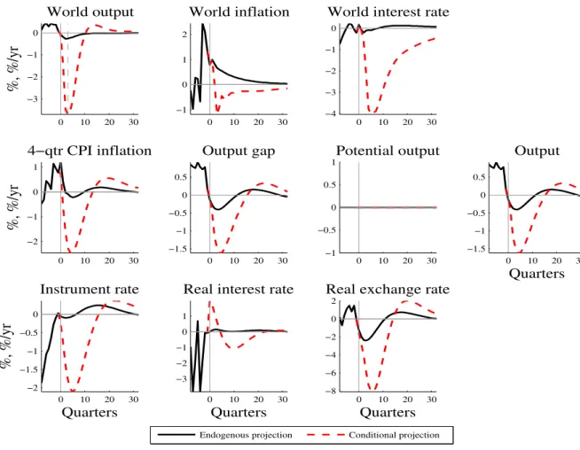
Figure 5.1 show projections from Ramses using data up to and including 2008:2, for 10 key variables: foreign output, foreign annualized 1-quarter CPI inflation, foreign interest rate, the real exchange rate, 4-quarter CPI inflation, the output gap, the instrument rate, the real interest rate (the instrument rate less 1-quarter-ahead CPI inflation expectations), output and potential output. The plots show deviations from steady state. The solid vertical line marks2008:3, which is quarter 0 in thefigure. The curves to the left of the line shows the history of actual data up to and including

2008:2, which is quarter -1 in the figure. The state in 2008:2, and its history, is estimated using policy with the instrument rule.

The solid curves to the right of the solid vertical line show the projections for a policy maker following the estimated instrument rule. We see that Ramses’ VAR-model for the three foreign variables did not forecast the large drop in the world economy that occurred in the next few quarters after 2008:3, following the turbulence in the financial markets. In reality, world output diminished by almost4percent in the next three quarters and world inflation approached0percent. Given the VAR-model’s counterfactual view of the foreign economy, Ramses projected Swedish CPI inflation to be close to 2 percent and output to be less than05 percent below its trend level. Ex post, we know Swedish GDP decreased by almost 6 percent in the next year and consumer prices actually declined.

We know from VAR evidence that international spillover effects to small open economies are generally large. Lindé [18] shows, using a block exogenity assumption in a VAR model on Swedish

2 2