2008/14
■
Compatibility choice
in vertically differentiated technologies
CORE
Voie du Roman Pays 34
B-1348 Louvain-la-Neuve, Belgium. Tel (32 10) 47 43 04
Fax (32 10) 47 43 01
E-mail: [email protected] http://www.uclouvain.be/en-44508.html
CORE DISCUSSION PAPER 2008/14
Compatibility choice in vertically differentiated technologies Filomena GARCIA 1 and Cecilia VERGARI2
March 2008 Abstract
We analyse firms' incentives to provide two-way compatibility between two network goods with different intrinsic qualities. We study how the relative importance of vertical differentiation with respect to the network effect influences the price competition as well as the compatibility choice. The final degree of compatibility allows firms to manipulate the overall differentiation. Under weak network effect, full compatibility may arise: the low quality firm has higher incentives to offer it in order to prevent the rival from dominating the market. Under strong network effect we observe multiple equilibria for consumers' demands. However, in any equilibrium of the full game, coordination takes place on the high quality good which, we assume, always maintains its overall quality dominance.
Compatibility is always underprovided from the social point of view. Keywords: compatibility, vertical differentiation, network effect. JEL Classification: L13, L15
1 ISEG, TULisbon, Technical University of Lisbon and UECE, Lisbon, Portugal. E-mail:
2CORE, Université catholique de Louvain, Belgium; University of Roma TRE and University of Bologna,
Italy. E-mail: [email protected]
We are grateful to Oscar Amerighi, Rabah Amir, Emanuele Bacchiega, Paul Belleflamme, Giuseppe De Feo, Vincenzo Denicolo, Mario Denni, Jean Gabszewicz, Luca Lambertini, Mario Tirelli, Vincent Vannetelbosch, Xavier Wauthy, and seminar audiences at FUSL, CREI and ISEG for useful comments and discussion about an earlier draft.
This paper presents research results of the Belgian Program on Interuniversity Poles of Attraction initiated by the Belgian State, Prime Minister's Office, Science Policy Programming. The scientific responsibility is assumed by the authors.
1
Introduction
On March 2003, Sony announces that it is ready to deliver its first blue-laser DVD recorder (Blu-Ray), which will allow discs to hold up to five times more data than current DVD models. HD-DVD format constitutes its main rival, although the storage potential is around 40 percent lower for HD-DVD disks, its technology is less expensive and can be available sooner. In the war for standards, timing can be crucial, as consumers regard the installed network, before making a decision. Both HD-DVD and Blu-Ray developers have taken this into account, by allowing their players to be compatible with existing DVD technology (backward compatibility). However, both work separately without considering (to the present), the possibility of rendering their players compatible with the rivals disc format. The purpose of this paper is to analyse the incentives to render compatible two standards with different intrinsic qualities, which compete in prices in the product market. Another example of network goods with different intrinsic qualities is MAC vs Microsoft Windows operating systems, where it is widely recognized that Microsoft has captured the largest market share with lower prices, whereas Apple Macintosh has proved to be a higher quality product (for instance in terms of high resolution graphics).
Compatibility represents an important issue in network industries. Indeed, firms de-cide whether to make their goods compatible with those of their rivals, thus competing in the market, or to make them incompatible thus competing for the market (standard war). As Besen and Farrell (1994) put forward, “there is no general answer to the ques-tion of whether firms will prefer competiques-tion for the potentially enormous prizes under inter-technology competition, or the more conventional competition that occurs when there are common standards. Indeed, the same firms may choose different strategies in different situations”. A recent example (October 2005), is Microsoft and Sony Team on Digital Entertainment Content Management System: though rivals in the gaming-console market, both companies find they have much to gain from working closely to integrate the new Sony VAIO XL1 Digital Living System with Microsoft Windows XP Media Center Edition 2005.1
Mainly, there are two ways to ensure compatibility: standardization, that is firms may bring products to a uniform standard and theprovision of a converter, that is firms may produce a device which allows consumers from one side of the market to enjoy some compatibility with the network of the other side. A converter can be either one-way
or two-way depending on whether the benefits for the consumers are private or public.
In the case of one-way converter, consumers from each side of the market enjoy the opposing network in an unilateral fashion. For instance, if a device is created to allow HD-DVD discs to be read by Blu-Ray players (even though quality might be imperfect), this would allow the owners of Blu-Ray players to enjoy not only the Blu-Ray network but also the HD-DVD network (at least partially). Nevertheless, HD-DVD player owners could not use the same device likewise. Consequently, the benefits stemming from a one-way converter are private. Also, when firms decide to offer a one-one-way converter, they
choose the degree of compatibility separately from each other.
In the case of two-way converter, consumers from each side of the market enjoy the opposing network in a bilateral fashion. This would correspond to the existence of a de-vice that allows both Blu-Ray and HD-DVD players to read the discs of the opponent’s format (even though conversion might also be imperfect). The benefits stemming from a two-way converter are then public. Depending on the specificities of the technologies involved, we can have two situations. First, both firms may have to contribute to the quality of compatibility, and as such, contributions are complementary. This situation has been modeled by Cr´emer et al. (2000) while discussing the interconnectivity be-tween internet backbones. The idea is that the quality of the interconnection is the minimal of the qualities offered by each backbone. This is sensible as their problem entails communication networks and it is clear that both parties must contribute for good communication. Second, each firm may be able to successfully provide a two-way converter, not being necessary that both contribute to the quality of the device. In this case contributions are substitutes. We can find examples in the network formation lit-erature: Bala and Goyal (2000) refer to the phone call where only the caller has to pay, however information can be exchanged by both parties. Also, Bloch and Dutta (2005) model separable investment implying non complementarity in the link formation. Re-calling the Blu-Ray vs HD-DVD example, we can think of both producers having the incentive to provide a two-way converter, but finally agreeing on using the most efficient one i.e. the level of compatibility will be the maximal between the levels chosen by each firm. The complementarity or substitutability among converters can also depend on the status of firms’ property rights. Indeed, it can be the case that a firm needs a license to develop a converter and to make its good compatible with a rival good.
In the present article we investigate the provision of substitutable two-way converters in a setup where firms are vertically differentiated. We also compare the private and social incentives towards compatibility. To this end, we develop a two-stage game where firms first choose the degree of compatibility and then the price of their products. Finally, consumers buy one unit of either good.
The main finding is that the interaction between the intrinsic quality differentiation and the importance of the network effect leads to different market configurations which in turn imply different incentives to provide compatibility. This is due to the fact that the degree of conversion, hence the final network size, affects the overall product differentiation. Under weak network effect, i.e., when the weight of the network effect relative to the vertical differentiation is not very strong, we can observe full compatibility at equilibrium. In this case, where both firms may remain active in the market, they are willing to offer it because an increase in the conversion level makes competition milder. However, the low quality firm has higher incentives to provide full compatibility in order to avoid the possibility of being stranded out of the market. On the other hand, under strong network effect, i.e., when the network effect dominates the vertical differentiation, we observe multiple equilibria for consumers’ demands. Namely, as consumers value very highly the network, they can all coordinate on either the high quality or the low quality good. However, in any equilibrium of the full game, coordination takes place on the high quality good which, we assume, always maintains its overall quality dominance.
To sum up, we show that both firms may have incentives to provide compatibility. In spite of that, as long as the network effect is not high enough to allow a switch in the overall quality differential, the low quality firm is willing to pay more for compatibility. Concerning the social incentives, we find that compatibility is always underprovided.
In the theoretical literature, we can distinguish between compatibility strategies towards horizontal and vertical competitors. As far as the first strand is concerned, to which this work is directly linked, Cremer et al. (2000) who consider an extension of the seminal paper by Katz and Shapiro (1985), study compatibility decisions in a Cournot oligopoly with homogeneous goods and heterogeneous consumers, where firms differ in their installed base of consumers. The standard result predicts that smaller firms always have higher incentives for product compatibility than bigger firms. To our knowledge, only Baake and Boom (2001) study firm’s compatibility decisions in a framework of vertical differentiation. As Cremer et al. (2000), they model compatibility as a firms’ complementary decision; however, it is a zero-one choice. In line with this literature, they show that the high quality firm, in contrast with the rival firm, is against compatibility.
As for the second strand, there is a literature that is related to firms’ compatiility strategy towards vertically related firms, the suppliers of complementary goods. Theo-retical models distinguish according to whether each component is sold by an indepen-dent firm or each firm produces everything necessary to form the final good (system).2 Farrell et al. (1998) make the distinction between competing on final products only (closed organization), or competing at intermediate stages components as well as on final products (open organization). As they state, “in the 1980s, the industry gener-ally evolved towards an open structure, in which hardware systems are composed of independently produced components combined through standardized interfaces with, in general, several competing providers of each component [...] More recently, however, the software side has arguably become increasingly closed as more and more functionality is built into the Microsoft operating system and user interface.”
The structure of the paper is as follows. Section 2 describes the model, Section 3 provides the main results on the price competition and compatibility choice by firms and, finally, Section 4 presents the socially optimal compatibility level and compares it with the private incentives.
2
Model
Two firms, A and B, produce competing technologies at constant marginal cost set to zero. These technologies are vertically differentiated and characterized by network externalities in consumption, i.e. consumer’s utility is increasing in the number of con-sumers that choose the same technology. Firms may decide to render the technologies
2As an example of the first context, Church and Gandal (1992) study the software provision decision
of software firms to hardware firms. As for the case of firms supplying all the necessary components, Matutes and Regibeau (1992), which extend Matutes and Regibeau (1988), study firms’ incentives to standardize components in industries where consumers try to assemble a number of components into a system that meets their specific needs.
compatible through a converter whose quality determines the degree of network ben-efits that the consumers enjoy from the rival technology. Hence, consumers’ utility is a function of the intrinsic quality of the technology, of the size of the network and of the compatibility that can be achieved with the rival network. We assume that there is a continuum of consumers indexed by x which is uniformly distributed in the inter-val [0,1]. Thus, x measures consumers’ valuation of the quality: high consumer types value quality improvements more than low consumer types.3 Each consumer has a unit
demand and buys either one unit of good A or one unit of good B. We rule out the possibility of no purchase, that is we concentrate on the situation in which the market is fully covered.4
We assume that consumer’s utility takes the following standard form: UA(x) =βAx+α[DA+τ DB]
UB(x) =βBx+α[DB+τ DA]
The first term of the utility function, βix is the stand alone value of the technology
for consumer type x. The parameter βi represents the quality of technology i and we
assume throughout that βB > βA, i.e., the intrinsic quality of technology B is higher
than that of technologyA. The second term in the utility is the network benefit, where the parameter α >0 denotes the intensity of the network effect and Di is the demand
of technology i. Therefore, consumers differ in their valuation of the intrinsic quality but value equally the network effect. The latter consists of the externality coming from the interaction with consumers that buy the same technology, (Di), and the externality
resulting from the existence of a converter, which allows consumers to partially benefit from the rival network (τ Dj).
The final quality of conversion is endogenous and given by τ ∈ [0,1] which is a function of the degrees of conversion chosen by each firm, τA and τB, respectively. In
order to model a two-way converter, we assume that τ = max{τA, τB}. Underlying
this formulation is the idea that the devices produced noncooperatively by each firm are substitutes in the sense that the compatibility achieved by the consumers of one technology is also achieved by the rival consumers. As such, the final compatibility is the maximum of the levels chosen by the firms. There is a linear cost of producing the converter which is increasing in τi and given by cτi. We assume that firms are equally
efficient in producing the converter and thus face the same cost function.
The final level of conversion influences the overall quality differential between the technologies, which is then determined by two sources of quality differentiation. The first one is exogenous and given by k≡βB−βA and the other, endogenous, is proportional
to the difference in the networks’ size and given byα(DB−DA)(1−τ). The endogenous
source of differentiation can be manipulated by the firms through the choice of prices and
3We discuss about alternative asymmetric distributions for consumer types in Appendix 6.1. The
intuitive result is that the more consumers are concentrated around zero (one), the more firmA(B) has a demand advantage.
4We also exclude the possibility for consumers to join both networks. This could be an alternative
through the choice of the conversion level (τ). We define the overall quality differential as:
k+α(DB−DA)(1−τ).
We can interpret this expression as follows: when either the two networks have the same size (DA=DB) or compatibility is perfect (τ = 1), consumers perceive the technologies
as being identical in terms of the network effect.
We assume throughout the paper that the overall quality of goodB is higher than that of good A. A sufficient condition for this is k≥a(1−τ), i.e. even in the extreme case that the network benefit for firm A is the highest (DA= 1 and DB = 0), good B
maintains its quality dominance.
Both firms decide first the quality of the conversion that they are willing to offer their consumers and then compete in prices. We model their decisions as a two stage game and as such the solution concept that we will be using is the subgame perfect Nash equilibrium.
Consumers choose between the technologies maximising their net surplus. In this maximization problem they take as given the decisions of the other consumers. We assume that consumers have rational expectations about the size of the networks. Con-sumerxbuys technologyAif and only ifUA(x)−pA> UB(x)−pBandUA(x)−pA>0.
Denote ˆx the consumer type which is indifferent between the two technologies and as-sume that the typex= 0 has positive net utility from buying productA, i.e. UA(0)−pA
is nonnegative.5 Demands are then given by DB = 1−x,ˆ
DA= ˆx.
We analyse the situation where both firms face a nonnegative demand, ˆx∈[0,1]. There are three possible market configurations:
1. DA = 1 and DB = 0. In this case, the utility of consumers becomes UA =
βAx+α −pA and UB = βBx+ατ −pB. For this market configuration to be
possible, all consumers, even consumer type x = 1 should prefer to buy good A, i.e. pB−pA≥k−α(1−τ).
2. DA = 0 and DB = 1. In this case, the utility of consumers becomes UA =
βAx+ατ −pA and UB = βBx+α−pB. For this market configuration to be
possible, all consumers, even consumer type x= 0 should be interested in buying goodB, i.e. pB−pA≤α(1−τ).
3. DA, DB ∈ (0,1) and DA+DB = 1. In this market configuration both firms set
positive prices and obtain positive profits.
5The market coverage assumption in this model wherex∈[0,1] is only possible thanks to the presence
of positive network effects. Indeed, with α >0, consumer type zero may prefer buying because even if its valuation of the intrinsic quality is zero he benefits from the network of consumers buying the same good or compatible goods.
The market configurations described above occur when the following conditions on the variables of the model hold:
pA−pB ≤α(1−τ) (DA−DB), (1)
pB−pA≤α(1−τ)(DB−DA) +k, (2)
pA≤α(DA+τ DB). (3)
Condition (1) corresponds toUA(0)−pA≥UB(0)−pB. In words, consumer typex= 0
prefers good A: the price difference between product A and B must be compensated by the gain in terms of the network effect, since he has no valuation for the intrinsic benefit of the good. In particular, we can interpret the RHS of condition (1) in the following way: if no conversion is available,τ = 0, then what it takes to compensate for the difference in prices is α(DA−DB). Since there is a converter, the compensation can
be smaller (as τ <1).
Condition (2) corresponds toUA(1)−pA≤UB(1)−pB. In words, consumer typex=
1 prefers good B. The price difference between productB andA must be compensated by the advantage of buying B i.e., by the difference in the network effect and the difference in the intrinsic qualities (since the consumer located atx= 1 cares about the intrinsic benefit as well as the network benefit).
Condition (3) corresponds toUA(0)−pA≥0. In words, consumer typex= 0 prefers
buying good Ato not buying anything if and only if the benefit which he obtains from the network exceeds the price.
The indifferent consumer is: ˆ
x=α(1−τ)DA−DB
k +
pB−pA
k , (4)
which implies that demands, in the interior solution case, are given by: DA= k−−α2α(1(1−−τ)τ)+k−p2Bα−(1p−Aτ),
DB = kk−−2αα(1(1−−ττ)) −k−p2Bα−(1p−Aτ).
Observing these expressions, we see that depending on the sign of k−2α(1−τ) they are either decreasing or increasing in own price. In what follows we distinguish the two cases.
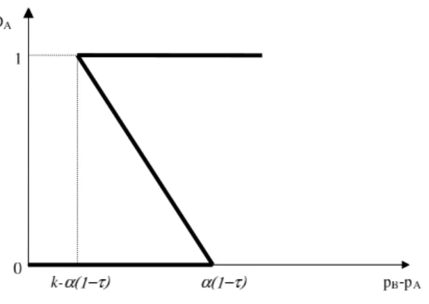
• Weak Network effect. Assume first thatk >2α(1−τ), such thatDAand DB are
decreasing in own price.
DB= 1, pB−pA≤α(1−τ) k−α(1−τ) k−2α(1−τ)− pB−pA k−2α(1−τ), α(1−τ)< pB−pA≤k−α(1−τ) 0, pB−pA> k−α(1−τ) (5) DA= 1, pB−pA> k−α(1−τ) −α(1−τ) k−2α(1−τ)+ pB−pA k−2α(1−τ), α(1−τ)< pB−pA≤k−α(1−τ) 0, pB−pA≤α(1−τ) (6)
Figure 1: Demand functions: k >2α(1−τ).
Figure 2: Demand for network goodA: k <2α(1−τ).
• Strong Network effect. Assume now thatk <2α(1−τ). The network effect plays a dominant role in the differentiation among products. As such, multiple equilibria in the consumers’ game arise. In particular, as illustrated in Figure 2 for good A, the demands for the network goods are correspondences:
DB= 1, pB−pA≤α(1−τ) −k+α(1−τ) 2α(1−τ)−k + pB−pA 2α(1−τ)−k, k−α(1−τ)≤pB−pA≤α(1−τ) 0, pB−pA≥k−α(1−τ) (7) DA= 1, pB−pA≥k−α(1−τ) α(1−τ) 2α(1−τ)−k− pB−pA 2α(1−τ)−k, k−α(1−τ)≤pB−pA≤α(1−τ) 0, pB−pA≤α(1−τ) (8)
For the range of prices such thatpB−pA∈[k−α(1−τ), α(1−τ)] there are three
possible equilibria: either they all coordinate on good A or they all coordinate on good B or some consumers prefer good A and others prefer good B. Notice
that in the last case, demands are increasing in own price. This is due to the fact that when deciding between A and B consumers value mostly the dimension of the network that they will enjoy. Thus, as demands increase, also the value of the goods does and in turn the consumer’s willingness to pay increases.
In all cases, consumers’ expectations are rational and none of these equilibria is Pareto dominant. Therefore, we cannot select any of them.
A complete analysis of the feasible price regions determined by the conditions (1)-(3) and consumers’ demands can be found in Appendix (6.2).
3
The characterization of equilibria
3.1 Price competition under weak network effect
In the second stage of the game, firm ichooses its price pi so as to maximize its profit
Πi:6
Πi(pi, pj) =piDi(pi, pj), withi6=j andi, j=A, B
Under weak network effects, i.e. whenk >2α(1−τ), the demands for the network goods are well defined functions, in particular they are linear and decreasing in own price. We can therefore proceed by computing firms’ reaction functions. Given demands (5) and (6), the profits are:
ΠB = pB, pB−pA≤α(1−τ) k−α (1−τ) k−2α(1−τ)+ pA−pB k−2α(1−τ) pB, α(1−τ)< pB−pA≤k−α(1−τ) 0, pB−pA> k−α(1−τ) ΠA= pA, pB−pA> k−α(1−τ) −α(1−τ) k−2α(1−τ)+ pB−pA k−2α(1−τ) pA, α(1−τ)< pB−pA≤k−α(1−τ) 0, pB−pA≤α(1−τ)
The following Lemma characterizes the reaction functions on prices of firms under the weak network effect assumption.
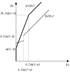
Lemma 1 Fork >3α(1−τ), the reaction function of firmB is given by,
pB(pA) = 1 2(k−α(1−τ)) + pA 2 , if pA≤k−3α(1−τ) α(1−τ) +pA, if pA> k−3α(1−τ)
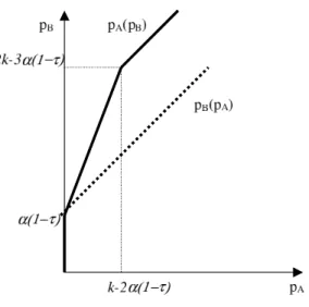
Whereas for 2α(1−τ)< k≤3α(1−τ), the reaction function is:
pB(pA) =pA+α(1−τ)
6We here forgo the compatibility costs to simplify the presentation but this is without loss of
Figure 3: Reaction functions: k >3α(1−τ).
As for firm A, the reaction function, for k >2α(1−τ), is
pA(pB) = pA= 0, pB≤α(1−τ) pB−α(1−τ) 2 , ifα(1−τ)< pB≤2k−3α(1−τ) pB−k+α(1−τ), if pB >2k−3α(1−τ)
Proof. See Appendix (6.3.1). The reaction curves are depicted in Figure 3 for the case k >3α(1−τ), and in Figure 4 for the case 2α(1−τ)< k≤3α(1−τ). From the observation of the reaction functions, it is easy to see that:
1. When k >3α(1−τ), there exists a unique Nash equilibrium of the price game, given by7
p∗A= 1
3k−α(1−τ), (9)
p∗B= 2
3k−α(1−τ). (10)
The corresponding equilibrium demands are DA∗ = 1 3 k−3α(1−τ) k−2α(1−τ), (11) D∗B= 1 3 2k−3α(1−τ) k−2α(1−τ) . (12)
7By solving the system, it is easy to see that the computed price equilibrium is the unique intersection
Figure 4: Reaction functions: 2α(1−τ)< k≤3α(1−τ).
Notice that in this price equilibrium, a necessary condition for the market coverage assumption to hold is k ≤3.46α.8 When the vertical differentiation is very high (k >3.46α), consumer type zero prefers not buying rather buying good A whose quality is relatively very low.
2. When k∈ (2α(1−τ),3α(1−τ)], there exists a unique Nash equilibrium of the price game, given by
p∗A= 0,
p∗B=α(1−τ), where D∗
A= 0 and DB∗ = 1.
As in the classical model of vertical product differentiation the firm that produces the high quality good charges a higher price. For high intrinsic quality differences, k > 3α(1−τ), prices are increasing in the degree of conversion and in the intrinsic vertical differentiation,k. When consumers value highly the network, or in other words, when α is large, firms behave more competitively in order to gain network advantage. This implies that prices are decreasing in α.This effect becomes milder in the presence of a converter. Compatibility renders the network size less important for consumers and therefore prices increase with τ.
On the contrary, when the intrinsic quality difference is lower,k∈(2α(1−τ),3α(1−τ)], the high quality firm is the only active firm in the market. In that case a higher valu-ation of the network allows the firm to extract a higher consumer surplus by setting a
8Formally, U
A(0)−pA ≥ 0 ⇐⇒ k2−3α(2−τ)k+ 3α2(1−τ)(3−τ) < 0 whose solution is
k∈[k1(τ), k2(τ)]; where k1(τ) is a decreasing and convex function andk2 is a concave function whose
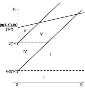
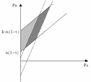
Figure 5: Price space forα(1−τ)< k <2α(1−τ).
higher price. Also, as τ increases, the overall quality differential becomes lower and as such price competition intensifies. In order to maintain the whole market, firmB needs to set a lower price.
3.2 Price competition under strong network effect
For the strong network effect case, α(1−τ) < k <2α(1−τ), we need to consider the demands (7) and (8). Then, profits are given by
πB = 0, pB−pA≥k−α(1−τ) α(1−τ)−k 2α(1−τ)−k + pB−pA 2α(1−τ)−k pB, k−α(1−τ)≤pB−pA≤α(1−τ) pB, pB−pA≤α(1−τ) πA= 0, pB−pA≤α(1−τ) α(1−τ) 2α(1−τ)−k − pB−pA 2α(1−τ)−k pA, k−α(1−τ)≤pB−pA≤α(1−τ) pA, pB−pA≥k−α(1−τ)
Profits are nondecreasing in own price, hence firms have incentive to set prices as high as possible. Given the market coverage assumption, prices are bounded from above. Moreover, the existence of multiple consumer partition equilibria suggests for multiple price equilibria. In order to solve the price competition stage, consider the relevant price region depicted in Figure 5. We divide this price space in 5 regions that we analyse in turn.
In regions I and II, there is a unique consumer partition equilibrium: (D∗
A= 0, DB∗ =
1) and (D∗
A= 1, D∗B= 0), respectively. In these regions, no price equilibrium exists: in
In regions IV and V, all three consumer partitionsDA= 1,DA= 0 andDA∈(0,1)
are equilibria of the consumers’ choice. We proceed by first eliminating the consumer partitions which are not compatible with a price equilibrium in these regions. Concerning region IV,DA= 1 can never be part of the equilibrium of the full game because firmB
can always reduce its pricepB and conquer a positive market share (going to region I).
In contrast, for DB = 1, given anypB belonging to region IV, firmAcannot profitably
deviate as its profit is zero in any case. Therefore, in region IV any price pair (pA, pB)
such that pA≥0 and pB is α(1−τ) is an equilibrium . Concerning region V, no price
equilibrium can be associated with either DA = 1 or DB = 1 because the firm with
no consumers can always reduce its price and obtain positive profit, (pA can decrease
and reach region II and similarly pB can decrease and reach region I). We conclude by
considering the possibility of DA∈(0,1) in regions IV and V.
Lemma 2 Let k < 2α(1−τ), the reaction functions of firms A and B in regions IV
and V with DA∈(0,1), are given by,
pB(pA) = ( α(1−τ) +pA, if pA≤ατ α(1−τ2)−kτ 1−τ +pA (k−α(1−τ)) α(1−τ) , if pA> ατ pA(pB) = pB−k+α(1−τ), if pB≥k−α(1−τ) 0, if pB< k−α(1−τ)
Proof. See Appendix 6.3.2. Drawing these reaction functions, we can easily see that they intersect only once at pA = α and pB = k+ατ. However, such a price pair is
incompatible with the consumer partitionDA∈(0,1). Indeed, as Figure 2 illustrates, at
pB−pA=k−α(1−τ), the equilibrium consumers’ choice is eitherDA= 0 orDA= 1.
Finally, in region III, we have a unique equilibrium of the consumers’ choice: any price pair (pA, pB) such thatpB ≤k−α(1−τ) and pA≥0 is associated with DA= 0,
DB= 1. Profits are then ΠA= 0 for firm Aand ΠB =pB for firmB: thus, firmA will
be indifferent between any pA≥0; however, firmB would always have an incentive to
increase pB so as to move to region IV (as long as pA is sufficiently low), where it can
set a higher price.
Summing up, forα(1−τ)≤k <2α(1−τ), there exist multiple equilibria for the price subgame. Namely, any price pair (pA, pB) such thatpB =α(1−τ) andpA≤2α(1−τ)−k
associated withDB= 1 is an equilibrium. In order to solve the compatibility stage, and
in turn the full game, in what follows we select the particular price equilibrium such that pA= 0 and pB=α(1−τ) withDA= 0 and DB = 1.
In the strong network effect case, consumers exhibit what is known as strong
con-formity (Grilo et al. 2001). This means that consumers would like to coordinate their
choices on the same good in order to enjoy the maximum network effect because the difference in intrinsic qualities is not relevant. However, as the overall quality of good B is still superior, at equilibrium, coordination takes place on the high quality good B. Notice that if we letk < α(1−τ), a switch in the overall quality occurs and coordination could also take place on good A.
3.3 Compatibility choice
Let us now analyse the first stage of the game. Consider that the firms choose their compatibility levels noncooperatively and assume that the global conversion is given by τ = max{τA, τB}. As seen in the price competition, there are different price
equi-libria depending on the relative weight of the intrinsic quality and the network effect. Accordingly, we have the three following cases for the overall profits of firms.
Case 1 Interior solution in prices k >3α(1−τ) ⇐⇒ τ ∈(3α−k
3α ,1] ΠIA= (α(τA−1)+13k)2 k−2α(1−τA) −cτA ifτA≥τB (α(τB−1)+13k) 2 k−2α(1−τB) −cτA ifτA< τB (13) ΠIB = (α(τA−1)+23k) 2 k−2α(1−τA) −cτB ifτA≥τB (α(τB−1)+23k)2 k−2α(1−τB) −cτB ifτA< τB (14)
Case 2 Corner solution in prices k∈[2α(1−τ),3α(1−τ)] ⇐⇒ τ ∈[2α2−αk,3α3−αk]
ΠCA = 0−cτA (15)
ΠCB =
α(1−τA)−cτB ifτA≥τB
α(1−τB)−cτB ifτA< τB (16) Case 3 Strong network effect case where k ∈ [α(1−τ),2α(1−τ)) or τ ∈ [0,2α−k
2α ).
In order to illustrate such a possibility characterized by multiple price equilibria, we pick the one where pA = 0 and pB = α(1−τ) and consumers coordinate on
goodB which implies
ΠSA= 0−cτA,ΠSB=
α(1−τA)−cτB ifτA≥τB
α(1−τB)−cτB ifτA< τB
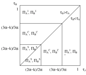
To analyse the compatibility game we must consider three regions for the parameters (as Figure 6 illustrates):
i) 3α−k
3α ≤0,in which case for all values of τA and τB, the unique outcome of the price
competition stage is the interior solution.
ii) 2α2−αk <0< 3α3−αk, in which case, for values ofτA, τB∈[0,3α3−αk), we have the corner
solution in the price competition stage and for values ofτA, τB ∈(3α3−αk,1] we have
the interior solution in the price competition stage.
iii) 0 ≤ 2α2−αk < 3α3α−k, in this case, we have that for values of τA, τB ∈ [0,2α2−αk) the
outcome of the price competition stage is the one assumed in the strong network effect case (considering a particular price equilibrium is the only way to solve the compatibility game for this range of parameters); for τA, τB ∈[2α2−αk,3α3−αk), the
outcome of the price competition stage is the corner solution and for τA, τB ∈
[3α−k
Figure 6: Parameters space for the compatibility
Notice however that the corner solution and the strong network effect solution of the price competition stage coincide, i.e., ΠC
A = ΠSA and ΠCB = ΠSB, therefore the last two
regions can collapse in one.
The following Proposition presents the results for the compatibility game for each partition of the parameter space defined above.
Proposition 3 When the intrinsic quality differentiation is very high with respect to
the network effect (k >3α) firms have the incentive to choose full compatibility, as long
as the cost is not too high. However, when the result is either full or no compatibility, low consumer types prefer not to buy anything.
In contrast, when the intrinsic quality differentiation, k, is low, but still the high
quality good maintains its quality dominance, (α < k ≤ 3α), the outcome of the
com-patibility game is compatible with market coverage. It yields full comcom-patibility (τ = 1)if
and only if the cost is low, namely, c < k9. For higher conversion costs, the equilibrium
compatibility between the two network goods is zero. Proof. See Appendix (6.3.3).
This proposition highlights the incentives of the firms to provide two way compat-ibility depending on the relative importance of the network effect versus the intrinsic quality. The following table summarizes our results.
α−k α <0≤ 3α−k 3α c= 0 τA= 1, τB ∈[0,1] τB= 1, τA∈ 9α−4k 9α ,1 τ = 1 0< c < (4k−99α) τA= 1, τB = 0 τB= 1, τA= 0 τ = 1 (4k−9α) 9 < c < k9 τA= 1, τB = 0}τ = 1 c > k9 τA= 0, τB = 0}τ = 0
Proposition 3 deserves a closer analysis. Concerning the first statement, we find that in a market where the products have a very high intrinsic quality differentiation with respect to the network effect (k > 3α) firms have the incentive to choose full compatibility for low cost levels. Indeed as the degree of compatibility increases, the price competition softens. However, when the result is either full or no compatibility, low consumer types prefer not to buy anything. Namely, when compatibility is absent the quality of goodA is so low with respect to the quality of goodB that low consumer types do not buy it. On the other hand, when compatibility is full, although the overall differentiation decreases, the price increase prevents some consumers from buying.
As for the second statement, we also find that firms have incentive to provide full compatibility for small levels of its cost. However, the lower intrinsic quality differenti-ation allows for a market coverage equilibrium. Looking at the particular behavior of each firm, we can see from the table that as long as 0< c < (4k−99α), the game has two Nash equilibria: (τA = 1, τB = 0) and (τA = 0, τB = 1). This is due to the fact that
reaction functions are discontinuous and have a unique downward jump. Intuitively, when the opponent chooses a level of conversion high enough, not necessarily 1, the firm prefers to enjoy this level of conversion rather than paying for the converter. Further-more, when (4k−99α) < c < k9, in equilibrium, only the low quality firm has incentive to offer compatibility. This is so, because, otherwise, firm B would be in a position to dominate completely the market. By offering compatibility, firm A attracts consumers and becomes active in the market.
From the table, we can also notice that wheneverc >0, firms never incur in wasteful duplication of compatibility costs. Indeed, at any equilibrium, there is only one firm providing a converter device.
In the following, we present the equilibrium results for all the relevant variables. When the vertical differentiation is such that α < k≤3α, equilibrium prices demands and profits depend on the compatibility cost in the following way. If c < k9, which implies τ = 1 and in turn the interior solution in prices,
DA∗ = 1 3,D ∗ B= 2 3 p∗ A= k 3,p ∗ B = 2k 3 . Profits are then either, Π∗
A= k9 −cand ΠB∗ = 49k or Π∗A= k9 and Π∗B = 49k−c. Ifc≥ k9,
which implies τ = 0 and in turn the corner (or the strong network effect) solution in prices,
D∗A= 0, DB∗ = 1 p∗A= 0, p∗B =α
4
Welfare
We next investigate whether the equilibrium compatibility level is optimal from a social welfare point of view. That is, we let the social planner choose the compatibility level, τ at a cost cτ and firms compete in prices, as before. This implies that now firms’ profits do not include the compatibility cost, as it is incurred only by the social planner.
Define, as usual, the social welfare by the following expression: SW = Z bx 0 (UA(x)−pA)dx+ Z 1 b x (UB(x)−pB)dx+ ΠA+ ΠB−cτ. (17)
As before we need to distinguish the possible equilibria of the price competition stage.
• When k >3α(1−τ) ⇐⇒ τ ∈(3α3−αk,1], SWI =βB 1 2 − τ3−k218α(4−3τ) + 9kα2(1−τ) (17−9τ) 18 (k−2α+ 2ατ)2 −cτ. • When k∈[α(1−τ),3α(1−τ)] ⇐⇒ τ ∈[α−αk,3α3−αk], SWC = 1 2βB+ατ+α(1−τ)−cτ = 1 2βB+α−cτ.
The following proposition summarizes the results for the optimal compatibility choice of the social planner.
Proposition 4 For very high intrinsic quality differentiation, (k >3α) the social wel-fare is maximized by full compatibility, however, this outcome is not consistent with the assumption that the market is covered. In contrast, when the intrinsic quality
differenti-ation is not too high with respect to the network effect (α < k≤3α), market coverage is
the equilibrium outcome: full compatibility is the optimal solution from the social point of view when the cost is low. When cost is intermediate, the social planner chooses
partial compatibility τ = 3α3−αk. Finally for high costs, no compatibility is the preferred
solution.
Proof. See Appendix 6.3.4
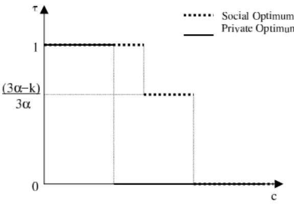
We can now discuss how the welfare maximising solution differs from the private optimum. We always observe underprovision of compatibility. Firms are willing to offer full compatibility for a smaller range of the costs than the social planner. This result is rather intuitive. Compatibility in our context is a public good as both firms attain the same level of compatibility even if the investment is provided unilaterally. Figure 7 illustrates the private and social choice of compatibility for different levels of cost.
Figure 7: Private versus Social Choice,α < k <3α.
5
Conclusion
In this paper, we have analysed firms’ incentives to provide two-way compatibility be-tween two network goods with different intrinsic qualities, assuming substitutability between the converters. Our results show that firms may be willing to offer some pos-itive compatibility also on their own, that is not being necessary that both contribute to the quality of the device.
Assuming that the good with higher intrinsic quality always maintains its overall quality dominance, we have provided a complete analysis by studying how the relative importance of vertical differentiation with respect to the network effect influences the price competition as well as the compatibility choice. Indeed, the final degree of com-patibility allows firms to manipulate the overall product differentiation. Namely, when consumers’ valuation of the network is not high enough to allow an overall quality switch of the vertically differentiated goods, full compatibility may arise: the low quality firm has higher incentives to offer it in order to prevent the rival from dominating the mar-ket. Comparing firms’ compatibility decisions with the social optimum, we show that compatibility is always underprovided. This result comes from the nature of a two-way converter which actually is a public good.
Our analysis points out new interesting results about firms’ incentives to offer two-way compatibility. Indeed, as Besen and Farrell (1994) describe, firms’ horizontal com-patibility strategies determine the form of competition in the market. In particular, with two firms, there are three combinations of such strategies: both firms choose incompat-ibility which results in a standard war; both firms prefer compatincompat-ibility; and finally, one firm chooses incompatibility whereas the other prefers compatibility. The last is the only case where firms choose different strategies. This seems reasonable when firms are asymmetric. For example, Katz and Shapiro (1985) show how a larger firm is more likely to prefer incompatibility than a smaller firm. However, we show that this need not be the case. In fact, for high levels of quality differential both firms have incentives to provide compatibility while for low levels of quality differential they may have
asym-metric preferences. When vertical differentiation is very high, competition is mild and both firms manage to stay in the market: offering compatibility they can further soften competition because consumers’ valuation of the goods increases. In contrast, for low levels of vertical differentiation, either the high quality firm or the low quality firm are likely to conquer the market thus having opposite incentives for compatibility.
In our future agenda, we propose to extend the model by considering the possibility of a switch in the overall quality differential, i.e., the case where the overall quality of the high quality good is lower than that of the low quality good thanks to the magnitude of the network effect. Preliminary results suggest that the firm with lower intrinsic quality could conquer the market thus being the high quality firm who has more to gain from compatibility.9
We are also interested in investigating firms’ strategic incentives to provide one-way compatibility towards horizontal competitors in the context of vertical differentiation.10
In this case, the benefits stemming from the converter are private. The analysis should thus reverse. Again, according to the relative weight of vertical differentiation, compat-ibility would affect the degree of competition between network goods’ suppliers in the opposite way.
6
Appendix
6.1 Consumer types distribution
Throughout the model, we assume that consumers indexed by x are uniformly dis-tributed in the interval [0,1]. The uniform distribution can be seen as a particularBeta distribution with parametersaandbsuch thata=b= 1. Formally, the Beta cumulative distribution function is F(x;a, b) = Γ(a+b) Γ(a)Γ(b) Z x 0 ua−1(1−u)b−1du,
with a > 0, b > 0 and x ∈ [0,1]. Solving consumers’ maximization problem, in the interior solution case, we find the indifferent consumer, ˆx, defined by 4. Assuming rational expectations, we can then set DA=F(ˆx) andDB= 1−F(ˆx). It is easy to see
that under the uniform distribution, F(x; 1,1) =x, which in turn implies thatDA= ˆx
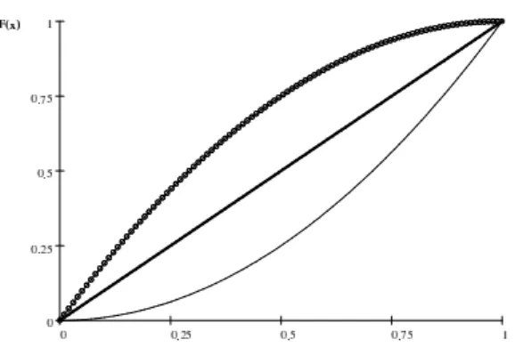
and DB = 1−xˆ. As a robustness check, we here consider two alternative asymmetric
distributions for consumers: Beta(1,2) and Beta(2,1), with F(x; 1,2) = 2x(1−(x/2)) and F(x; 1,2) =x2. In the first case, consumers concentrate more around zero; whereas in the second case, consumers concentrate more around one. Solving for the indifferent consumer, and in turn for the demands, we find that for any given price pair, DA under
the Beta(1,2) distribution is higher than DA under the Beta(1,1) distribution, which
is higher than DA under the Beta(2,1) distribution. The result is rather intuitive,
the more consumers are concentrated around low types which have a low valuation of
9We can think of Apple producing a higher quality good with respect to IBM which in contrast
benefits from a larger network.
Figure 8: Beta(1,1), solid thick line; Beta(2,1), (lower) solid think line; Beta(1,2), (upper) dots line.
quality, the higher the demand for the low quality good. In turn, this affects the results of the model since the demands influence the overall quality differential, measured by k+α(DB−DA)(1−τ). Indeed, the relative weight of the exogenous quality differential
k with respect to the network effect determines the outcome of the full game. Namely, the higher DA, the smaller the high quality firm advantage. Thus, for a given k, it is
more likely for good A to become the good with higher overall quality and to conquer the market.
6.2 Price regions
Given the demands, conditions (1)-(3) can be reduced to: pA−pB< α(1−τ) (2 (pB−pA)−k) (k−2α+ 2ατ) , pB−pA<−α(1−τ) (2 (pB−pA)−k) (k−2α+ 2ατ) +k, pA< α −α 1−τ2+kτ−(pA−pB) (1−τ) (k−2α+ 2ατ) . Assume firstk >2α−2ατ, then we have
pB > α(1−τ) +pA, pB < k−α(1−τ) +pA, pB > pA (k−α+ατ) α(1−τ) − kτ −α 1−τ2 (1−τ)
The lines underlying condition 1 and 2 are parallel and their slope is 1. The intercept of line 1 is smaller than that of line 2. As for condition 3, we have that the intercept is
Figure 9: Price region: k >2α(1−τ).
smaller than the other 2 (and possibly negative) and its slope is higher than 1, therefore, the space defined by these three lines is nonempty and given either by the light grey area or the light and dark grey areas as in Figure 9.
Now assume k <2α(1−τ),then we have
pB< pA+α(1−τ) pB> pA+ (k−α+ατ) pB< α 1−τ2−kτ 1−τ +pA k−α(1−τ) α(1−τ)
The lines underlying condition 1 and 2 are parallel and their slope is 1. The intercept of line 1 is bigger than that of line 2. As for condition 3, we have that the intercept is bigger than the other two and its slope is positive and lower than 1. Therefore, the space defined by these three lines is nonempty and given by the dark grey area as in Figure 10.
6.3 Proofs
6.3.1 Proof of Lemma 1
Let us start by solving the maximization problem of firm B. In the first domain of the profit function, the profit is increasing in the price, as as such, it attains its maximum in the border of the interval in which this branch of the profit is defined, i.e. pB =
pA+α(1−τ). The second branch of the profit function is concave and it attains its
Figure 10: Price region: k <2α(1−τ). relevant domain, i.e. 12(k−α(1−τ)) + pA
2 ≤ pA +α(1−τ), or equivalently pA ≥
k−3α(1−τ) the optimum is pB =pA+α(1−τ).Whenever pA≤k−3α(1−τ), the
optimum is pB = 12(k−α(1−τ)) + p2A. Evidently, given that the optimal solution for
firm depends on whetherpAis superior or inferior tok−3α(1−τ),we must guarantee that
this value is positive. In casek <3α(1−τ), thenpAis always higher thank−3α(1−τ)
and as such, the only relevant best reply for firm B ispB =pA+α(1−τ).
Let us now solve the maximization problem of firm A. In the first domain of the profit function, the profit is increasing in the price, therefore it attains its max-imum in the border of the interval in which this branch of the profit is defined, i.e. pA =pB−(k−α(1−τ)). The second branch of the profit function is concave and it
attains its maximum at pA = 12(pB−α(1−τ)). When 12(pB−α(1−τ)) ∈ (0, pB−
(k−α(1−τ))], or equivalentely, α(1−τ) < pB ≤ 2k−3α(1−τ), the optimum
ob-tains at pA = pB − (k−α(1−τ)), when 12(pB−α(1−τ)) < 0, or equivalently,
pB ≤ α(1−τ) then pA = 0. Finally, when 12(pB−α(1−τ)) > pB −(k−α(1−τ)),
that is, pB >2k−3α(1−τ), the global maximum obtains at pA= 12(pB−α(1−τ)). 6.3.2 Proof of Lemma 2
Consider the situation in which for pB−pA ∈[k−α(1−τ), α(1−τ)] the equilibrium
demand is such that DA ∈(0,1) and DB = 1−DA. Looking at the profit function of
firmB overall it is easy to see that: it is nondecreasing as long aspB< pA+k−α(1−τ),
it has a downward jump to zero atpB =pA+k−α(1−τ), after that it starts increasing
again as long as pB< pA+α(1−τ) and it is zero otherwise. As such, the maximum is
attained atpB=pA+α(1−τ) if this price is lower than the limits imposed by conditions
the price region, which for k <2α(1−τ) is defined by pB < pA+α(1−τ), pB > pA+k−α(1−τ), pB < α 1−τ2−kτ 1−τ +pA k−α(1−τ) α(1−τ) , A similar reasoning applies to firm A.
6.3.3 Proof of Proposition 3 i) 3α3−αk <0
Remember that for 3α−k
3α ≤0, the unique outcome of the price stage is the interior
solution. As such, profits are given by (13) and (14). The revenues are either constant in τi (whenτi < τj) or convex in τi, (when τi > τj). Consequently, the
profit is maximized either at τi = 1 or τi = 0. Therefore overall compatiblity is
eitherτ = 0 orτ = 1.Checking the condition for market coverage (3) it is easy to verify that it does not hold whenever k >3α, given the second stage equilibrium prices and demands, (9), (10), (11) and (12).
ii) α−αk <0< 3α3−αk
In this case, for values of τA, τB ∈ [0,3α3−αk), we have the corner (or the strong
network effect) solution in the price competition stage and profits are given by (15) and (16); and for values of τA, τB∈(3α3−αk,1] we have the interior solution in
the price competition stage, with profits (13) and (14). Let us consider first the revenue function of firm B. If τA ≤ 3α3−αk, as long as τB ≤ τA, firm B’s revenue
is constant and equal to α(1−τA); for τA< τB< 3α3−αk, its revenue is decreasing
inτB and equal toα(1−τB); finally, forτB > 3α3−αk, the revenue is convex inτB.
If τA> 3α3−αk, then, the revenue of firm B is constant and equal to (
α(τA−1)+23k)
2
k−2α(1−τA) ,
as long as τB ≤τA; and convex increasing otherwise. If τA= 1, then the revenue
is constant and equal to 49k. Similarly, for firmA, when τB ≤ 3α3−αk, its revenue is
zero as long as τA≤ 3α3−αk, and positive and convex otherwise. WhenτB > 3α3−αk,
firm A’s revenue is constant and equal to (α(τB−1)+
1 3k)
2
k−2α(1−τB) , as long as τA≤τB; and
convex increasing otherwise. WhenτB = 1, then the revenue is constant and equal
to k
9.
If c = 0, then, firm A always prefers τA = 1, being indifferent in case τB = 1.
τB= 1, otherwise. WhenτA= 1, τB is indifferent. Formally, τB(τA) = 0 ifτA∈ 0,9α9−α4k 1,ifτA∈[9α9−α4k,1) [0,1],ifτA= 1 , τA(τB) = 1,ifτB ∈[0,1) [0,1],ifτB= 1
It is straightforward to see that there are multiple pure strategy Nash equilibria in the compatibility game, namely τA = 1 and τB ∈ [0,1], and τB = 1 and
τA∈
9α−4k
9α ,1
.The overall compatibility level isτ = 1. There is an upward jump in the reaction function of firmB atτA= 9α9−α4k(which is positive fork∈ 2α,94α
, even if it is negative, equilibrium is the same). The overall compatibility level is τ = 1. This equilibrium respects the conditions (1)-(3) for the partition of the parameter space in which it arises.11
If c ∈(0,k
9], we must consider three subsets of (0,k9].12 Let first c < 4k−99α, then
firm B prefersτB = 1 toτB= 0, ifτA≤ 3α3−αk; otherwise, forτA> 3α3−αk she prefers
τB= 0 to τB= 1, if (
α(τA−1)+23k)
2
k−2α(1−τA) > 4k
9 −c. This inequality holds if and only if13 τA>
1 9α
−9c+ (9α−2k) +p(k−9c) (4k−9c)≡τ .e (18) Likewise, firm A prefers τA= 1 to τA= 0, if τB ≤ 3α3α−k; otherwise, if τB > 3α3−αk
she prefersτA= 0 toτA= 1, if and only ifτB >eτ > 3α3−αk. The reaction functions
are, thus, τB(τA) = 1 ifτA∈[0,eτ] 0,ifτA∈[eτ ,1] , τA(τB) = 1 ifτB∈[0,eτ] 0 ifτB∈[τ ,e 1] .
Therefore, there are two asymmetric pure strategy Nash equilibria in the compat-ibility game, namely, (τA, τB) = (1,0) and (τA, τB) = (0,1).Moreover there exists
a unique level ofτi such that firms are indifferent betweenτi = 1 andτi= 0, that
11The market coverage condition is satisfied fork <3α. Whenτ→1, the RHS of condition (3)→ −∞.
Therefore, aspB is finite and positive, the condition always holds.
12We assume that the boundaries of these subsets are positive. In the case in which they are negative,
only the last subset is valid. Nevertheless, results are not affected.
13Define Φ (τ A) = ( α(τA−1)+2 3k) 2 k−2α(1−τA) − `4k 9 −c ´
. Φ (τA) has two real roots,τ+andτ−. It is straightforward to see thatτ−<0< τ+<1.We denoteτ+= 1
9α
“
−9c+ (9α−2k) +p(k−9c) (4k−9c)”≡τe. This is positive forc <α9((4kk−−29αα)).
is τe, defined by (18). Now, let 4k−99α < c < α9 4kk−−29αα, then, if τA < 3α3−αk, firm
B prefersτB = 0 toτB = 1, if α(1−τA) > 49k −c ⇐⇒ τA < 9α−94αk+9c < 3α3−αk;
otherwise, for τA > 3α3−αk, firm B prefers τB = 0 to τB = 1, if τA > eτ. Firm A
prefersτA= 1 to τA= 0, ifτB≤ 3α3α−k; otherwise, ifτB > 3α3−αk she prefersτA= 0
toτA= 1, if and only if τB>τe. The reaction functions are, thus,
τB(τA) = 0 ifτA∈ 0,9α−4k+9c 9α 1 ifτA∈ 9α−4k+9c 9α ,eτ 0 ifτA∈[τ ,e 1] , τA(τB) = 1 if τB ∈[0,eτ] 0 if τB ∈[eτ ,1] .
Then there is a unique asymmetric pure strategy Nash equilibrium in the compat-ibility game, namely, (τA, τB) = (1,0). Also the reaction function of firm B has
two jumps: one upwards atτA= 9α−94αk+9c, and one downwards atτA=eτ. Finally,
let α94kk−−29αα < c < k9, in this case, τ <e 0, and therefore the reaction functions become τB(τA) = 0 ifτA∈ 0,9α−4k+9c 9α 1 ifτA∈ 9α−4k+9c 9α , 3α−k 3α 0 ifτA∈ 3α−k 3α ,1 , τA(τB) = 1 if τB ∈ 0,3α3−αk 0 if τB ∈ 3α−k 3α ,1 .
Notice that, given the increase in the cost with respect to the previous range, both firms start choosing zero compatibility for lower levels of the rival’s choice, (3α3−αk <τe). Then, there is a unique asymmetric pure strategy Nash equilibrium in the compatibility game, namely, (τA, τB) = (1,0). Also the reaction function
of firm B has two jumps: one upwards atτA= 9α−94αk+9c, and one downwards at
τA= 3α3−αk. Independently of the cost subsets, the overall compatibility is τ = 1.
Equilibria, then respect conditions (1)-(3). If c ∈ [k
9,∞), there is a unique symmetric pure strategy Nash equilibrium in
the compatibility game, namely τA = 0 and τB = 0. Both for τA > 3α3−αk and
τA< 3α3−αk, the best reply of firmBis to chooseτB = 0. The overall compatibility
level is τ = 0.This equilibrium respects conditions (1)-(3).
6.3.4 Proof of Proposition 4
Consider the following relevant regions for the parameters:
i) 3α−k
3α <0
When 3α3−αk < 0, the unique equilibrium of the competition stage is the interior equilibrium. Then, the social welfare (17) net of costs is a convex and increasing
function. For high values of c, this function is maximized at τ = 0 and for low values, it is maximized atτ = 1. Nevertheless, as shown in the proof of Proposition 3, these compatibility levels do not comply with markets being covered.
ii) α−αk <0< 3α3−αk
For these range of parameters, the social welfare (17) is defined by: SW = ( 1 2βB+α−cτ,τ ≤ 3α−k 3α βB12 −τ 3−k218α(4−3τ)+9kα2(1−τ)(17−9τ) 18(k−2α+2ατ)2 −cτ,τ > 3α−k 3α
The candidate maxima for this function are: τ = 0,τ = 3α3−αk, orτ = 1. We must, then compare SW(τ = 1) with SW τ = 3α3α−k and with SW (τ = 1). Simple algebra allows us to conclude that
τ = 1 if c < 2 3α τ = 3α−k 3α if 2 3α < c < 3α(4α−5k) + 5k2α 6 (2α−k)2 τ = 0, if c > 3α(4α−5k) + 5k 2α 6 (2α−k)2 .
References
Baake, P. and Boom, A. (2001), “Vertical product differentiation, network externalities, and compatibility decisions”, International Journal of Industrial Organization, 19, 267– 284.
Bala, V. and Goyal S. (2000), “A strategic analysis of network reliability”, Review of Economic Design, 5, 205-228.
Besen, S. and Farrell, J. (1994), “Choosing How to Compete: Strategies and Tactics in Standardization”, Journal of Economic Perspectives, 8, 117-131.
Bloch, F. and Dutta B. (2005), “Communication Networks with Endogenous Link Strenght”, Warwick Economic Research Papers, No 723.
Church, J. and Gandal, N. (1992), “Network effects, software provision, and standard-ization”, Journal of Industrial Economics, 40, 85-103.
Chou, C. and Shy, O. (1993), “Partial compatibility and supporting services”, Eco-nomics Letters, 41, 193-197.
Cr´emer, J. Rey, P. and Tirole J., (2000), “Connectivity in the Commercial Internet”, Journal of Industrial Economics, 48, 433-472.
Farrell, J., Monroe H., and Saloner, G. (1998), “The vertical Organization Of Indus-try: Systems Competition versus Component Competition”, Journal of Economics and
Management Strategy, 7, 143-82.
Grilo, I. Shy, O. and Thisse J. (2001), “Price competition when consumer behaviour is characterized by conformity or vanity” , Journal of Public Economic, 80, 385-408. Katz, M. and Shapiro C., (1985), “Network Externalities, Competition, and Compati-bility”, American Economic Review, 75, 424-440.
Matutes, C. and Regibeau, P. (1988), “Mix and Match: Product Compatibility Without Network Externalities”, Rand Jounal of Economics, 19, 221-234.
Matutes, C., and Regibeau, P. (1992), “Compatibility and bundling of complementary goods in a duopoly”, Jounral of Industrial Economics, 40, 37-54.
Recent titles
CORE Discussion Papers2007/70. Jean GABSZEWICZ, Didier LAUSSEL and Michel LE BRETON. The mixed strategy Nash equilibrium of the television news scheduling game.
2007/71. Robert CHARES and François GLINEUR. An interior-point method for the single-facility location problem with mixed norms using a conic formulation.
2007/72. David DE LA CROIX and Omar LICANDRO. 'The child is father of the man': Implications for the demographic transition.
2007/73. Jean J. GABSZEWICZ and Joana RESENDE. Thematic clubs and the supremacy of network
externalities.
2007/74. Jean J. GABSZEWICZ and Skerdilajda ZANAJ. A note on successive oligopolies and vertical mergers.
2007/75. Jacques H. DREZE and P. Jean-Jacques HERINGS. Kinky perceived demand curves and Keynes-Negishi equilibria.
2007/76. Yu. NESTEROV. Gradient methods for minimizing composite objective function. 2007/77. Giacomo VALLETTA. A fair solution to the compensation problem.
2007/78. Claude D'ASPREMONT, Rodolphe DOS SANTOS FERREIRA and Jacques THEPOT. Hawks
and doves in segmented markets: a formal approach to competitive aggressiveness.
2007/79. Claude D'ASPREMONT, Rodolphe DOS SANTOS FERREIRA and Louis-André
GERARD-VARET. Imperfect competition and the trade cycle: guidelines from the late thirties.
2007/80. Andrea SILVESTRINI. Testing fiscal sustainability in Poland: a Bayesian analysis of cointegration.
2007/81. Jean-François MAYSTADT. Does inequality make us rebel? A renewed theoretical model applied to South Mexico.
2007/82. Jacques H. DREZE, Oussama LACHIRI and Enrico MINELLI. Shareholder-efficient
production plans in a multi-period economy.
2007/83. Jan JOHANNES, Sébastien VAN BELLEGEM and Anne VANHEMS. A unified approach to
solve ill-posed inverse problems in econometrics.
2007/84. Pablo AMOROS and M. Socorro PUY. Dialogue or issue divergence in the political campaign?
2007/85. Jean-Pierre FLORENS, Jan JOHANNES and Sébastien VAN BELLEGEM. Identification and
estimation by penalization in nonparametric instrumental regression.
2007/86. Louis EECKHOUDT, Johanna ETNER and Fred SCHROYEN. A benchmark value for relative
prudence.
2007/87. Ayse AKBALIK and Yves POCHET. Valid inequalities for the single-item capacitated lot sizing problem with step-wise costs.
2007/88. David CRAINICH and Louis EECKHOUDT. On the intensity of downside risk aversion.
2007/89. Alberto MARTIN and Wouter VERGOTE. On the role of retaliation in trade agreements.
2007/90. Marc FLEURBAEY and Erik SCHOKKAERT. Unfair inequalities in health and health care.
2007/91. Frédéric BABONNEAU and Jean-Philippe VIAL. A partitioning algorithm for the network loading problem.
2007/92. Luc BAUWENS, Giordano MION and Jacques-François THISSE. The resistible decline of European science.
2007/93. Gaetano BLOISE and Filippo L. CALCIANO. A characterization of inefficiency in stochastic overlapping generations economies.
2007/94. Pierre DEHEZ. Shapley compensation scheme.
2007/95. Helmuth CREMER, Pierre PESTIEAU and Maria RACIONERO. Unequal wages for equal utilities.
2007/96. Helmuth CREMER, Jean-Marie LOZACHMEUR and Pierre PESTIEAU. Collective annuities
and redistribution.
2007/97. Mohammed BOUADDI and Jeroen V.K. ROMBOUTS. Mixed exponential power asymmetric
conditional heteroskedasticity.
2008/1. Giorgia OGGIONI and Yves SMEERS. Evaluating the impact of average cost based contracts on the industrial sector in the European emission trading scheme.
Recent titles
CORE Discussion Papers - continued
2008/2. Oscar AMERIGHI and Giuseppe DE FEO. Privatization and policy competition for FDI. 2008/3. Wlodzimierz SZWARC. On cycling in the simplex method of the Transportation Problem.
2008/4. John-John D'ARGENSIO and Frédéric LAURIN. The real estate risk premium: A
developed/emerging country panel data analysis. 2008/5. Giuseppe DE FEO. Efficiency gains and mergers.
2008/6. Gabriella MURATORE. Equilibria in markets with non-convexities and a solution to the missing money phenomenon in energy markets.
2008/7. Andreas EHRENMANN and Yves SMEERS. Energy only, capacity market and security of supply. A stochastic equilibrium analysis.
2008/8. Géraldine STRACK and Yves POCHET. An integrated model for warehouse and inventory planning.
2008/9. Yves SMEERS. Gas models and three difficult objectives.
2008/10. Pierre DEHEZ and Daniela TELLONE. Data games. Sharing public goods with exclusion. 2008/11. Pierre PESTIEAU and Uri POSSEN. Prodigality and myopia. Two rationales for social
security.
2008/12. Tim COELLI, Mathieu LEFEBVRE and Pierre PESTIEAU. Social protection performance in
the European Union: comparison and convergence.
2008/13. Loran CHOLLETE, Andréas HEINEN and Alfonso VALDESOGO. Modeling international
financial returns with a multivariate regime switching copula.
2008/14. Filomena GARCIA and Cecilia VERGARI. Compatibility choice in vertically differentiated technologies.
Books
Y. POCHET and L. WOLSEY (eds.) (2006), Production planning by mixed integer programming. New York, Springer-Verlag.
P. PESTIEAU (ed.) (2006), The welfare state in the European Union: economic and social perspectives. Oxford, Oxford University Press.
H. TULKENS (ed.) (2006), Public goods, environmental externalities and fiscal competition. New York, Springer-Verlag.
V. GINSBURGH and D. THROSBY (eds.) (2006), Handbook of the economics of art and culture. Amsterdam, Elsevier.
J. GABSZEWICZ (ed.) (2006), La différenciation des produits. Paris, La découverte.
L. BAUWENS, W. POHLMEIER and D. VEREDAS (eds.) (2008), High frequency financial econometrics: recent developments. Heidelberg, Physica-Verlag.
P. VAN HENTENRYCKE and L. WOLSEY (eds.) (2007), Integration of AI and OR techniques in constraint programming for combinatorial optimization problems. Berlin, Springer.
CORE Lecture Series
C. GOURIÉROUX and A. MONFORT (1995), Simulation Based Econometric Methods. A. RUBINSTEIN (1996), Lectures on Modeling Bounded Rationality.
J. RENEGAR (1999), A Mathematical View of Interior-Point Methods in Convex Optimization.
B.D. BERNHEIM and M.D. WHINSTON (1999), Anticompetitive Exclusion and Foreclosure Through Vertical Agreements.
D. BIENSTOCK (2001), Potential function methods for approximately solving linear programming problems: theory and practice.
R. AMIR (2002), Supermodularity and complementarity in economics. R. WEISMANTEL (2006), Lectures on mixed nonlinear programming.