TI 2010-046/4
Tinbergen Institute Discussion Paper
Efficient Bayesian Estimation and
Combination of GARCH-type Models
David Ardia
1Lennart F. Hoogerheide
21 aeris CAPITAL AG, and University of Fribourg, Switzerland;
Tinbergen Institute
The Tinbergen Institute is the institute for economic research of the Erasmus Universiteit Rotterdam, Universiteit van Amsterdam, and Vrije Universiteit Amsterdam.
Tinbergen Institute Amsterdam Roetersstraat 31
1018 WB Amsterdam The Netherlands
Tel.: +31(0)20 551 3500 Fax: +31(0)20 551 3555 Tinbergen Institute Rotterdam Burg. Oudlaan 50
3062 PA Rotterdam The Netherlands
Tel.: +31(0)10 408 8900 Fax: +31(0)10 408 9031
Most TI discussion papers can be downloaded at http://www.tinbergen.nl.
Efficient Bayesian estimation and combination of
GARCH-type models
∗
David Ardia
†Lennart F. Hoogerheide
‡This version: January 22, 2010
Abstract
This chapter proposes an up-to-date review of estimation strategies avail-able for the Bayesian inference of GARCH-type models. The emphasis is put on a novel efficient procedure named AdMitIS. The methodology automatically constructs a mixture of Student-tdistributions as an approximation to the pos-terior density of the model parameters. This density is then used in importance sampling for model estimation, model selection and model combination. The procedure is fully automatic which avoids difficult and time consuming tuning of MCMC strategies. The AdMitIS methodology is illustrated with an empirical application to S&P index log-returns. Several non-nested GARCH-type models are estimated and combined to predict the distribution of next-day ahead log-returns.
Keywords: GARCH, Bayesian inference, MCMC, marginal likelihood, Bayesian model averaging; adaptive mixture of Student-t distributions, importance sam-pling.
1
Introduction
Volatility forecasting plays an essential role in empirical finance, financial risk man-agement and derivative pricing. Research on modeling volatility dynamics using time series models has been active since the creation of the original ARCH model by En-gle (1982). From there, multiple extensions of the standard ARCH scedastic function have been proposed in order to reproduce additional stylized facts observed in financial markets. These so-calledGARCH-type models recognize that there may be important nonlinearities, asymmetries, and long memory properties in the volatility process; see Bollerslev et al. (1992), Bollerslev et al. (1994) and Engle (2004) for a review. Well ∗Chapter prepared for the book Re-Thinking Risk Measurement, Management and Reporting:
Bayesian Analysis, Expert Elicitation.
†aeris CAPITAL AG Switzerland and University of Fribourg Switzerland;[email protected]
(corresponding author).
‡Tinbergen Institute and Econometric Institute, Erasmus University Rotterdam, The Netherlands; [email protected].
known extensions are the exponential GARCH model by Nelson (1991), the GJR model by Glosten et al. (1993) or the TGARCH model of Zakoian (1994) which ac-count for the asymmetric relation between stock returns and changes in variance (see Black, 1976). In parallel to the development of alternative scedastic functions, numer-ous types of disturbances have been used. The Gaussian and Student-t distributions are common choices while more sophisticated parameterizations such as the skewed Student-t or the mixture of Gaussian distributions allow to model skewness and fat tails in the conditional distribution of returns (see Ausin and Galeano, 2007). More recently, interest has focused on regime-switching GARCH models. In this frame-work, the GARCH parameters are functions of an unobservable state variable and can change over time. These processes provide an explanation of the high persistence in volatility observed with single-regime GARCH models (see, e.g., Lamoureux and Las-trapes, 1990). Furthermore, as shown by Dueker (1997), Klaassen (2002) and Marcucci (2005) for instance, the regime-switching GARCH models allow for a quick change in the volatility level which can lead to significant improvements in risk forecasts.
Until recently GARCH-type models have mainly been estimated using the classical maximum likelihood technique. However, the Bayesian approach offers an attractive alternative. It enables small sample results, probabilistic statements on nonlinear functions of the model parameters, selection and combination of non-nested models. Due to these numerous advantages, the study of GARCH-type models from a Bayesian viewpoint can be considered very promising.
This chapter proposes an up-to-date review of simulation techniques used in the literature to perform the Bayesian estimation of GARCH-type models. The empha-sis is put on a novel approach referred to as AdMitIS. The algorithm constructs a mixture of Student-t distributions to perform an efficient estimation of models via importance sampling. The methodology is fully automatic and has proved to require less computing time for precise estimation results than several well-known alternatives. We describe in some details the steps of the algorithm. In an empirical application to S&P500 index log-returns, we show how it can be used to estimate and combine distribution forecasts of non-nested GARCH-type models.
The chapter proceeds as follows. In Section 2, we survey the existing simulation techniques available for Bayesian GARCH-type models. In Section 3, we present the AdMitIS algorithm. In Section 4, we provide an empirical illustration. Section 5 concludes.
2
Bayesian estimation of GARCH-type models
The maximum likelihood (ML) estimation technique is the most commonly used scheme of inference for GARCH-type models. ML is easy to understand and to imple-ment. Nowadays, several econometric softwares contain a GARCH toolbox and ML estimation of standard GARCH models takes less than one second on a modern com-puter. This is highly desirable for automated trading strategies, for instance, where several models are fitted on thousands of data many times per day. From a theoretical viewpoint, ML estimators benefit from being asymptotically optimal under certain conditions (see Bollerslevet al., 1994; Lee and Hansen, 1994).Despite these appealing features, we face practical difficulties when dealing with the ML estimation of GARCH-type models. First, the maximization of the likelihood function must be achieved via a constrained optimization technique since some (or all) model parameters must be positive to ensure a positive conditional variance. It is also common to require that the covariance stationarity condition holds. This leads to complicated non-linear inequality constraints which render the optimization proce-dure cumbersome. Moreover, the convergence of the optimization is hard to achieve if the true parameter values are close to the boundary of the parameter space and if the GARCH process is nearly non-stationary. Optimization results are often sensitive to the choice of starting values. Second, in standard applications of GARCH models, the interest usually does not center directly on the model parameters but on possi-bly complicated nonlinear functions of the parameters. For instance, a trader might be interested in the unconditional variance implied by a GARCH model, which is a (highly) non-linear function of the model parameters. In order to assess the uncer-tainty of such a quantity, classical inference involves tedious delta methods, simulation from the asymptotic Normal approximation of the parameter estimates or the time-consuming bootstrap methodology. Third, the conditions for the optimal asymptotic properties of ML estimators to hold are fairly difficult to prove, while often assumed to hold in practice. Moreover, since GARCH-type models are highly non-linear, the asymptotic argument would require a very large number of data to hold. This is ob-viously not always the case in practice. Finally, in the case of GARCH with mixture disturbances or regime-switching GARCH models, testing for the number of mixture components or the number of regimes is not possible within the classical framework due to the violation of regularity conditions (see Fr¨uhwirth-Schnatter, 2006, section 4.4).
Fortunately, those difficulties disappear when Bayesian methods are used. First, any constraints on the model parameters can be incorporated in the modeling through appropriate prior specifications. Second, appropriate Markov chain Monte Carlo (MCMC) procedures can explore the joint posterior distribution of the model pa-rameters. These techniques avoid local maxima (i.e., non convergence or convergence to the wrong values) encountered via ML estimation of sophisticated GARCH-type models. Third, exact distributions of nonlinear functions of the model parameters can be obtained at low cost by simulating from the joint posterior distribution. Fourth, the issue of determining the number of mixture components in mixtures disturbances or the number of regimes in regime-switching GARCH model can be addressed by means of marginal likelihoods and Bayes factors. Marginal likelihoods can also be used for model selection and model combination of non-nested GARCH-type models. The latter case is especially interesting in the context of financial risk management since it allows to integrate out model uncertainty, thus accounting for model risk in the forecasts.
The choice of the sampling algorithm is the first issue when dealing with MCMC methods and it depends on the nature of the problem under study. In the case of GARCH-type models, due to the recursive nature of the conditional variance, the joint posterior and the full conditional densities are of unknown forms, whatever as-sumptions are made on the scedastic function or the model disturbances. That is, there exists no conjugate prior under which the parameters’ (conditional) posterior distributions fall within a known class. Therefore, we cannot use the simple Gibbs
sampler and need more elaborated procedures. Hereafter, we shortly present an up-to-date review of the different techniques available to perform the Bayesian estimation of GARCH-type models and discuss their advantages and drawbacks. For a numerical comparison of some of these approaches in the context of GARCH-type models, we refer the reader to Asai (2006) and Ardiaet al. (2009a).
Griddy-Gibbs The Griddy-Gibbs sampler of Ritter and Tanner (1992) is a vari-ant of the Gibbs sampler where each parameter is updated by inversion from the full conditional distribution computed by a deterministic integration rule. The algo-rithm is intuitive and very simple to implement. However, the procedure is extremely time consuming due to the numerical integration steps required at each sweep of the sampler. While this can still be acceptable for simple GARCH specifications, this be-comes a real burden for sophisticated and highly parametrized GARCH-type models. Moreover, for computational efficiency, we must limit the range where the probability mass is computed so that the prior density has to be somewhat informative. In our viewpoint, the Griddy-Gibbs is attractive for its simplicity and remains a useful tool for “one-shot” studies. It is however not relevant in real-world applications, where the models need to be estimated many times on a large number of times series. The Griddy-Gibbs approach is used in the context of GARCH-type models by Bauwens and Lubrano (1998), Bauwens et al. (2000), Bauwens and Lubrano (2002), Wago (2004), Tsay (2005, chapter 10), Ausin and Galeano (2007), Bauwens and Rombouts (2007) and Bauwens et al. (in press).
Importance sampling Importance sampling (IS), due to Hammersley and Hand-scomb (1965), was introduced in econometrics and statistics by Kloek and van Dijk (1978). The IS approach relies on an importance density which approximates the posterior density of the model parameters. Draws are generated from an importance density and weighted, with higher weights given to draws for which the importance density is relatively small compared with the posterior. Then, quantities of interest of the posterior distribution (or predictive distribution) are estimated by weighted aver-ages of (functions of) draws. This methodology leads to a fast estimation since it only requires generating and weighting draws. Moreover, it generates uncorrelated draws so that the whole posterior sample can be used for Bayesian inference (i.e., no burn-in or ‘thinning’), and so that the precision of the estimators is easily assessed. However, the key issue for applicability and efficiency is the choice of the importance density. Finding this can be a bit of an art, especially if the posterior density is asymmetric or multi-modal. For instance, in the case of a GARCH model with mixture distur-bances, the posterior distribution is multimodal. In this case, a (standard) unimodal importance density may imply that some draws have huge weights leading to large inefficiencies in the estimation, or worse, that relevant parts of the parameters space are completely ‘missed’. The importance distribution should be close to the posterior distribution and it is especially important that the tails of the importance should not be thinner than those of the posterior. Bayesian estimation of GARCH-type mod-els using importance sampling is proposed by Geweke (1988), Geweke (1989b) and Kleibergen and van Dijk (1993).
Metropolis-Hastings The Metropolis-Hastings (MH) algorithm was introduced by Metropoliset al.(1953) and generalized by Hastings (1970). The approach constructs a Markov chain by generating draws from acandidate density; the candidate draw is then accepted (or rejected) based on an acceptance probability. If the candidate is accepted, the chain moves to the new value, otherwise the chain stays in the current state. After a burn-in period, which is required to make the influence of initial values negligible, draws from the Markov chain are considered as (correlated) draws from the joint posterior distribution of interest. Two variants of the MH approach are most common: (i) the independence chain MH and (ii) the random-walk MH. In the former case, candidate draws are generated from an unconditional candidate distribution whereas in the latter draws are generated from a distribution conditional on (and around) the current value of the chain. In both variants the candidate distribution must be tuned to achieve a reasonable acceptance rate and to explore sufficiently the domain of the posterior distribution. This tuning process requires preliminary runs and some knowledge of MCMC techniques from the user. Hence, the method is not automatic which is not a desirable property. In addition, for interpreted languages such as R (R Development Core Team, 2009) or MATLAB°c (The MathWorks Inc., 2009), the MH
algorithm can be significantly slower than the importance sampling strategy. This is so because the probability of acceptance of the new draw depends on the current state of the Markov chain; hence, the algorithm cannot be vectorized. Finally, the MH algorithm creates a sequence of correlated draws from the posterior distribution. Therefore, robust techniques must be used to assess the precision of the estimators and more draws are required to achieve the same degree of (numerical) precision as the IS approach. The MH algorithm is used in the context of GARCH-type models by M¨uller and Pole (1998), Vrontos et al. (2000), Tsay (2005, chapter 10), Gerlach and Chen (2006), Miazhynskaia and Dorffner (2006), Aussenegg and Miazhynskaia (2006), Miazhynskaia et al. (2006), Chen et al. (2008), Chen and Gerlach (2008) and Chen
et al. (in press).
An interesting strategy has been proposed to automate the MH algorithm and improve its efficiency. This approach is proposed by Nakatsuma (1998, 2000) and consists of an independence chain MH algorithm where the proposal distributions are constructed from auxiliary ARMA processes on the squared observations. In addition to be fully automatic and more efficient than naive MH approaches, the methodology can be extended to regime-switching GARCH models; see Ardia (2008b, chapter 7) and Ardia (2009a). Note however that the construction of the proposal distributions highly depends on the form of the scedastic function and is not applicable to all GARCH-type models. Moreover, the algorithm requires filtering steps which significantly increase the computational burden for highly parametrized models. The approach of Nakatsuma (1998, 2000) is used in Nakatsuma and Tsurumi (1999), Kaufmann and Fr¨uhwirth-Schnatter (2002), Kaufmann and Scheicher (2006), Rachev et al. (2008, chapter 11), Hennekeet al.(2009), Ardia (2008b) and Ardia (2009a). The algorithm is implemented in theRpackagebayesGARCH(Ardia, 2008a, 2009b) for the GARCH(1,1) model with Student-t disturbances.
AdMitIS Recently, Ardia et al.(2009a) and Ardia et al. (2009c) relied on a special case of the adaptive approach proposed by Hoogerheide (2006); Hoogerheide et al.
method-ology, named AdMitIS for importance sampling with adaptive mixture of Student-t distributions, consists of two steps. First, the algorithm fits adaptively a mixture of Student-t distributions to the kernel of the posterior density. Then, importance sam-pling is used to obtain quantities of interest for the target posterior distribution, using the fitted mixture as the importance density. The estimation procedure is fully auto-matic. Moreover, Ardia et al. (2009a) compared the methodology to standard cases of IS and MH algorithm using a naive candidate and to the Griddy-Gibbs approach. Overall, they demonstrate the superiority of the AdMitIS approach both in terms of efficiency and reliability.
Due to its flexibility, the adaptive algorithm is able to provide a suitable importance distribution for non-elliptical, possibly multi-modal, posterior distributions. But it is not only useful for sophisticated GARCH-type models. For large samples and/or simple scedastic specifications, the posterior distribution of the model parameters is likely to be roughly elliptical. In these cases, the adaptive approach will stop with one or two mixture components, leading to a simple unimodal symmetric importance density. The adaptive fitting together with the importance sampling estimation is achieved fairly quickly. Therefore, models can be re-estimated many times on many data sets without practical issues. This is clearly an appealing aspect for practitioners. Moreover, Ardia et al.(2009c) show that the approach allows an efficient and reliable estimation of marginal likelihood, which lies at the heart of model selection and model combination. The approach can therefore be used to estimate, select and combine GARCH-type models in a simple, quick and efficient fashion.
3
Adaptive mixture of Student-
t
method
The adaptive mixture of Student-t distributions (AdMit) procedure has been de-veloped by Hoogerheide (2006); Hoogerheide et al. (2007); see also Hoogerheide and van Dijk (2008). The AdMit methodology consists of the construction of a mix-ture of Student-t distributions which approximates a target distribution of interest. The fitting procedure relies only on a kernel of the target density, so that the nor-malizing constant is not required. In a second step this approximation is used as an importance function in importance sampling (AdMitIS) or as a candidate den-sity in the independence chain MH algorithm (AdMitMH). Both AdMitIS and Ad-MitMH strategies have been implemented in the R package AdMit (Ardia et al., 2008) and is freely available from the Comprehensive R Archive Network (CRAN)
at http://cran.r-project.org/package=AdMit. The usage of the package with
empirical examples is discussed in Ardiaet al. (2009a) and Ardia et al. (2009b). Hoogerheide et al. (2007) mention several reasons why mixtures of Student-t dis-tributions are natural importance or candidate disdis-tributions. Indeed, a Student-t mixture
• provides an accurate approximation to a wide variety of target distributions, with substantial skewness and high kurtosis; it can deal with multi-modality and with non-elliptical shapes.
• has fatter tails than the Normal distribution (especially if one specifies Student-t components with few degrees of freedom). Therefore, the risk is small that the tails of the importance or candidate are thinner than those of the target distribution.
Moreover, from a purely theoretical framework, mixture of Student-t densities can approximate any density function to arbitrary accuracy under certain conditions (Zeevi and Meir, 1997).
The AdMit methodology can be used in different contexts. For a general and detailed presentation, we refer the reader to Ardiaet al.(2009b). Here, we concentrate on the Bayesian estimation of GARCH-type models with importance sampling.
Because of its superiority compared to several alternative methods, both in terms of efficiency and reliability of posterior estimation (Hoogerheide, 2006; Hoogerheide
et al., 2007; Ardia et al., 2009a) and of marginal likelihood estimation (Ardia et al., 2009c), we will make use of the AdMitIS approach.
For a given GARCH-type model, we denote by θ∈Θ⊆Rd the vector of parame-ters, p(θ|y) the posterior density of θ and y= (y. 1, . . . , yT)0 the vector of log-returns. The joint posterior density ofθ is then obtained by Bayes’ theorem as
p(θ|y) = R p(y|θ)p(θ)
Θp(y|θ)p(θ)dθ
, (1)
where p(y|θ) is the joint density of y given θ and p(θ) is the exact prior density of
θ, i.e., not merely a prior kernel. In expression (1), we define k(θ) =. p(y|θ)p(θ) as the kernel function of the joint posterior and
p(y)=. Z
Θ
k(θ)dθ (2)
as the marginal likelihood. It is clear that the marginal likelihood is equal to the nor-malizing constant of the joint posterior density. As the key ingredient in Bayes factors, the marginal likelihood lies at the heart of model selection and model combination in Bayesian statistics (see, e.g. Kass and Raftery, 1995).
The AdMit methodology constructs a mixture of Student-t distributions in order to approximate the posterior density p(θ|y). The density of a mixture of Student-t distributions can be written as
q(θ) = H X h=1
ηhtd(θ|µh,Σh, ν),
where {ηh} are the mixing probabilities of the Student-t components (0 6 ηh 6 1 andPHh=1ηh = 1) andtd(θ|µh,Σh, ν) is a d-dimensional Student-tdensity with mode vectorµh, scale matrix Σh, andν degrees of freedom. The adaptive mixture approach determines H, {ηh}, {µh} and {Σh} based on the kernel k(θ). It consists of the following steps:
Step 0 Compute the mode µ1 and scale Σ1 of the first Student-t distribution in the
mixture as µ1 = arg maxθ∈Θlogk(θ), the mode of the log kernel function, and
ofN points {θ[i]}from this first stage candidate densityq(θ) = td(θ|µ1,Σ1, ν),
with small ν to allow for fat tails. N is typically a very large number, e.g., N = 100 000.
After that add iteratively components to the mixture by performing the following steps:
Step 1 Compute the importance sampling weights w(θ[i])=. k(θ[i])
q(θ[i]) (3) for i = 1, . . . , N. In order to determine the number of components H of the mixture, we make use of a simple diagnostic criterion: thecoefficient of variation, i.e., the standard deviation divided by the mean, of the importance sampling weights {w(θ[i])}. If the relative change in the coefficient of variation of the importance sampling weights caused by adding one new Student-tcomponent to the candidate mixture is small, e.g., less than 10%, then the algorithm stops and the current mixture q(θ) is the approximation. Otherwise, the algorithm goes to step 2.
Step 2 Add another Student-t distribution with density td(θ|µh,Σh, ν) to the cur-rent mixture. Since for most GARCH-type specifications the region of integration Θ is bounded, it may occur that w(θ) attains its maximum at a boundary of Θ. In this case, minus the inverse Hessian of logw(θ) evaluated at its mode (which would otherwise provideµh and Σh) may be a very poor choice; in fact this Hessian may not even be positive definite. Therefore, in order to avoid any numerical problem, µh and Σh are obtained as the estimated mean and covari-ance based on a subset of draws corresponding to a certain percentage of largest weights. More precisely, µh and Σh are obtained as
µh =X j∈Jc w(θ[j]) P j∈Jcw(θ[j]) θ[j], Σh =X j∈Jc w(θ[j]) P j∈Jcw(θ[j]) (θ[j]−µh)(θ[j]−µh)0,
whereJc denotes the set of indices corresponding to thecpercents of the largest weights using the sample{w(θ[j)}fromq(θ) we already have. Since our aim is to detect regions with relatively too little candidate probability mass as compared with the target distribution (e.g., a distant mode), the percentagec is typically a low value, i.e., 5%.
The new component is based on the ratio of the previous mixture of Student-t densities and the target density kernel k(θ|y). It is located where this ratio is
relatively high, which does not depend on the normalizing constant of the target density.
Step 3 Choose the probabilities {ηh}in the mixture q(θ) = PH
h=1ηhtd(θ|µh,Σh, ν) by minimizing the coefficient of variation of the importance sampling weights.
Step 4 Draw a sample of N points {θ[i]} from the new mixture of Student-t distri-butionsq(θ) = PHh=1ηhtd(θ|µh,Σh, ν) and go to Step 1.
The coefficient of variation of the importance sampling weights is a natural and intuitive measure of quality of the candidate as an approximation to the target. If the candidate and the target distributions coincide, all importance sampling weights are equal, so that the coefficient of variation is zero. For a poor candidate that not even roughly approximates the target, some importance sampling weights are huge while most are (almost) zero, so that the coefficient of variation is high. The better the candidate approximates the target, the more evenly the weight is divided among the candidate draws, and the smaller the coefficient of variation of the importance sampling weights. We refer the reader to Ardia et al. (2009a) for theoretical reasons justifying the coefficient of variation.
The mode and Hessian of the log kernel function (step 0), the coefficient of variation of the IS weights (steps 1 and 3), and the scaled IS weightsw(θ[j])/Pj∈Jcw(θ[j]) (step 2) do not depend on the normalizing constant of the target density, which explains why the whole AdMit procedure only requires a target densitykernel.
Once the adaptive mixture of Student-t distributions has been fitted to the target density p(θ|y) through the kernel function k(θ), the approximation q(θ) is used in importance sampling to obtain quantities of interest of the posteriorp(θ|y) or perform model selection and model combination. The importance sampling technique is based on the relationship Ep £ g(θ)¤= R ΘRg(θ)p(θ|y)dθ Θp(θ|y)dθ = R ΘRg(θ)w(θ)q(θ)dθ Θw(θ)q(θ)dθ = Eq £ g(θ)w(θ)¤ Eq £ w(θ)¤ , (4) whereg(θ) is a given function (integrable with respect top(θ|y)),Ep denotes the ex-pectation with respect to the posterior densityp(θ|y) andEq denotes the expectation with respect to the Student-t mixture q(θ). The importance sampling estimator of Ep £ g(θ)¤ is given by ˆ Ep £ g(θ)¤ = PL l=1Pg(θ[l])w(θ[l]) L l=1w(θ[l]) , (5)
where {θ[l]} is a sample of L i.i.d. draws from the importance density q(θ). Under
certain conditions, ˆEp is a consistent estimator ofEp (see Geweke, 1989a). The choice of the function g(θ) allows to obtain different quantities of interest; for instance, the posterior mean is obtained withg(θ)=. θ and the posterior probability of a setS⊆Rd is obtained with g(θ)= 1. {θ∈S}, where 1{·} denotes the indicator function.
As for any time series model, prediction is essential. The Bayesian framework allows for obtaining predictive densities that by construction incorporate parameter uncertainty when forecasting future observations. For instance, the one-step ahead predictive density is obtained by setting g(θ) to the density of the one-step ahead observation yT+1 in expression (4). Formally,
p(yT+1|y) =
Z
Θ
This quantity is easily estimated using (5) sincep(yT+1|θ,y) is known in closed-form
for any GARCH-type model. For multi-step ahead forecasts, the predictive density is of unknown form and we must rely on simulation in conjunction with the method of composition. We refer the reader to Ardia (2008b, chapter 6) for an illustration.
The Bayesian framework is also appealing for selecting and combining models, which is achieved through the computation of the posterior model probability. As-sume that we have M (possibly non-nested) GARCH-type models Mi with marginal likelihoodpi(y) and prior model probabilityp(Mi). Usually, the prior model probabil-ity is equal for all models or favors parsimonious specifications. The posterior model probability of model Mi is then given by
p(Mi|y) =
pi(y)p(Mi) PM
i=1pi(y)p(Mi) ,
where the importance sampling approach immediately provides the estimator for the marginal likelihood pi(y) ˆ pi(y) = 1 L L X l=1 wi(θ[il]), (7) as shown by Kloek and van Dijk (1978) for instance. In expression (7), wi(θi) denotes the weight function (3) based on the kernelki(θi) and the Student-t mixture density qi(θi) corresponding to model Mi, and {θi[l]}are L i.i.d. draws generated fromqi(θi), where θi ∈Θi ⊆ Rdi. For model discrimination, the model with the largest posterior probability will then be selected. The posterior probability can can also be used to produce a combination of the predictive distributions, an approach referred to as Bayesian model averaging (BMA) in the literature (see Kass and Raftery, 1995). For instance, the one-step ahead BMA predictive density is given by
pBMA(yT+1|y) =
M X
i=1
pi(yT+1|y)p(Mi|y), (8) wherepi(yT+1|y) denotes the predictive density of modelMi, which is easily obtained using (6) with the densitypi(yT+1|θi,y) and the posteriorpi(θi|y) corresponding to Mi. Expression (8) is nothing else than the weighted average of the M single-model one-step ahead predictive densities, where the weights are the posterior model proba-bilities. This distribution of the one-step ahead observation accounts for uncertainty on both parameter values and model choice.
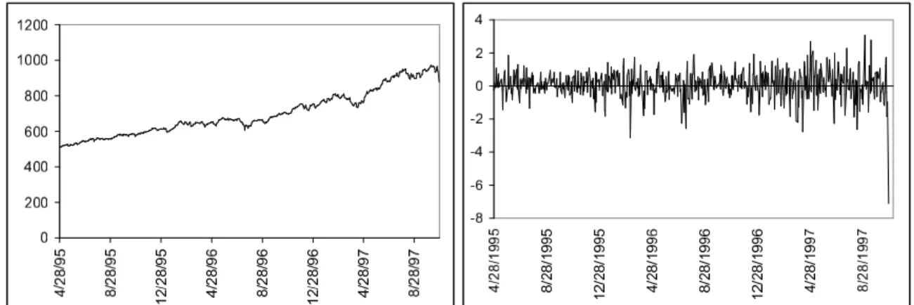
Figure 1: Data: S&P500 index and log-returns (expressed in percent).
4
Empirical illustration
This section proposes an illustration of the AdMitIS strategy with the Bayesian estimation of two non-nested GARCH-type models. The posterior model probabilities are estimated and used to combine the predictive densities of the one-day ahead log-returns. This case study aims at describing in a real-life example the mechanics of the AdMitIS strategy and demonstrating its effectiveness.
We apply our Bayesian estimation methods to daily observations of the S&P500 index log-returns. The sample period is from April 28 1995 to October 27 1997, for a total of 633 observations. The reason for this particular data window of 2.5 years, which is long enough to estimate GARCH-type models, is that it ends with an extremely negative return, which makes the differences between forecasts from the two models more clearly visible. Further, for this data set the typically imposed restrictions on the models (for ensuring stationarity and positivity of the volatility process) seem to be supported by the data. The analysis of the correctness of the model restrictions falls outside the scope of this chapter. The time series has been demeaned and the nominal returns are expressed in percent. Robust autocorrelation tests do not exhibit any autocorrelation in the returns, whereas significant autocorrelation is detected for the squared log-returns, thus suggesting GARCH effects in the data.
The two models are based on two non-nested scedastic functions. For the variance dynamics, we use the parsimonious but effective GJR(1,1) and EGARCH(1,1) specifi-cations. These models are well-known in univariate GARCH modeling for their ability to reproduce the asymmetric behavior of the conditional variance observed in equity markets. For the model disturbances, we consider Student-t innovations, which allow to reproduce fat tails in the conditional distributions.
Formally, the log-returns {yt} can be expressed as yt=σt% εt where the scedastic function σt can be of either type:
GJR σ2 t . =ω+α y2 t−1+γ yt2−11{yt−1<0}+β σt2−1 (ω >0, α, γ, β ≥0) EGARCH log(σ2
and where the disturbances εt are i.i.d. Student-t variates: p(εt)=. Γ¡ν+1 2 ¢ Γ¡ν 2 ¢ (πν)1/2 µ 1 + ε2t ν ¶−ν+1 2 (ν > 2). The scalar % is a normalizing factor
q ν−2
ν to ensure that the conditional variance is σ2
t. For the Student-t variates yt−1/σt−1 that are normalized to have variance 1 the
expectationE(|yt−1/σt−1|) is given by:
E(|yt−1/σt−1|) =
√
ν−2 Γ((ν−1)/2) √
π Γ(ν/2) .
Note the positivity constraints on the model parameters in order to ensure a pos-itive conditional variance and the constraint on the degrees of freedom parameter to ensure the existence of a finite conditional variance. Moreover, we require the process to be covariance stationary, i.e.α+γ/2+β <1 for the GJR(1,1) model and|β|<1 for the EGARCH(1,1) model. Note that the model specifications are used for illustrative purposes only; checking for possible model misspecification is beyond the scope of the present paper.
For both models we specify weakly informative, proper prior distributions on the parameters that can roughly be interpreted as the proper versions of the improper priors used by Vrontos et al.(2000), where we use proper priors for computing poste-rior model probabilities and performing Bayesian model averaging. For the GJR(1,1) model, we specify a normal distribution for log(ω) (with mean log(0.01) and standard deviation log(10)), which amounts to a 95% prior interval for ω between 0.0001 and 1. For α, γ and β we use a uniform prior on the subspace with α > 0, γ >0, β > 0, α+γ/2 +β <1. We specify an exponential prior distribution with mean 20 for ν−2. For the EGARCH(1,1) model we choose a uniform prior on [-1,1] for β. For ω,α and γ we use normal priors with mean 0 and standard deviation 0.1. Again we specify an exponential prior distribution with mean 20 for ν−2.
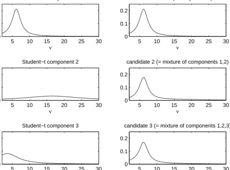
The priors are combined with the likelihood function, leading to the posterior kernel functions. These kernels are used in the AdMit algorithm. For each model, AdMit was applied withN = 100 000 draws. For both models, the algorithm led to a mixture of three Student-t distributions as the candidate distribution. Figure 2 illustrates the steps of the AdMit algorithm for the marginal posterior ofν in the EGARCH model. The first candidate is a Student-t distribution around the posterior mode. Second, a Student-t component is added that is located in the right tail, yielding a right-skewed candidate. This consists of a substantial improvement of the approximation to the posterior, shown in Figure 4, so that the AdMit algorithm continues. Third, a Student-t component is added that is placed in the short left tail. This is only a minor improvement of the candidate, so that the AdMit algorithm stops at three components. Notice that the AdMit algorithm provides an approximation of the joint posterior in the 5-dimensional parameter space; Figure 2 shows the 1-dimensional marginal candidate distribution of ν only for illustration.
5 10 15 20 25 30 0 0.1 0.2 ν Student−t component 1 5 10 15 20 25 30 0 0.1 0.2 ν candidate 1 (= component 1) 5 10 15 20 25 30 0 0.1 0.2 ν Student−t component 2 5 10 15 20 25 30 0 0.1 0.2 ν
candidate 2 (= mixture of components 1,2)
5 10 15 20 25 30 0 0.1 0.2 ν Student−t component 3 5 10 15 20 25 30 0 0.1 0.2 ν
candidate 3 (= mixture of components 1,2,3)
Figure 2: The AdMit algorithm automatically and iteratively approximates the skewed shapes of the marginal posterior ofν in the EGARCH model.
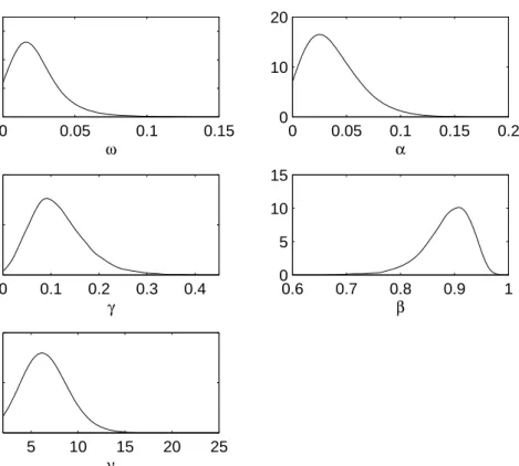
Bayesian estimation results from the AdMit-IS approach are reported in Table 1. Estimates of the marginal posterior densities are shown in Figures 3 and 4. We notice the strong evidence for the leverage effect in the time series (γ > 0 in GJR, γ < 0 in EGARCH), as well as conditional leptokurticity in the data (rather small ν). We also report the numerical standard errors (i.e., the square root of the variance of the estimates that can be expected if the simulations were to be repeated with different random numbers). The RNE is the relative numerical efficiency of the estimate, i.e., the ratio between an estimate of the variance of a hypothetical estimator based on direct sampling and the importance sampling estimator’s estimated variance with the same number of draws. RNE is an indicator of efficiency of the chosen importance function; if the target and importance densities coincide, RNE equals one, whereas a very poor importance density will have a RNE close to zero. Both NSE and RNE are estimated by the method given in Geweke (1989a). The numerical standard error and relative numerical efficiency indicate a reasonable degree of efficiency for the methods, which may be difficult to achieve for non-elliptical, skewed, multidimensional poste-rior distributions. Table 2 shows estimation results from IS using a naive candidate, a Student-t distribution around the posterior mode. Note the lower RNE for all co-efficients in both models, as compared with AdMit-IS. For the GJR parameter ω and EGARCH parameter ν, for which the marginal posteriors are substantially skewed, the RNEs are 3.4 and 2.6 times higher in the AdMit-IS approach. Further, note the lower estimate of the posterior standard deviation of the EGARCH parameterν. Even after 100000 draws, the naive approach may hardly cover some relevant regions of the parameter space.
As explained in the previous Section, the AdMit algorithm also delivers a suitable importance density for marginal likelihood estimation. The natural logarithm of the AdMit-IS estimate of the marginal likelihood is given by -725.6930 and -724.5382 for the GJR and EGARCH model, respectively. This implies a Bayes factor of 3.1734 in favor of the EGARCH model. Under equal prior model probabilities, i.e., a prior odds ratio of 1, the posterior probabilities for the GJR and EGARCH models are estimated as 0.2396 and 0.7604, respectively.
M1: GJR Student-t M2: EGARCH Student-t
θ Eˆp(θ) NSE RNE Vˆ1p/2(θ) θ Eˆp(θ) NSE RNE Vˆ1p/2(θ)
ω 0.0205 0.0002 0.0927 0.0147 ω -0.0105 0.0001 0.1198 0.0117
α 0.0349 0.0002 0.1232 0.0240 α 0.1384 0.0002 0.2525 0.0367
γ 0.1124 0.0005 0.1404 0.0566 γ -0.0737 0.0002 0.2230 0.0318
β 0.8898 0.0004 0.1207 0.0424 β 0.9733 0.0002 0.1201 0.0201
ν 6.4843 0.0201 0.0693 1.6745 ν 6.6905 0.0140 0.1844 1.9667
Table 1: Posterior results for the two non-nested models using AdMit-IS. ˆEp(θ) pos-terior mean estimate. NSE: numerical standard error of the pospos-terior mean esti-mate. RNE: relative numerical efficiency of the posterior mean estimate; ˆV1p/2(θ): posterior standard deviation estimate. The number of importance sampling draws is L= 100 000.
M1: GJR Student-t M2: EGARCH Student-t
θ Eˆp(θ) NSE RNE Vˆ1p/2(θ) θ Eˆp(θ) NSE RNE Vˆ1p/2(θ)
ω 0.0202 0.0003 0.0271 0.0148 ω -0.0106 0.0001 0.0608 0.0117
α 0.0350 0.0003 0.0890 0.0241 α 0.1389 0.0003 0.1722 0.0372
γ 0.1112 0.0008 0.0516 0.0565 γ -0.0734 0.0002 0.1710 0.0318
β 0.8903 0.0006 0.0427 0.0424 β 0.9732 0.0003 0.0467 0.0202
ν 6.5077 0.0291 0.0337 1.6884 ν 6.6508 0.0180 0.1028 1.8265
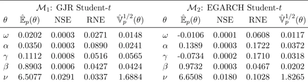
Table 2: Posterior results for the two non-nested models using naive IS (i.e., using a Student-t candidate distribution around the posterior mode). ˆEp(θ) posterior mean estimate. NSE: numerical standard error of the posterior mean estimate. RNE: rela-tive numerical efficiency of the posterior mean estimate; ˆV1p/2(θ): posterior standard deviation estimate. The number of importance sampling draws is L= 100 000.
0 0.05 0.1 0.15 0 10 20 30 ω 0 0.05 0.1 0.15 0.2 0 10 20 α 0.6 0.7 0.8 0.9 1 0 5 10 15 β 0 0.1 0.2 0.3 0.4 0 5 10 γ 5 10 15 20 25 0 0.1 0.2 ν
Figure 3: Marginal posterior densities for parameters in GJR model.
−0.1 −0.05 0 0.05 0 20 ω 0 0.1 0.2 0.3 0 5 10 15 α 0.8 0.85 0.9 0.95 1 0 10 20 30 β −0.2 −0.1 0 0.1 0 10 20 γ 5 10 15 20 25 30 0 0.1 0.2 ν
0 1 2 3 4 5 6 0 0.2 0.4 0.6 0.8 1 1.2 1.4
σ
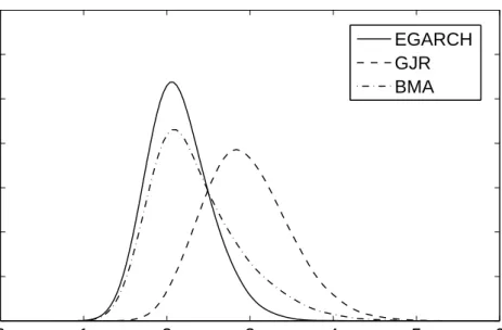
T+1 EGARCH GJR BMAFigure 5: Predictive density of σT+1 for EGARCH model, GJR model and Bayesian
Model Averaging of the two models.
−10 −5 0 5 10 0 0.05 0.1 0.15 0.2 0.25
y
T+1 EGARCH GJR BMAFigure 6: Predictive density of yT+1 for EGARCH model, GJR model and Bayesian
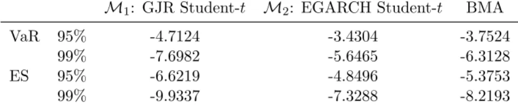
M1: GJR Student-t M2: EGARCH Student-t BMA
VaR 95% -4.7124 -3.4304 -3.7524
99% -7.6982 -5.6465 -6.3128
ES 95% -6.6219 -4.8496 -5.3753
99% -9.9337 -7.3288 -8.2193
Table 3: Estimates of the Value at Risk and Expected Shortfall for the GJR model, EGARCH model, and Bayesian Model Averaging of the two models.
In Figures 5 and 6 we display the predictive densities for the volatility σT+1 and
log-return yT+1 for the date October 28 1997, for the GJR and EGARCH models as
well as for Bayesian Model Averaging (BMA) which combines the predictive densities from the models via the posterior model probabilities. Approximate values of risk measures such as the VaR and ES can be read from the figure.
We compute the IS estimator V aR[IS of the 100α% one-day-ahead Value at Risk (VaR) as follows. First, L draws θ[l] are simulated from the candidate, and the
cor-responding importance weights w(θ[l]) are computed. Second, for the ˜L ( ˜L ≤ L)
draws θ[l] with non-zero weights w(θ[l]) a log-return y[l]
T+1 is simulated from its
distri-bution given the model and parameter values θ[l]. Third, the simulated log-returns
yT[l]+1 are sorted ascending as yT(i+1) (i = 1, . . . ,L) and the VaR is estimated as˜ yT(k+1) with Sk = 1−α where Sk ≡
Pk
j=1w(θ˜ (i)) is the cumulative sum of scaled weights
˜
w(θ(j))≡ w(θ(j))
PL˜
i=1w(θ(i))
(scaled to add to 1) corresponding to the ascending log-returns. In general there will be no k such that Sk = 1−α, so that one interpolates between the values ofy(Tk+1) and yT(k+1+1) whereSk+1 is the smallest value with Sk+1 >1−α. The
IS estimatorEScIS of the 100α% Expected Shortfall (ES) is subsequently computed as c
ESIS = Pk
j=1w∗(θ(j))y (j)
T+1, the weighted average of the k values y (j)
T+1 (j = 1, . . . , k)
with weights w∗(θ(j)) ≡ w(θ(j)) Pk
i=1w(θ(i)) (adding to 1). For IS estimation of VaR and ES
in case of more general profit/loss functions see Hoogerheide and Van Dijk (2010). Hoogerheide and Van Dijk (2010) also introduce an additional approximation step, targeted particularly on generating high loss scenarios, that can make the simulation-based estimation of VaR and ES even more efficient.
Table 3 displays the values for the one-day-ahead VaR and ES for October 28 1997, for both models and BMA. Figures 5 and 6 and Table 3 show that the GJR model predicts higher risk than EGARCH, with BMA results naturally taking a position in between. Accounting for both the uncertainty on estimated parameters and the uncertainty on model choice, we obtain BMA estimates of VaR and ES (at the 95% risk level) at -3.7524 and -5.3753.
5
Conclusion
The study of GARCH-type models from a Bayesian viewpoint is relatively recent and can be considered very promising due to the advantages of the Bayesian approach compared to classical techniques. In particular, the Bayesian framework enables small sample results, robust estimation, probabilistic statements on nonlinear functions of the model parameters and model discrimination. Moreover, the Bayesian paradigm allows to combine model forecasts, thus accounting for model risk in the predictions, which is crucial from a risk management perspective.
This chapter reviewed existing methods for the Bayesian estimation of GARCH-type models. We focused our presentation on a novel approach, named AdMitIS, which performs importance sampling with an adaptive mixture of Student-t distribution as the importance distribution. The methodology allows a quick and efficient estimation of any kind of GARCH-type models. Moreover, with this approach, it is easy to com-bine forecasts of non-nested models. The estimation procedure is fully automatic and is achieved within a reasonable computational time compared to alternative MCMC techniques. This is of primary importance for automated trading systems for instance, where models are estimated frequently and for numerous datasets.
The AdMitIS algorithm was described in details and we provided an application to S&P500 index log-returns. We illustrated how four non-nested GARCH-type models could be estimated and combined in order to forecast the next-day ahead log-returns distribution.
In a next study, we plan to investigate the performance of the Bayesian model averaging approach when forecasting standard risk measures such as the value-at-risk and the expected shortfall.
References
Ardia D (2008a). ‘bayesGARCH’: Bayesian Estimation of the GARCH(1,1) Model with Student-t Innovations in R. URL http://CRAN.R-project.org/package=
bayesGARCH.
Ardia D (2008b). Financial Risk Management with Bayesian Estimation of GARCH Models: Theory and Applications, volume 612 of Lecture Notes in Economics and Mathematical Systems. Springer-Verlag, Berlin, Germany. ISBN 978-3-540-78656-6. doi:10.1007/978-3-540-78657-3.
Ardia D (2009a). “Bayesian Estimation of a Markov-Switching Threshold Asymmetric GARCH Model with Student-t Innovations.” Econometrics Journal, 12, 105–126. doi:10.1111/j.1368-423X.2008.00253.x.
Ardia D (2009b). “Bayesian Estimation of the GARCH(1,1) Model with Student-t Innovations in R.” MPRA working paper. URL http://mpra.ub.uni-muenchen.
Ardia D, Hoogerheide LF, van Dijk HK (2008). ‘AdMit’: Adaptive Mixture of Student-t DisStudent-tribuStudent-tions for EfficienStudent-t SimulaStudent-tion in R. URL http://CRAN.R-project.org/
package=AdMit.
Ardia D, Hoogerheide LF, van Dijk HK (2009a). “Adaptive Mixture of Student-t Distributions as a Flexible Candidate Distribution for Efficient Simulation: The R Package AdMit.” Journal of Statistical Software, 29(3), 1–32. URL http://www.
jstatsoft.org/v29/i03/.
Ardia D, Hoogerheide LF, van Dijk HK (2009b). “AdMit: Adaptive Mixtures of Student-t Distributions.” The R Journal, 1(1), 25–30.
Ardia D, Hoogerheide LF, van Dijk HK (2009c). “To Bridge, to Warp or to Wrap? A Comparative Study of Monte Carlo Methods for Efficient Evaluation of Marginal Likelihoods.” Tinbergen Institute report 09-017/4.
Asai M (2006). “Comparison of MCMC Methods for Estimating GARCH Models.”
Journal of the Japan Statistical Society, 36(2), 199–212.
Ausin MC, Galeano P (2007). “Bayesian Estimation of the Gaussian Mixture GARCH Model.” Computational Statistics and Data Analysis, 51(5), 2636–2652. doi:10. 1016/j.csda.2006.01.006.
Aussenegg W, Miazhynskaia T (2006). “Uncertainty in Value at Risk Estimates un-der Parametric and Non-Parametric Modeling.” Financial Markets and Portfolio Management, 20(3), 243–264. doi:10.1007/s11408-006-0020-8.
Bauwens L, Lubrano M (1998). “Bayesian Inference on GARCH Models Using the Gibbs Sampler.” Econometrics Journal, 1(1), C23–C46. doi:10.1111/1368-423X. 11003.
Bauwens L, Lubrano M (2002). “Bayesian Option Pricing Using Asymmetric GARCH Models.” Journal of Empirical Finance, 9(3), 321–342. doi:10.1016/S0927-5398(01) 00058-5.
Bauwens L, Lubrano M, Richard JF (2000). Bayesian Inference in Dynamic Econo-metric Models. Advanced Texts in Econometrics. Oxford University Press, Oxford, UK, first edition. ISBN 0198773129.
Bauwens L, Preminger A, Rombouts JVK (in press). “Theory and Inference for a Markov Switching GARCH Model.” Forthcoming in The Econometrics Journal. Bauwens L, Rombouts JVK (2007). “Bayesian Inference for the Mixed Conditional
Heteroskedasticity Model.” Econometrics Journal, 10(2), 408–425. doi:10.1111/j. 1368-423X.2007.00213.x.
Black F (1976). “The Pricing of Commodity Contracts.” Journal of Financial Eco-nomics, 3(1–2), 167–179. doi:10.1016/0304-405X(76)90024-6.
Bollerslev T, Chou RY, Kroner K (1992). “ARCH Modeling in Finance: A Review of the Theory and Empirical Evidence.” Journal of Econometrics, 52(1–2), 5–59. doi:10.1016/0304-4076(92)90064-X.
Bollerslev T, Engle RF, Nelson DB (1994). “ARCH Models.” In “Handbook of Econo-metrics,” chapter 49, pp. 2959–3038. North Holland.
Chen CW, Gerlach R (2008). “Bayesian Inference and Model Comparison for Asym-metric Smooth Transition Heteroscedastic Models.” Statistics and Computing, 18(4), 391–408. doi:10.1007/s11222-008-9063-1.
Chen CW, Gerlach R, So MKP (2008). “Bayesian Model Selection for Heteroscedastic Models.” In S Chib, G Koop, B Griffiths, D Terrell (eds.), “Bayesian Econometrics,” Advanced in Econometrics, pp. 567–594. Emerald Group Publishing Ltd. ISBN 1848553080.
Chen CWS, So MKP, Lin EMH (in press). “Volatility Forecasting with Double Markov Switching GARCH Models.” doi:10.1002/for.1119. Forthcoming in Journal of Fore-casting.
Dueker MJ (1997). “Markov Switching in GARCH Processes and Mean-Reverting Stock-Market Volatility.” Journal of Business & Economic Statistics, 15(1), 26–34. Engle RF (1982). “Autoregressive Conditional Heteroscedasticity with Estimates of
the Variance of United Kingdom Inflation.” Econometrica, 50(4), 987–1008.
Engle RF (2004). “Risk and Volatility: Econometric Models and Financial Practice.”
The American Economic Review, 94(3), 405–420. doi:10.1257/0002828041464597. Fr¨uhwirth-Schnatter S (2006). Finite Mixture and Markov Switching Models. Springer
Series in Statistics. Springer-Verlag, New York/Berlin/Heidelberg, first edition. ISBN 0387329099.
Gerlach R, Chen CWS (2006). “Comparison of Nonnested Asymmetric Heteroscedastic Models.” Computational Statistics and Data Analysis, 51(15), 2164–2178. doi: 10.1016/j.csda.2006.07.025.
Geweke JF (1988). “Exact Inference in Models with Autoregressive Conditional Het-eroscedasticity.” In ER Berndt, HL White, WA Barnett (eds.), “Dynamic Econo-metric Modeling,” Number 3 in International Symposium in Economic Theory and Econometrics, pp. 73–103. Cambridge University Press, New York, USA. ISBN 0521333954.
Geweke JF (1989a). “Bayesian Inference in Econometric Models Using Monte Carlo Integration.” Econometrica, 57(6), 1317–1339. Reprinted in: Bayesian Inference, G. C. Box and N. Polson (Eds.), Edward Elgar Publishing, 1994.
Geweke JF (1989b). “Exact Predictive Densities in Linear Models with ARCH Distur-bances.” Journal of Econometrics,40(1), 63–86. doi:10.1016/0304-4076(89)90030-4. Glosten LR, Jaganathan R, Runkle DE (1993). “On the Relation Between the Ex-pected Value and the Volatility of the Nominal Excess Return on Stocks.” Journal of Finance,48(5), 1779–1801.
Hammersley JM, Handscomb DC (1965). Monte Carlo Methods. Chapman and Hall. ISBN 0412158701.
Hastings WK (1970). “Monte Carlo Sampling Methods Using Markov Chains and their Applications.” Biometrika,57(1), 97–109. doi:10.1093/biomet/57.1.97. Henneke JS, Rachev Svetlozar T, Fabozzi FJ, Nikolov M (2009). “MCMC-based
Esti-mation of Markov Switching ARMA-GARCH Models.” Applied Economics, iFirst, 1–13. doi:10.1080/00036840802552379.
Hoogerheide LF (2006). Essays on Neural Network Sampling Methods and Instrumen-tal Variables. Ph.D. thesis, Tinbergen Institute, Erasmus University Rotterdam. Book nr. 379 of the Tinbergen Institute Research Series.
Hoogerheide LF, Kaashoek JF, van Dijk HK (2007). “On the Shape of Posterior Densities and Credible Sets in Instrumental Variable Regression Models with Re-duced Rank: An Application of Flexible Sampling Methods using Neural Networks.”
Journal of Econometrics,139(1), 154–180. doi:10.1016/j.jeconom.2006.06.009. Hoogerheide LF, van Dijk HK (2008). “Possibly Ill-Behaved Posteriors in Econometric
Models: On the Connection between Model Structures, Non-elliptical Credible Sets and Neural Network Simulation Techniques.” Tinbergen Institute discussion paper 2008-036/4. URL http://www.tinbergen.nl/discussionpapers/08036.pdf. Kass RE, Raftery AE (1995). “Bayes Factors.” Journal of the American Statistical
Association, 90(430), 773–795.
Kaufmann S, Fr¨uhwirth-Schnatter S (2002). “Bayesian Analysis of Switching ARCH Models.” Journal of Time Series Analysis,23(4), 425–458. doi:10.1111/1467-9892. 00271.
Kaufmann S, Scheicher M (2006). “A Switching ARCH Model for the German DAX Index.” Studies in Nonlinear Dynamics and Econometrics,10(4), 1–35. Article nr. 3, URL http://www.bepress.com/snde/vol10/iss4/art3/.
Klaassen F (2002). “Improving GARCH Volatility Forecasts with Regime-Switching GARCH.” Empirical Economics, 27(2), 363–394. doi:10.1007/s001810100100. Kleibergen F, van Dijk HK (1993). “Non-Stationarity in GARCH Models: A
Bayesian Analysis.” Journal of Applied Econometrics, 8(S1), S41–S61. doi: 10.1002/jae.3950080505.
Kloek T, van Dijk HK (1978). “Bayesian Estimates of Equation System Parameters: An Application of Integration by Monte Carlo.” Econometrica, 46(1), 1–19.
Lamoureux CG, Lastrapes WD (1990). “Persistence in Variance, Structural Change, and the GARCH Model.” Journal of Business & Economic Statistics,8(2), 225–243. Lee SW, Hansen BE (1994). “Asymptotic Theory for the GARCH(1,1)
Quasi-Maximum Likelihood Estimator.” Econometric Theory, 10(1), 29–52.
Marcucci J (2005). “Forecasting Stock Market Volatility with Regime-Switching GARCH Models.” Studies in Nonlinear Dynamics and Econometrics, 9(4), 1–53. Article nr. 6, URL http://www.bepress.com/snde/vol9/iss4/art6/.
Metropolis N, Rosenbluth AW, Rosenbluth MN, Teller AH, Teller E (1953). “Equations of State Calculations by Fast Computing Machines.” Journal of Chemical Physics, 21(6), 1087–1092.
Miazhynskaia T, Dorffner G (2006). “A Comparison of Bayesian Model Selection Based on MCMC with Application to GARCH-type Models.” Statistical Papers, 47(4), 525–549. doi:10.1007/s00362-006-0305-z.
Miazhynskaia T, Fr¨uhwirth-Schnatter S, Dorffner G (2006). “Bayesian Testing for Non-linearity in Volatility Modeling.” Computational Statistics and Data Analysis, 51(3), 2029–2042. doi:10.1016/j.csda.2005.12.014.
M¨uller P, Pole A (1998). “Monte Carlo Posterior Integration in GARCH Models.”
Sankhya: The Indian Journal of Statistics,60, 127–144.
Nakatsuma T (1998). “A Markov-Chain Sampling Algorithm for GARCH Models.”
Studies in Nonlinear Dynamics and Econometrics, 3(2), 107–117. Algorithm nr.1,
URL http://www.bepress.com/snde/vol3/iss2/algorithm1/.
Nakatsuma T (2000). “Bayesian Analysis of ARMA-GARCH Models: A Markov Chain Sampling Approach.” Journal of Econometrics, 95(1), 57–69. doi:10.1016/ S0304-4076(99)00029-9.
Nakatsuma T, Tsurumi H (1999). “Bayesian Estimation of ARMA-GARCH Model of Weekly Foreign Exchange Rates.” Asia-Pacific Financial Markets,6, 71–84.
Nelson DB (1991). “Conditional Heteroskedasticity in Asset Returns: A New Ap-proach.” Econometrica, 59(2), 347–370.
R Development Core Team (2009). R: A Language and Environment for Statis-tical Computing. R Foundation for Statistical Computing. URL http://www.
R-project.org/.
Rachev Svetlozar Tand Hsu JSJ, Bagasheva Biliana S, Fabozzi Frank J (2008).
Bayesian Methods in Finance. John Whiley and Sons Ltd.
Ritter C, Tanner MA (1992). “Facilitating the Gibbs Sampler: the Gibbs Stopper and the Griddy-Gibbs Sampler.” Journal of the American Statistical Association, 87(419), 861–868.
The MathWorks Inc (2009). MATLAB.
Tsay RS (2005). Analysis of Financial Time Series. Wiley Series in Probability and Statistics. John Wiley and Sons Ltd., Hoboken, New Jersey, USA, second edition. ISBN 0471690740.
Vrontos ID, Dellaportas P, Politis DN (2000). “Full Bayesian Inference for GARCH and EGARCH Models.”Journal of Business & Economic Statistics,18(2), 187–198. Wago H (2004). “Bayesian Estimation of Smooth Transition GARCH Model Using Gibbs Sampling.” Mathematics and Computer in Simulation, 64(1), 63–78. doi: 10.1016/S0378-4754(03)00121-6.
Zakoian JM (1994). “Threshold Heteroskedastic Models.” Journal of Economic Dy-namic and Control, 18(5), 931–955. doi:10.1016/0165-1889(94)90039-6.
Zeevi AJ, Meir R (1997). “Density Estimation Through Convex Combinations of Densities: Approximation and Estimation Bounds.” Neural Networks, 10(1), 99– 109. doi:10.1016/S0893-6080(96)00037-8.
TI 2010-046/4
Tinbergen Institute Discussion Paper
Efficient Bayesian Estimation and
Combination of GARCH-type Models
David Ardia
1Lennart F. Hoogerheide
21 aeris CAPITAL AG, and University of Fribourg, Switzerland;