Age Estimation using Deep Learning on
3D Facial Features
Pedro Vieira de Castro
Mestrado Integrado em Engenharia Informática e Computação Supervisor: Dr. Yifan Zhao
Co-Supervisor: Dr. Luís Teixeira
Features
Pedro Vieira de Castro
Mestrado Integrado em Engenharia Informática e Computação
Intelligent Systems are designed to substitute the human component therefore they have a need to emulate a human’s ability to quickly estimate biological traits of others, which is an integral part of social interactions. Age is one of the key characteristics used by marketing, entertainment and security tools.
Existing age estimation systems can be easily fooled due to their reliance on human appearance based features, which can be easily manipulated. Over the years, while the complexity of models increased, the data fed to our systems was kept the same: a single 2D RGB image. This thesis addresses the current lack of studies made on the uses of 3D facial information on the context of age estimation.
This thesis encompasses a comprehensive study of how different 3D facial features can be used to improve current state of the art age estimation approaches using Deep Learning. Along with extensions to a baseline Convolutional Neural Network (CNN) model with a 2D image input, it is introduced a novel Multi-View CNN model which combines face descriptors from multiple perspectives within the model’s architecture.
Due to lack of 3D facial datasets aimed at age estimation, 2D age estimation datasets were synthetically augmented with landmark localization, 3DMM parametrization and 3D facial point cloud reconstruction. The last one was subsequently used to create a new synthetic dataset com-posed of renderings of each point cloud from different camera positions. A fully customizable data processing tool was introduced which supports image pre-processing, dataset splitting, image augmentation and synthetic feature extraction.
Quantitative results show improvement of the 3D methods over traditional 2D although some-what constrained by data quality.
Sistemas inteligentes são desenvolvidos a fim de substituírem componentes humanos existentes. A fim de atingirem este objectivo, estes sistemas requerem a habilidade de estimar características biológicas dos seus utilizadores, de forma a emular aptidões humanas presentes em qualquer inter-acção social. A capacidade de estimar a idade de um utilizador é um recurso valioso para qualquer ferramenta de marketing, entretenimento ou segurança digital.
Sistemas actuais de estimação de idade são facilmente iludidos devido à sua dependência em características faciais facilmente manipuláveis com maquilhagem, operações plásticas, bronzeado, etc. Estimação de idade a partir de imagens 2D é um tópico que tem sido estudado a fundo nos últimos anos no entanto o uso de características 3D tem sido negligenciado devido tanto à falta de dados como à fraca capacidade de os gerar. Esta tese foca-se no estudo do impacto do uso de características 3D de forma a melhorar métodos de estimação de idade actuais. Nesta tese, é apresentado um estudo comparando os diferentes impactos que diversas características 3D faciais têm na tarefa de estimação de idade.
São apresentadas melhorias a actuais modelos Deep Learning, como extensões a modelos convolucionais. Para além de extensões a modelos existentes, é introduzido um modelo Multi-Viewque combina vários descritores faciais, baseados em diferentes projecções da mesma face, num só descritor.
Visto que os datasets usualmente estudados por esta área de investigação são puramente 2D, estes são estendidos sinteticamente de forma a obter características 3D tal como pontos de refer-ência faciais, 3DMM,Point Cloudse rasterizacão destes em imagens 2D, usando métodos estado da arte disponíveis. Para além do estudo anterior, também é introduzida uma ferramenta capaz de gerar diversa informação 3D partindo de apenas uma imagem 2D, incluindo pré-processamento, divisão de datasets, manipulação de imagens e extracção de dados 3D.
Resultados quantitativos mostram uma melhoria quando adicionados elementos 3D à CNN original. Porém este incremento na eficácia do modelo aparenta ser proporcional à qualidade da imagem original, qualidade que se propaga pelos respectivos dados sintéticos e rasterizações.
First of all, I would like to thank my father who has always loved and supported me no matter what. Thank you!
I would like to thank Jaguar Land Rover, specially the Research team, for their support and advice as well as for allowing me to use their machines during downtime.
I would also like to thank Dr. Karl Ricanek Jr., director of the Face Ageing Group, from the University of North Carolina Wilmington, who provided one of the datasets used in this work free of cost.
Lastly, I would like to thank my supervisor Dr. Yifan Zhao, from the University of Cranfield, for the continuous support throughout the making and writing of this thesis.
1 Introduction 1
1.1 Motivation . . . 1
1.2 Aim and Objectives . . . 2
2 Convolutional Neural Networks 3 2.1 Introduction . . . 3 2.2 Convolutional Operator . . . 4 2.3 Convolutional Layer . . . 5 2.4 Pooling Layer . . . 6 2.5 Activation . . . 7 2.6 Loss . . . 8 2.7 Back Propagation . . . 9 3 Literature Review 13 3.1 Biological or Real Age Estimation . . . 13
3.1.1 Appearance Base Feature Extraction . . . 13
3.1.2 Deep Learning . . . 15
3.1.3 Apparent Age Estimation From a Single Images . . . 17
3.2 Face Modelling . . . 18
3.2.1 Facial Landmark Detection . . . 18
3.2.2 3D Face Model Reconstruction . . . 19
4 Methodology 23 4.1 Datasets . . . 23
4.1.1 IMDB-WIKI . . . 23
4.1.2 MORPH2 . . . 24
4.1.3 FG-NET Ageing Database . . . 25
4.2 Data Pre-Processing . . . 25
4.2.1 Dataset Oriented Pre-Processing . . . 25
4.2.2 Training/Validation/Testing Dataset Splitting . . . 26
4.2.3 Data Augmentation . . . 27
4.3 3D Facial Features . . . 30
4.3.1 Landmarks . . . 32
4.3.2 3DDM Model Fitting . . . 33
4.3.3 3D Face Reconstruction and U.V. Maps . . . 34
4.3.4 Orientation Renderings . . . 34
4.3.5 Summary of Pre Processing Pipeline . . . 36
4.5 Models . . . 36
4.5.1 Baseline . . . 36
4.5.2 Landmark Models . . . 39
4.5.3 U.V. Maps . . . 39
4.5.4 3DMM Model . . . 39
4.5.5 Cloud Point Model . . . 40
4.5.6 Renderings Model . . . 40 4.6 Implementation . . . 41 4.6.1 Training Configuration . . . 42 5 Results 45 5.1 Model Results . . . 45 5.1.1 IMDB-WIKI . . . 45
5.1.2 IMDB-WIKI Pre-training Results . . . 46
5.1.3 FG-NET-AD . . . 47
5.1.4 MORPH2 . . . 48
5.2 Cross Dataset Results . . . 49
5.3 Age Grouping Results . . . 50
5.3.1 IMDB-WIKI . . . 51 5.3.2 FG-NET-AD . . . 53 5.3.3 MORPH2 . . . 54 6 Conclusions 57 6.1 Main Contributions . . . 57 6.2 Future Work . . . 58 References 59 A Model Architectures 67 B Pre-Defined Bags 71
2.1 Example of the application of the Convolution Operation. . . 5
2.2 Local Receptive Field example taken from [Nie15]. . . 6
2.3 MaxPooling illustration example taken from [Kar18]. . . 7
2.4 Illustration of different activation functions. . . 8
3.1 Example of an AAM reconstruction (left)/original (right) [CET01]. . . 14
3.2 Structure of U.V. mapping [FWS+18]. . . 21
4.1 Example of non-standard images on IMDB-WIKI dataset [ZGG+17]. . . 24
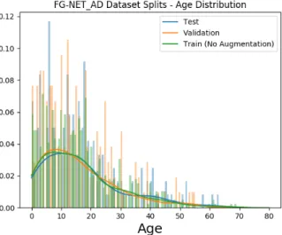
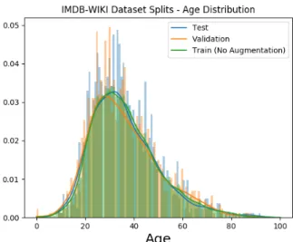
4.2 Age distribution on train/test/validation split of the FG-NET-AD dataset. . . 27
4.3 Age distribution on train/test/validation split of the MORPH2 dataset. . . 27
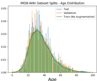
4.4 Age distribution on train/test/validation split of the IMDB-WIKI dataset. . . 28
4.5 Several Transformations of a MORPH2 image (before noise addition). . . 29
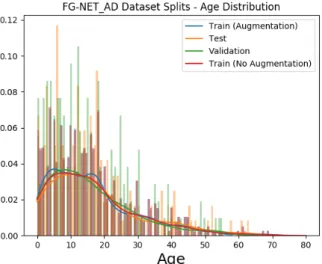
4.6 Age distribution on train/test/validation split of the FG-NET-AD dataset after data augmentation. . . 31
4.7 Age distribution on train/test/validation split of the MORPH2 dataset after data augmentation. . . 31
4.8 Age distribution on train/test/validation split of the IMDB-WIKI dataset after data augmentation. . . 32
4.9 Example of the 68 iBug Landmark notation [STZP13]. . . 33
4.10 Example of the transformation process. . . 35
4.11 Summary of Dataset Pipeline. . . 37
4.12 The architecture of the Baseline Model. Zero Padding is applied before each Con-volutional Layer. . . 38
4.13 The architecture of the Multi-View Rendering Model, inspired by [SMKL15]. . . 41
5.1 Examples of the best (first row) and worst (second row) prediction results of the Baseline model on the IMDB-WIKI dataset. . . 46
5.2 Examples of the best (first row) and worst (second row) prediction results of the Baseline model on the FG-NET-AD dataset. . . 48
5.3 Examples of the best (first row) and worst (second row) prediction results of the Baseline model on the MORPH2 dataset. . . 50
5.4 Confusion Matrices on IMDB-WIKI dataset. . . 52
5.5 Confusion Matrices on FG-NET-AD dataset. . . 53
5.6 Confusion Matrices on MORPH2 dataset. . . 54
A.1 The architecture of the Landmark Model. "..." indicate the rest of the model, as it is based on the baseline model. . . 67
A.2 The architecture of the U.V. Maps Model. "..." indicate the rest of the model, as it
is based on the baseline model. . . 68
A.3 The architecture of the 3DMM Model. "..." indicate the rest of the model, as it is based on the baseline model. . . 69
A.4 The architecture of the Point Cloud Model. "..." indicate the rest of the model, as it is based on the baseline model. . . 69
B.1 Confusion Matrices on IMDB-WIKI dataset (Pre-defined bags). . . 71
B.2 Confusion Matrices on FG-NET-AD dataset (Pre-defined bags). . . 72
3.1 Error in Mean Absolute Error (MAE) on datasets MORPH2 and FG-NET-AD. . . 17
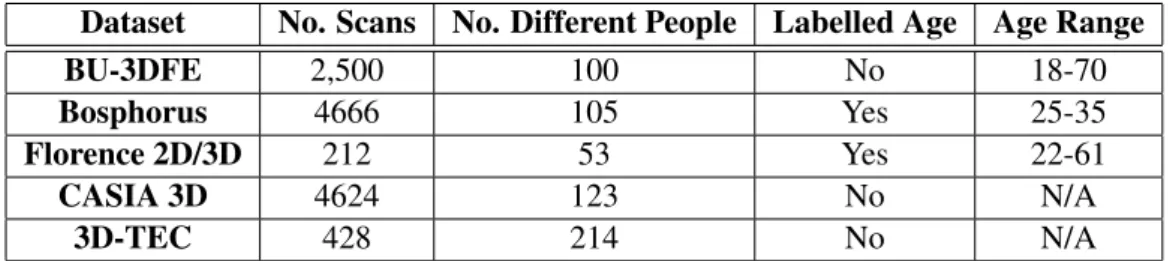
4.1 Detailed information on 3D Face Datasets. . . 30
5.1 MAE comparison of the models on IMDB-WIKI test set. . . 45
5.2 MAE comparison of the models on FG-NET-AD test set. . . 47
5.3 MAE comparison of the models on MORPH2 test set. . . 49
5.4 Cross Dataset Results for the Baseline model. . . 49
5.5 Cross Dataset Results for the Renderings model (Weighted Average Only). . . 50
5.6 Accuracy of each model for each age range on the IMDB-WIKI dataset. . . 52
5.7 Accuracy of each model for each age range on the FG-NET-AD dataset. . . 54
2D Two Dimensional Type
3D Three Dimensional
CNN Convolutional Neural Network SGD Stochastic Gradient Descent PCA Principal Component Analysis 3DMM 3D Morphable Model
MAE Mean Average Error ReLU Rectified Linear Unit
ADAM Adaptive Moment Estimation SVR Support Vector Regression AGES AGeing pattErn Subspace BIF Bio-Inspired Features LBP Local Binary Patterns LSTM Long-Short Term Memory LAP Looking at People
ICCV International Conference on Computer Vision ASM Active Shape Model
AOM Active Orientation Model LOO Leave One Out
Introduction
1.1
Motivation
The task of age estimation is a key component of an intelligent expert system, whose objective is to substitute the human component in many information systems from a variety of fields. Security focused tools can age restrict sensitive content from underaged users, whether this content is pur-chasable or viewable. Marketing tools steer personalized advertisement based on age information reducing the big overhead costs of advertising a product to the wrong target audience. Age infor-mation can be applied in many other sectors such as law enforcement, human-control interaction and social media.
Every human is equipped with the ability of estimating the age of someone with a simple face glance. It is similar to other biological trait detection tasks which humans are well versed on such as gender and ethnicity classification, health status diagnostic and facial expression interpre-tation, which are possible due to the existence of non-verbal characteristics. These innate human capabilities are essential every day tools and are an integral part of social interactions.
However, even humans can be easily fooled by other non-natural factors such as makeup, skin tan, both hair facial style, plastic surgery, among many others. Fashion changes dictate what kind of hairstyle young and old wear, hair dye products are cheap and easily obtainable and so is access to skin tanning products or even the beach. All these factors can influence someone’s perceived age and contribute to a more complex age estimation task.
Since current age estimation systems are appearance based, it is hard to tell if intelligent sys-tems also fall into the same pitfalls. The same problem occurs in face identification syssys-tems that must be robust to slight facial changes that may occur [SKP15]. The current state of the art on face identification has become sufficient for it to enter mainstream products. For example, we are currently seeing the market of mobile phones switching from fingerprint identification to face identification as the preferred method for unlocking a secure device, catching the public’s attention with the introduction of Apple’s IPhone X in 2017.
Although extensive research on facial age estimation, the use of the 3D shape of the face has been neglected from most studies. Scientists are aware that human facial skeleton changes
with age in particular the midface area, nose, eye sockets and jaw [MW12]. For this reason, we think it is important to take into consideration the facial structure, which contains 3D information, of a person when estimating one’s age, in addition to that person’s facial appearance which is commonly represented as a 2D image.
A lot of research age estimation through facial imaging has been done over the last years. Contests have been organized [EFP+15] in order to encourage researchers to delve into this field. Results took a huge leap in effectiveness with the introduction of deep learning, specially through the use of Convolutional Neural Networks (CNN).
1.2
Aim and Objectives
In this thesis, we will study how we can use 3D facial information to enhance age estimation from a single image. We aim to prove that improvements can be made on this research field by enhancing the existing state of the art approaches on 2D facial age estimation with the addition of 3D features representations.
The objectives of this thesis are:
• Study the current state of the art Deep Learning architectures, age estimation systems and techniques and 3D face modelling methods.
• Create a tool to collect, clean and pre-process the most commonly used age estimation publicly available datasets in a seamless way and fully personalized way.
• Create a CNN model which takes as input a single 2D image to serve as a baseline compar-ison for our future studies.
• Extend the collected 2D datasets with synthetically extracted 3D facial structure informa-tion, due to the lack of 3D facial datasets aimed at the age estimation task and incorporate these augmentations as part of the data processing pipeline previously mentioned.
• Extend the baseline model to take as additional inputs the extracted 3D facial information therefore creating multiple models with different architectures and input structures.
• Do a comparison study between the different models and different available 3D information to demonstrate the advantages and disadvantages of each when compared to the baseline. • Perform a cross-dataset evaluation of the models to determine how well these methods are
able to generalize to other data distributions.
• Understand the difficulties of this task by extending the error analysis to the prediction error distributions and accuracy metrics on age ranges.
Convolutional Neural Networks
2.1
Introduction
We can broadly categorize machine learning tasks into three types: Supervised Learning, Unsu-pervised Learning and Reinforcement Learning.
The first one, the most common form and the one that will be used throughout this thesis, is a task that consists on learning a function that maps a set of independent variables, i.e. the input, to a desired output, or a dependent variable. For this type of learning it is vital that we possess enough examples of input/output pairs on which the algorithm will train on. This paradigm’s key factor for a successful supervised learning algorithm is the algorithm’s ability to generalize to unseen data.
For many years, creating a machine-learning system required careful engineering and an ex-tensive expert knowledge to design an efficient feature extractor to transform raw data (such as characters of a text or pixels of an image) into a representation or abstraction, of which the under-lying system could learn patterns from.
Deep learning introduced representation learning with multiple levels of abstraction, obtained by composing simple but non-linear modules capable of transforming the data representation at one level into a representation level with a higher level of abstraction. When an image, for exam-ple, is fed into a deep learning algorithm, the learned features on the first representation layers will most likely represent the presence or absence of low level features such as edges, at certain loca-tion and direcloca-tion. Subsequent layers will detect combinaloca-tions of this edges that will in eventually create representations of textures and objects. By layering together enough transformations, it is possible to learn very complex functions. And by learning feature representation, features are no longer designed by humans and are learned directly from data [LBH15].
Convolutional Neural Networks were first introduced by [FM82] and later refined by [LHBB99], who first applied Back Propagation as the training algorithm. These models were inspired by neu-ral connections, hence the name, and are one of the most successful applications of the knowledge gathered by studying the brain. These models take advantage of structured data with spatially rel-evant information, whether it be audio (1D), images (2D) or volumetric images(3D) for example.
CNN’s were the basis of the Deep Learning boom when [KSH12] defeated its competitors on the ImageNet challenge by successfully applying a Deep CNN for the first time.
2.2
Convolutional Operator
A convolution operation (2.1), denoted with an asterisk∗, at momentt, is defined as a real valued operation between two functions, f and g, and it expresses how the shape of one function is modified by the other.
(f∗g)(t) = Z ∞
−∞
f(τ)g(t−τ)dτ (2.1)
The discrete valued convolution operator is given by Equation (2.2). This formulation of the same operation is necessary because the computational implementation of this operation requires it to support discrete values as input.
(f∗g)(t) =
∞
∑
−∞
f(τ)g(t−τ) (2.2)
Until now, our convolution formulations have supported kernels which support an infinite real set of values, i.e. g:R→R. When g has a finite support set, i.e. τ → {0,1, ...,M−1,M}, the convolution operation can be described with (2.3).
(f∗g)(t) = M
∑
τ=1
f(τ)g(t−τ) (2.3)
This is also important since in practice, our input and kernels are arrays of data with limited sizes. Moreover, these inputs and kernels can have multiple dimensions. The convolutional opera-tion can be rewritten to support this kind of multidimensional inputs. A 2D convoluopera-tion operaopera-tion is defined by: (f∗g)(i,j) = N
∑
γ=1 M∑
τ=1 f(τ,γ)g(i−τ,j−γ) (2.4)In practice, to avoid the unnecessary complexity of flipping the kernel or the input(convolutions are commutative), we use a very similar operation which is called cross-correlation (2.5), which does not flip neither the kernel or the input. This has no real impact on the operation in convolu-tional neural networks since the kernel is a set of features to be learned and it does not matter if the kernel is learned flipped or not as long as it is processed in the same manner every time.
(f∗g)(i,j) = N
∑
γ=1 M∑
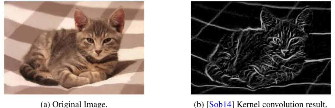
τ=1 f(i+τ,j+γ)g(τ,γ) (2.5) An image is the perfect example of a 2D input to a convolution operator as it defined by a grid of pixel values. Convolving the image with a kernel generates a feature map composed of kernel activated features at each block of the image.In Figure2.1, it is possible to see an example of the result of a convolution operation.
(a) Original Image. (b) [Sob14] Kernel convolution result. Figure 2.1: Example of the application of the Convolution Operation.
2.3
Convolutional Layer
Convolutional layers take advantage of the spatially relevant information of data with a grid-like topology, unlike Fully Connected layers which treats every element, which can be an element of the input or an element of a previous layer which we call a neuron, in the same manner. Each connection in a network contains a weighted parameter and each neuron a bias parameter. These parameters are very commonly referred to as theweightsof the network. Both of these types of parameters can be updated and are optimized during learning.
A Neural Network which contains Convolutional layers is typically called a Convolutional Neural Network (CNN), although they also usually possess other kind of layers such as Pooling and Fully Connected layers. A CNN is created by stacking these layers, which transform the input in a fully differentiable manner.
A Fully Connected Neural Network is composed by a series of Fully Connected layers. This network receives an 1D input which is iteratively transformed by the Fully Connected layers or hidden layers. "Hidden" comes from the fact that it represents the input as a result of an unknown function and from the fact that when looking at the interface of a network, only the input and output of the network are exposed. As mentioned before, each neuron of a Fully Connected layer is connected to every hidden neuron of the previous layer which creates a global receptive field. However, when dealing with multi dimensional data inputs it becomes unfeasible to connect every hidden neuron to all neurons in the previous layer.
On the other hand, Convolution Layers connect to a reduced local region, in space, of the input, resulting in a local receptive field with the size of the kernel, illustrated in Figure2.2. The Convolution Layer operation can be seen as a sliding window operation, where the kernelslides through the image across its width and height and computes the dot product between the kernel and the image at each location. From this operation results a 2D feature map which shows the activated kernel features at every location in the image. This sliding window operation can be performed multiple times in a single layer if multiple kernels are defined. The stride with which
Figure 2.2: Local Receptive Field example taken from [Nie15].
we slide and the number of kernels are hyperparameters that contribute to the shape of the output of a Convolutional Layer.
Since the same kernel is used to slide through the input, the weights of the connections are applied multiple times, therefore the elements of the output share kernel weights. This also form of parameter sharing introducestranslation equivariancemeaning that when the input is translated, the output is translated the same way [GBC16].
By choosing kernels smaller than the input in order to we are able to reduce the amount of connections. This occurs because while a Fully Connected contains(N+1)·Mnumber of learn-able parameters, whereNandMare the input and output sizes, in Convolutional Layers there are (N+1)·K, whereK=W·H·Dis the kernel size andW,HandDare the width, height and depth of the kernel.
The output of Convolutional Layer operation is described by Equation (2.6).
Oi,j,k= DI
∑
d=1 W∑
w=1 H∑
h=1 Ii+w,j+h,dWw,h,d,k+bw,h,d,k (2.6)2.4
Pooling Layer
Along with Convolutional Layers, Pooling layers are also an important component of a CNN. Usually, Pooling Layers are inserted after a stack of Convolutional Layers. The Pooling operation creates a smaller feature map by applying a filter to subregions of the input. The operation is then applied, much like the convolution operation, in a sliding window like fashion. An illustration of the operation can be seen in Figure2.3.
Pooling allows the network to become approximately invariant to small translations and at the same time, by reducing the resolution of the feature maps, it helps decrease the complexity of the network. In most applications of a CNN, translation invariance is a useful property since it is usually more important to know if a feature is present than to know precisely where it is. Using Pooling can be seen as adding an infinitely strong prior to the function the layer should learn, dictating it must be invariant to small translations [GBC16].
Figure 2.3: MaxPooling illustration example taken from [Kar18].
There are multiple ways to filter a region of features. Here we describe the two most common variations of a Pooling Operation:
• MaxPooling: MaxPooling finds the maximum value for each subregion and creates an out-put where each element is the maximum value of every region.
• AvgPooling: AvgPooling averages the feature values of each subregion and creates an out-put where each element is the average value of every region.
2.5
Activation
The Universal Approximation Theorem [Csá01] states that a neural network single hidden layer can approximate any continuous function on compact subsets of Rn., given enough hidden neurons and an activation function that is non-constant, bounded, and monotonically-increasing continu-ous, can approximate any continuous function on compact subsets ofRn.
Up until this point, the network would only apply a linear transformation to the input. More-over, the network would not satisfy the Universal Approximation Theorem therefore it wouldn’t be able to learn more complex linear functions. In order to do so, we must introduce non-linear activation functions. Activation functions are applied after a non-linear operation and are an element-wise operation which means it does not affect receptive fields.
Given an activation functionσ, the Equation (2.6) is rewritten as:
Oi,j,k= DI
∑
d=1 W∑
w=1 H∑
h=1 σ(Ii+w,j+h,dWw,h,d,k+bw,h,d,k) (2.7)The chosen functions need to be differentiable in order for the network to be trained. The most commonly used functions are:
• Sigmoid: The Sigmoid function, illustrated in Figure2.4a, is defined by: sigmoid(x) = 1
This biologically inspired function squashes the input values to a range of ]0,1[. How-ever, this function has two properties that pose major disadvantages which are the not zero-centered output and the fact it is more prone to gradient saturation.
• tanh: The Hyperbolic Tangent (tanh), illustrated in Figure2.4b, function is defined by: tanh(x) =e
2x−1
e2x+1 (2.9)
This function squashes the input value to the range ]−1,1[. Tanh is a rescaled sigmoid function however this version is zero-centered. Nonetheless, it still suffers from the gradient saturation problem.
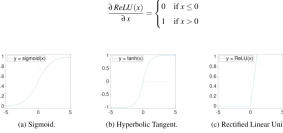
• ReLU [NH10]: The Rectified Linear Unit (ReLU), illustrated in Figure2.4c, function is defined by:
ReLU(x) =max(x,0) (2.10) Along with the reduction in computational complexity, ReLU fixes the gradient saturation issue present in the previous functions however it introduces other problems such as dead ReLU units. Subsequent iterations of ReLU such as LeakyReLU or Exponential Linear Units (ELU) address this issue. This function is not differentiable in all of its domain with its derivative atx=0 being undefined. In order to use back propagation, explained in Section 2.7, every operation in the network must be differentiable. In practice, the derivative of ReLU is defined as:
∂ReLU(x) ∂x = 0 ifx≤0 1 ifx>0 (2.11)
(a) Sigmoid. (b) Hyperbolic Tangent. (c) Rectified Linear Unit. Figure 2.4: Illustration of different activation functions.
2.6
Loss
As mentioned before, CNN’s usually contain Fully Connected Layers which are generally the last layers to be stacked. After high and low level feature extraction, we can take advantage of the global receptive field of these layers and perform a global transformation of the input.
The last layer is usually one dimensional with as many units as labels in the case of a classifi-cation problem or a single unit in case of a regression problem. The values of this last layer either represent the score, in the form of logits, of the input for each class or the estimated regressed value.
In order to train a CNN, we need to come up with an loss or cost function that can measure the quality of model’s predictions or regressions, given certain parameters. The network will be optimized in order to minimize this value. The most common loss function for classification problems is the Cross Entropy (2.12), applied after a Softmax (2.13) operation which squashes a vector of arbitrary values to a vector of real values, with each entry having a value in the range ]0,1]and∑Kk=1vk=1, while for regression problems is commonly used the Mean Squared Error (2.14) or the Absolute Squared Error (2.15) (MSE/MAE).
L(yˆ,y) =− N
∑
n=1 ynlog(yˆn) (2.12) σ(vk) = e zj ∑Nn=1evn (2.13) L(yˆ,y) = N∑
n=1 (yˆ−y)2 (2.14) L(yˆ,y) = N∑
n=0 |yˆ−y| (2.15)2.7
Back Propagation
For the network to output optimal values its parameters have to be adjusted. The optimization technique most commonly applied to CNN’s is gradient descent. In order to update the weights we need to compute the gradient of the loss w.r.t. the network’s parameters, which are the weights of the connections and bias. Due to the stacking nature of neural networks, the gradient of each layer can be propagated backwards to an earlier layer for a more efficient computation. This algorithm is named Back Propagation and is powered by the use of consecutive applications of the chain rule: δ(σ(x))0=∂ δ(σ(x)) ∂x = ∂ δ(σ(x)) ∂ σ(x) · ∂ σ(x) ∂x =δ 0 (σ(x))·σ0(x) (2.16)
The vanilla gradient descent algorithm is defined by Equation (2.17).
Wt+1=Wt−λ·∇L(Wt; ˆy,y) (2.17) whereWt indicates the model’s parameters on iterationt, in this case an epoch, andλ is a
weighting parameter called Learning Rate (LR), which dictates the size of the step taken in the direction of the negative gradient.
Up until this point, each parameter update was computed using the entire training dataset. When dealing with simple loss surfaces and small datasets this approach works however in practice we deal with extremely complex and non-convex, smooth loss surfaces and huge datasets in order to fight model overfitting which makes the task of fitting all the data in one iteration unfeasible. Instead, we can divide our training dataset into smaller chunks or batches and iteratively updating the networks parameters using each batch at a time which also takes advantage of adding more variance to the updates since the gradients are noisier. This optimization technique is called mini-batch gradient descent and can be defined by Equation (2.18). The size of the batch can vary and with batch size of one we call it Stochastic Gradient Descent (SGD), defined by Equation (2.19), whereWt now stands for the parameters on the batch iterationt.
Wt+1=Wt−λ·∇1 B B
∑
b=0 L(Wt; ˆyb,yb) (2.18) Wt+1=Wt−λ·∇L(Wt; ˆyi,yi) (2.19)Gradient descent can be further optimize by adding a hyper-parameter momentum,α , a
run-ning average of the gradients which helps reduce noisy variations in the direction of the gradient and enhances consistent ones. The update rules are defined as:
vt+1=αvt−λ·∇L(Wt; ˆy,y)
Wt+1=Wt+vt+1
(2.20)
Nesterov momentum [SMDH13] improves momentum by looking ahead and calculating the gradient using an approximate weights updated with the current momentum values. The Equation (2.20) can be updated as:
vt+1=αvt−λ·∇L(Wt+αvt; ˆy,y)
Wt+1=Wt+vt+1
(2.21)
Adagrad [DHS11] adapts the Learning Rate hyper-parameter to the model’s weights therefore removing the need to tweak the learning rate. It performs large updates for infrequent features and updates for frequent ones. This is done by taking into account the gradient at each update stept and modifying the Learning Rate w.r.t it, where each weight update rule is expressed by:
Wt+1,i=Wt,i−p λ Gt,ii+ε
·∇L(Wt,i; ˆyi,yi) (2.22)
whereGt,i ∈Rd,d is a diagonal matrix with each diagonal element representing the sum of the squares of the gradient w.r.tWi at update steptand with smoothing termε in order to avoid dividing by zero.
One of the most commonly used optimization techniques is Adaptive Moment Estimation (ADAM) [KB14]. ADAM keeps an exponential decaying average of previous Gt,i and of past gradients, similarly to momentum. This information is kept as:
gt =∇L(Wt; ˆy,y) vt+1=β1vt+ (1−β1)gt
st+1=β2st+ (1−β2)(gt)2
(2.23)
wheremtandstare estimates of the first and second central moment of the gradients, which are the expected value of the gradients and the variance, respectively. Sincemt andst are initialized with zeros, it is observed that the values are biased towards this value. Adam corrects this estimates by: ˆ mt= m t 1−β1 ˆ st= s t 1−β2 (2.24)
and then updates the weights with Equation (2.25). The hyper parametersβ1 andβ2 are the
exponential decay rates for the first and second moment of the gradients, respectively. [KB14] propose default values ofβ1=0.9 andβ2=0.999 which they empirically proved to work well in
practice. Wt+1=Wt−λ mˆ t+1 √ ˆ st+1+ε (2.25)
Literature Review
This Literature Review is divided in 2 sections. The first section is where a summary account of the research done on Age Estimation through 2D facial images is presented. This section is further divided into subtopics which include Appearance Base Feature Extraction and Deep Learning approaches. An additional subtopic on Apparent Age Estimation was added. Although Apparent Age Estimation is not the focus of this project, this research topic raised interesting ideas that might be applied to Biological or Real Age Estimation.
In the second section is available a brief overview of the work that has been done on 3D Face Modelling. This section is subsequently divided into two sections. In the first, the focus is on the study of Facial Landmark Detection while the latter is focused mainly on 3D Face Model Reconstruction.
3.1
Biological or Real Age Estimation
3.1.1 Appearance Base Feature ExtractionOne of the first approaches to facial age estimation was done by [HKL94]. In their work, they calculated six different ratios based on distances between facial landmarks. In addition to these ra-tios, they also implemented a very simple wrinkle detector. At the end, they were able to correctly classify each face from their 47 face image dataset as either baby, adult or senior.
In 2009, [LRBS09] used Active Appearance Model (AAM) [CET01] in conjunction with Sup-port Vector Machine Regression in order to tackle the FG-NET-AD [Lan04] dataset. Principal Component Analysis (PCA) [F.R01] was used to create a statistical model of the face that contains both shape variation and gray-level appearance features. First they modelled the shape variation by applying PCA to hand-annotated facial landmark data. Therefore any example can be annotated by:
where ¯xis the mean shape,Psa set of orthogonal principal components of the data andbsa set of parameters. The same is made for appearance features resulting in the following linear model:
g=g¯+Pgbg (3.2)
where ¯g is the mean shape, Pg a set of orthogonal principal components of the data andbg a set of parameters. The set of parameters bs and bg now define the model. They are further combined by adding a weighting factor and by applying PCA again to remove possible correlations between shape and appearance. To find a model that fits a 2D image, their model minimizes the difference between the original image and the recreated one. The way this is achieved is by learning the relationship between the reconstruction error and the error in the model parameters, therefore a model is trained iteratively to learn how to correct the model parameters according to the reconstruction error.
Figure 3.1: Example of an AAM reconstruction (left)/original (right) [CET01].
After the feature extraction process, these features are fed to an SVM [CV95] responsible for binarily classifying the image as an adult or a child. This outcome will be the deciding factor on whether the features are fed to a Support Vector Regression (SVR) model for adults or children. The chosen SVR will be responsible by outputting the final estimated age from a continuous range of age.
[GZSM07] proposed an Ageing Pattern Subspace(AGES) that defined a pattern as a sequence of a single person face images with different ages in temporal order. AGES can generate the miss-ing ages by applymiss-ing Expectation Maximization based algorithms. When creatmiss-ing a pattern, facial features are extracted using AMM [LRBS09]. The missing ages from the pattern are filled with the mean feature vector from all the individual’s facial features. Standard PCA is then applied to all patterns. Then they try to reconstruct the original images using the new pattern projection. The feature vector corresponding to the originally missing ages is updated by the new reconstructed feature vector. A new projection is then created from the new estimated features and the process repeats again until convergence ([GZSM07] provided proof of convergence). The age estimation for an unseen image is achieved by finding the ageing pattern most suitable for the image.
Still within the topic of feature extraction methods based on visual appearance, Local Binary Patterns (LBP) [Ots79] were used by [GN08] as image features since they can represent funda-mental properties of the image and its occurrence histogram is an effective texture feature for face descriptions. To perform age estimation on an new face image, spatial LBP histograms are produced and then used to classify the face as one of the six age classes, using a distance based classification method, either by using the distance between the new image’s LBP histogram and the mean histogram of each of the age classes or using a K-Nearest Neighbour Classifier [GN08]. Other techniques include using Gabor wavelet [GA09] and using Bio-Inspired Features (BIF), which [GMFH09] improved by using a pyramid of smaller Gabor filters with smaller sizes and problem-specific number of bands and orientations.
3.1.2 Deep Learning
With the increasingly good results Deep Learning techniques continue to provide on the Computer Vision research area, research applied to Real Age Estimation using these techniques has been the focus of a substantial amount of academic work [CZD+17,YLW+14,NZW+16,ZDH17,RTG15, HHM+17, QMB17] over the last years. CNN’s are the preferred technique when it comes to feature extraction for images in deep learning. One big advantage of Neural Networks is the ability to transfer their knowledge from one domain to another [OAE16,YCBL14]. Research shows that using pre-trained models on age estimation problems is advantageous [OAE16] whether we use a model trained on a broader classification problem such as the ImageNet dataset [DDS+09] or face specific classification challenge such as with the VGG-Face [PVZ15] model for face identification [QMB17].
[HHM+17] proposed an end-to-end deep embedding network for age estimation. To create a metric embedding we need to learn a function that can map an input to a feature space where the Euclidean distance (3.3) in this embedded space directly represent the semantic similarity of the inputs, and in this case, the features were learnt by triplet loss (3.4) using a CNN. These inputs can be anything from images [SKP15] to words [MCCD13]. They set out to create a multi-task classification problem in which they optimize their model using triplet loss in addiction to age estimation through discrete classification loss. With the addition of the triplet loss, the CNN can learn a metric space where the distance between similar ages is bigger than distant ages. Therefore, the features learnt by the network are more discriminative when it comes to performing the age estimation task.
D(Ia,Ib) =||f(Ia)−f(Ib)||22 (3.3)
The triplet loss gains it’s name by taking a triplet of inputs(Xta,X p
t ,Xtn)whereXtais the anchor of thetthtriplet,Xtpis the positive input with a similar semantic value as the anchor, in this case age, andXtnis the negative with a different semantic value. The triplet loss function is represented
by: L(Xta,X p t ,Xtn,WT) =max{0,m+D(Xta,X p t )−D(XtaXtn)} (3.4)
wheremis the margin parameter andWT are the weights of the feature extractor for which a CNN was used.
Still on the topic of multi-task classification, [NZW+16] use the age-related ordinal informa-tion and propose a multiple output CNN in order to perform age ordinal regression. They transform the ordinal regression into a series of binary classification sub-problems. These binary classifiers are responsible for predicting whether the rank of an image is above ark rank,k∈K, where K is the number of ranks, i.e. number of age ranges, which can be discrete or aggregated values. This technique was later improved by [CZD+17].
Other similar approaches were developed by [YLL15] and [TCT16], where the multi-task classification loss is formulated by adding the gender and gender specific age estimation losses. Multi-task learning can be seen as a form of inductive transfer which can help improve a model by introducing inductive bias. The inductive bias in the case of multi-task learning is produced by the sheer existence of multiple tasks, which causes the model to prefer the hypothesis that can solve more than one task. Multi-task learning usually leads to better generalization [Rud17].
More recently, a lot of focus on data augmentation using Generative Adversarial Networks [GPM+14] has been popping up in literature in many fields, such as autonomous driving [ASE17], medical imaging [FKA+18a] and also face identification [ZXKJ+17]. The idea of a GAN is to create a system where two networks are in constant competition in a zero-sum game. While one network tries to generate synthetic data indistinguishable from the original source data, the other is responsible for distinguishing generated data from original data. [FKA+18b] took this idea and applied it to the age estimation task. It took both FG-NET-AD and MORPH2 datasets and built a synthetic augmented instances of faces based on a simple trained GAN.
The current state of the art performance is hold by [ZLY+18] on both MORPH2 and FG-NET-AD datasets. They extract local facial characteristics from a cropped region estimated by a Long-Short Term Memory (LSTM) unit. They then combine their local extracted features with the global-image level features to perform their final estimation.
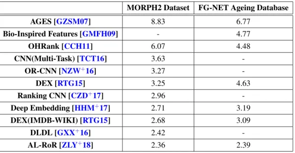
Table 3.1: Error in Mean Absolute Error (MAE) on datasets MORPH2 and FG-NET-AD.
MORPH2 Dataset FG-NET Ageing Database AGES [GZSM07] 8.83 6.77 Bio-Inspired Features [GMFH09] - 4.77 OHRank [CCH11] 6.07 4.48 CNN(Multi-Task) [TCT16] 3.63 -OR-CNN [NZW+16] 3.27 -DEX [RTG15] 3.25 4.63 Ranking CNN [CZD+17] 2.96 -Deep Embedding [HHM+17] 2.71 3.19 DEX(IMDB-WIKI) [RTG15] 2.68 3.09 DLDL [GXX+16] 2.42 -AL-RoR [ZLY+18] 2.36 2.39
A summary overview of the research done on age estimation using a single image utilizing the FG-NET-AD [Lan04] has been made available by [PLTC16]. It shows a consistent increase in interest on facial age estimation between 2005 and 2012.
3.1.3 Apparent Age Estimation From a Single Images
In 2015 and 2016, ChaLearn ran the Looking at People (LAP) apparent age estimation from a sin-gle face image challenges [EFP+15]. These challenges differ from traditional real age estimation in the sense that instead of focusing on trying to predict the biological age from images, it focuses on estimating age as it is perceived by other human beings. Along with the challenge proposal, ChaLearn made available the biggest datasets of apparent age annotated face images, the LAP datasets, one for each year of the competition.
In order to successfully tackle the 2015 challenge, [RTG15] from the Computer Vision Lab, ETH Zurich, proposed an ensemble of Convolution Neural Networks, using the VGG16 [SZ14] pretrained on the ImageNet dataset for image classification [RTG15], approaching the problem as multi-class classification problem and ended up winning the competition. They finetuned the ImageNet pretrained VGG16 network using their own collected dataset they called IMBD-WIKI. The dataset is publicly available at their website and contains 524,230 images. These images were then processed in order to obtain an aligned cropped image of the face by using an iterative rotation process without landmark detection. Afterwards, they divide the LAP dataset in 20 subsets, using each one to further finetune their IMDB-WIKI finetuned VGG16 network, therefore creating 20 different networks. When trained for classification, the output layer is composed of 101 softmax-normalized neurons, representing discrete ages from 0 to 100. They improve their predicted output
by computing a softmax expected value (3.5): E(O) = Y
∑
i=0 yioi (3.5)where O is a random variable with a Y number of finite outcomes, in this case 101, from 0 to 100,oi∈Oandyis the softmax output of the network for a given y. The final prediction is made by averaging every networks prediction.
In 2016, [MAE16] got fifth place by making very good use of an ensemble of VGG-Face [PVZ15] networks finetuned with the IMDB-WIKI dataset [RTG15]. Instead of representing every discrete age as a class, they use a softer age encoding and distributed the ages in groups of three to try and reduce the impact of the existing standard deviation of apparent age on the LAP dataset. After training and finetuning their models individual with a subset of augmented images from the LAP dataset, they pick the top 5 predicted classes of each model to do a weighted average which is then averaged for all 3 models to produce the final output.
[ABBD16], the winners of the 2015 LAP Challenge [EFP+15], noticed that the 2016 LAP dataset, in contrast to the 2015’s dataset, contained a considerable amount of face images of chil-dren in comparison with the previous dataset iteration. The standard deviation of the perceived age of children according to the dataset is inferior to the average over the whole dataset, which meant a bigger penalty would occur for each misclassification of a child’s apparent age. With this fact in mind, the authors created a 2-step approach using ensembles of VGG-Face [PVZ15] finetuned with the IMDB-WIKI dataset [RTG15]. The authors finetuned 11 networks separately with the competition dataset, using, instead of a discrete one hot encoding, a normalized label distribution according to the image face standard deviation, which they called the "general" prediction. Sep-arately, 3 VGG-Face [PVZ15] CNN’s were used as pretrained models to classify children’s age using a private dataset containing only children face images. These networks were trained using a one hot encoding. The two ensembles were then combined in such a way that if the "general" ensemble would classify an image as containing the face of a child, it would delegate further classification to the ensemble specialized in children.
3.2
Face Modelling
3.2.1 Facial Landmark Detection
An Active Shape Model (ASM) [CTCG95] is a model-based approach to modelling objects whose appearance is flexible. A deformable parametrized model shape is produced based on a training set and its parameters learn how the object’s shape can change. Therefore, it is able to fit new instances with similar shape. This involves an iterative procedure that requires following the new image’s gradient in order to fit a given model. [LTC97] applied this idea to facial shapes. This work allowed them to fit a face to a trained model using a 2D image. The resulting fitted model expresses the main facial keypoint locations as well as its shape. This approximation can then be used for gender classification, expression recognition, 3D face recovery, age estimation and
face alignment. AAM [CET01] extends this idea by combining the shape model with another parametrize model, the later representing the facial texture.
One of the first approaches to facial landmark detection making use of deep learning was developed by [SWT13]. The idea behind their work involved the use of a cascade of Convolutional Neural Networks. Distributed by 3 levels, the use of multiple stacked and parallel CNN allowed for a coarse-to-fine prediction, which involved feeding level 2 and 3 of the network with a cropped version of the original image around an initial facial landmark estimation, resulted in a more robust and accurate estimation of the points’ position. The project described by [SWT13] is able to regress the position of five facial landmarks.
Due to an increasing amount of lack of correspondence between datasets, in 2013 [STZP13] proposed a semi-automatic methodology as well as defining an academic standard for facial land-mark annotation, based on MultiPIE dataset annotation [GMC+08], with 68 well defined points of interest, the 68 iBug facial point annotations. Their tool allowed researchers to create a less error-prone way of annotating, that encourages cross-database experiments and have a substanti-ation amount of high quality landmark features. Building on top of the idea of AAM [LRBS09], [STZP13] created Active Orientation Models (AOM), proposing a model capable of outputting the 68 landmarks given a 2D image. They take an annotated subset of images with which they train an AOM. They then feed the AOM with a non-annotated subset. If the output is not manu-ally accepted as "good", another AOM is trained using both the original annotated subset and the "good" annotations of the previous AOM and another batch of synthetically produced annotations is created. When all images are accepted, the annotations on the non-annotated subset are manu-ally checked and corrected. This tool allowed them to produce annotated datasets with the same model from several previously non-annotated databases which they consider so accurate that they can be used as ground truth.
[BT17b] proposed a network which converts 2D landmarks annotations and converts them into 3D, allowing them to create the biggest 3D facial landmark dataset to date (of around 230 thousand images). They stacked 4 Hour-Glass networks [NYD16] on which they replace the Hour-Glass’s bottleneck residual block [HZRS15a] with [BT17a] version, which was shown to outperform [NYD16] when the same network parameters were used. They added to the common 3 channel input (RGB) 68 additional channels, each representing a 2D landmark with a 2D Gaussian distribution with a unit standard distribution around the landmark’s location. The network is able to then estimate the depth of 2D projections of the 3D landmark position using a Res-Net-152 [HZRS15a] network adapted to accept the image and the 2D projections as input and output the depth of each landmark.
3.2.2 3D Face Model Reconstruction
For many years, researchers have been trying to find a way to efficiently model a human face in three dimensions. One of the first to tackle this challenge was [Par74] in his PhD dissertation in 1974. He built a parametric model with each specific feature of the face being individually
designed and defined. By changing each face feature’s specific parameters he could generate different facial shapes and expressions.
In 1990, [BV99] proposed 3D Morphable Model (3DMM), the technique that would later become the most used approach to 3D facial shape reconstruction. They define a morphable face model as a 3D triangulated mesh built from a set of scanned faces. To create their model, they take each face from their set, and represent its geometry with a shape-vector which contains the 3 dimensional coordinates of each vertex of the mesh and a texture-vector, which in turn represent the RGB color values of each correspondent vertex in the shape-vector. By tweaking each element in the shape and texture vector, it is possible to generate new shapes and textures. Assuming all faces are in full correspondence, i.e., geometry vectors follow the same vertex order for every face, they fitted a multivariate normal distribution to their dataset containing 200 facial scans of young adults (100 female and 100 man), based on the averages of the shape and texture vectors. Then PCA [F.R01] is employed to construct a model with reduced number of parameters and these parameters are transformed into uncorrelated variables. They state they maintain 95% of the meshes variance by keeping the 100 principal components of each vector.
Arbitrarily, new face models can then be generated by varying the set of coefficients. However it is necessary to quantify the results in terms of their plausibility of being faces. The fitting of a new 2D face image to a 3DMM model is possible by first pre-aligning the face with the model and then updating the model parameters as well as rendering parameters by applying gradient descent optimization to the recreation error. The recreation error can be defined as the difference between the 2D image and the reconstruction of the image using the rendering of the face using the current 3DMM parameters as well as the rendering parameters. This method was then augmented to allow for extra parameterization of facial expressions [CWZ+14].
A combined use of the 3DMM [BV99] with 2D AAM [CET01] was shown to work by adding additional parameters to the AAM’s shape model in order for it to be able to represent 3D poses. Although they find that by constraining the AAM parametrization with a 3D shape model leads to an increase of the number of parameters up to a factor of 6, the new model possesses reduced flexibility which in turn leads to faster convergence.
A team at Imperial College London recently released their Large Scale Facial Model (LSFM) [BRZ+16]. This model is constructed out of more than nine thousand 3D facial scans. This allows for a better generalization of the face model in comparison with the 200 hundred facial scans, whose subjects have similar ethnicity and age, used by [BV99]. Due to their dataset’s diversity, they successfully created a collection of models tailored by gender, age and ethnicity. They also found a correlation between the 3DMM parameters and the age of the individual, reinforcing the statement that the 3D facial elements do contain pertinent age information.
Instead of fitting a 3DMM in an expensive iterative process that requires the rendering of the model at each iteration of the refinement process, [THMM16] designed a CNN capable of performing 3DMM parameter estimation directly from an input image. This allowed them to create a system with not only with a lower model reconstruction error but also a much faster 3DMM parameter estimation as a result of the rendering bypassing. Later on, they revamped their
model in order to adopt expression [CTH+18] parameters and more recently 3D reconstruction under extreme conditions, such as occlusions [THM+17].
[JBAT17] were able to bypass both the face alignment phase and 3DMM fitting by demon-strating that a single volumetric regression of the 3D face geometry is possible using only a 2D image. This reconstruction is made possible by developing an end-to-end architecture that uses two Hour-Glass network [NYD16] with skip connections and residual blocks [HZRS15a]. They also contribute by extending their architecture to a multi-task one where they fork their first HG into an HG responsible for regressing the 3D face structure and the second for extracting the 68 iBug facial landmarks [STZP13] in the from of a 2D Gaussian per channel corresponding to each landmark. [JBAT17] also added a guided network, instead of forking their tasks, because they argue that using facial landmarks can improve the network performance either during training or inference.
In early 2018, [FWS+18] proposed U.V. Position Map as the representation of a full 3D facial structure. Their U.V. coordinate system was created based on 3DMM [BV99], however the result-ing regressed model is not constrained by the original 3DMM model. The structure of the U.V. map can be seen in Figure3.2.
Figure 3.2: Structure of U.V. mapping [FWS+18].
This way, by directly regressing the position map from 2D images they can obtain both the 3D facial structure as well as the resulting face alignment. They train an encoder-decoder network to learn how to transfer the 2D RGB image into a regressed position map. In order for their model to learn its parameters, a weighted MAE (3.6) between the regressed position map and the ground truth position map is used, whereMis a weighting mask. The weighted component arises from the fact that MAE treats every point in the position map equally although some regions of the face contain more discriminative features. Therefore, their weight map helps enhance learning in regions corresponding to the centre of the face as well as the 68 iBug [STZP13] landmarks while neglecting the impact of regions such as the neck and body.
Loss(θ) =||P(x,y)−P(xˆ ,y)|| ·M(x,y) (3.6)
They outperform [BT17b] on the 3D landmark alignment task mainly due to the avoidance of using an extra network to estimate the depth position of the landmarks. As a result of this, it is also
able to reduce the runtime by more than 5 times when compared to [BT17b] as well as the model size, from 1.5GB to 160MB. [FWS+18] have made their code and pre-trained models available on Github, although they don’t share their training details.
Methodology
4.1
Datasets
In this section, we will explore some of the existing publicly available datasets for facial age estimation. We will investigate their origin, image quality, size and age range available. We will also evaluate their value in relation to each other, describing the weaknesses and strengths of each dataset.
4.1.1 IMDB-WIKI
The competition winners of the 2015 Looking at People International Conference on Computer Vision (ICCV) Challenge [EFP+15] scraped the internet, or more precisely, the Internet Movie Database (IMDB) website and Wikipedia’s biographical pages for images of faces with the its corresponding age information, creating the largest publicly available dataset of face images with age labelling, entitled the IMDB-WIKI dataset [RTG15].
Web Scrapping refers to accessing web pages, finding specified elements of that page, extract them and collect said extracted data in structured dataset [BW16]. In order to collect the image data with the correct age labelling, [RTG15], a team at ETH Zurich, extracted only the images which possessed timestamps (the date and time the picture was taken) in its metadata, a human face and the correspondent individual’s date of birth (as well as gender, which is not pertinent to this dissertation). They collected a total of 523,051 images, 460,723 and 62,328 from IMDB and Wikipedia respectively. Along with the dataset, they released a file containing all the meta information regarding the images such as: date of birth of the person in the image, data of image capture, gender, name, coordinate based location of the face in the image and face score. With this information, they were able to calculate the age of the person in the picture at the time of the picture’s capture and label the image accordingly.
The IMDB-WIKI dataset, although the largest available, does bears some a few cons. Since images are gathered by IMDB from many sources, images have a wide range of resolutions, fields of view and size ratios. Moreover, the dataset was not manually analysed, therefore any error from the web scrapping pipeline is not detected. This errors come in the form of wrong labelling,
wrong timestamps, mostly due to the nature of the images. Most images retrieved from the IMDB website are still frames captured from movies, which can have long production times making the timestamps and labelling incorrect.
The full dataset is available at the ETH Zurich Computer Vision Lab’s website, including cropped and raw versions, as well as pretrained VGG-16 Caffe models.
As mentioned in Section4.1.1, the IMDB-WIKI dataset is an extremely noisy dataset due to its content’s origin. The collected data contains low quality, non-human facial images such as sketches and animated figures, blank images, wrongly labelled images, among other issues. For this reason, [ZGG+17] spent a week manually removing non standard images. The resulting clean dataset was called IMDBWIKI-101 and possessed 440,607 out of the original 523,051, which means about 16% of the data was considered noisy. However, the team did not make their dataset available to the public, therefore we do not make use of this dataset.
Figure 4.1: Example of non-standard images on IMDB-WIKI dataset [ZGG+17].
4.1.2 MORPH2
The MORPH2 album release for Non-Commercial uses contains 55,000 unique face images of little over 13,000 individuals and it is the largest longitudinal face database. It is also the largest manually inspected dataset for age estimation studies. The images were taken in a controlled environment from 2003 to late 2007. The ages present on the dataset range from 16 to 77. The average number of pictures per individual is 4 with an average of 164 days between each picture. More details are available in theMORPH Non-Commercial Release Whitepaper. Each image of the dataset has a resolution of either 200x240 or 400x480, maintaining the image ration whatever the resolution.
The MORPH Database for academic use was available for free until 2017 and now costs 199.00$ US dollars. However, we directly contacted Dr. Karl Ricanek Jr., director of the Face Ageing Group, who was able to provide us with the dataset for free. We would like to thank Dr. Karl Ricanek Jr. for his generosity and support. The dataset is now available at theFace Ageing Group’s website.
4.1.3 FG-NET Ageing Database
The FG-NET Ageing Database, or FG-NET-AD, was created in 2004 by the Face & Gesture Recognition Working Group, a multi institution initiative funded by the European Union. The aim of the project was to encourage research and the development of technologies in the area of face recognition and age estimation [Lan04].
This dataset contains 1002 face images of 82 different people, with their ages ranging between 0 to 69 years. The dataset is organized to present images of the same person in several stages of their lives. The pictures were not taken in a controlled environment and some, specially in the range from 0-10, are grayscaled. The dataset does not have a fixed image resolution. In addition to this, the images also contain a wide range of resolutions, image sharpnesses, scene illuminations, 3D poses and facial expressions. [PLTFC15] gives a more detailed overview of the dataset, including an overview of the research done in several areas with a reliance on the FG-NET-AD dataset.
The original website supporting the free release of the FG-NET-AD dataset is not online at the time of writing this thesis. Alternative mirrors are available elsewhere. We downloaded our dataset fromYanwei Fu’s personal website.
4.2
Data Pre-Processing
In this section, we will summarize the dataset pre-processing pipeline of our implementation. Each datasets goes through an iterative transformation process before all the data is extracted from said dataset.
4.2.1 Dataset Oriented Pre-Processing
Each dataset has particular characteristics that force us to approach its processing in a different way. This might be because of file format, labelling technique, folder organization, image charac-teristics (resolution, aspect ratio, colour encoding), among others. Below we will go over aspects of data pre processing required for each dataset.
The creators of the IMDB-WIKI used an iterative process of rotating the image, running the off-the-shelf face detector of [MBPVG14] and picking the detection with highest detection score. Afterwards, they rotate their cropping with a 40% margin in order to obtain an up-frontal position [RTG15]. They state that in their initial observations, this method works better than landmark detection then alignment and for this reason they adopt this strategy.
In this thesis, we use their publicly released cropped images. These images are cropped using the strategy previously described. However, we make use of the available provided image metadata and only use images that obtained a face score of 1.0, the maximum value. Moreover, we discard any image where a second person is detected (which increases the risk of wrong age labelling) as well as any image with a labelled age above 100 years old. The reason we are imposing very strict rules, is because we want to be assured high quality images even though there is no previous human
validation. After all this processing, we are left with over 100 thousand images which makes it a too large of a dataset to perform the next steps in a reasonable time with the resources we have. For this reason, we randomly sample 30 thousand images from the high quality set. We should point out that even after such a severe sampling, the subset is still larger than the FG-NET-AD and MORPH2 datasets.
After this initial processing, IMDB-WIKI images follows the same process as FG-NET-AD and MORPH2. Both datasets have their images already cropped around the face of the person since the images were manually inspected. Therefore, it is safe to assume that every image in these datasets have a single face present in the image.
Although the age labelling on the FG-NET-AD and MORPH2 datasets is contained within each image filename they do not employ the same format. Therefore, we relabel the images by the standard of having the last 3 characters before the file format be the person’s age, from "000" to "100".
Be that as it may, we want our results to be comparable to the available literature benchmarks therefore we must adhere by some previously set standards. In 2011, [CCH11] manually selected 5,492 images of people of Caucasian descent, out of the 55,608 available images on the MORPH2 dataset. The reason behind this selection was to reduce the variation between different ethnic groups present in the dataset. Since then, most literature follows this setup [RTG15,HHM+17, NZW+16,WGK15,ZLY+18] and to be able to perform a fair comparison we also adopt this setup.
4.2.2 Training/Validation/Testing Dataset Splitting
To validate the results of our models and ensure the models are capable of generalize to previously unseen data we need to split the model in a training and testing set. We also create subset of the training set to be used as a validation. Validation data will be used to estimate how well our model is generalizing and performing reductions to the algorithm’s learning rate or perform Early Stopping if the model either ends up overfitting the training data or we fail to see significant improvements each epoch.
Even though we wish for our results to be comparable to literature, we will not follow the stan-dard validation process for the FG-NET-AD dataset. Over the years, researchers would use Leave One Out(LOO) cross-validation to validate their results on this dataset. This implies creating more than 82 identical models, one for each person, and trained them with the dataset while leaving one person out and each person being left out once. This is not feasible in the scope of this thesis due to complexity of the models used, time constraints and available computational resources. Instead, we will employ the same validation strategy we use for MORPH2 and IMDB-WIKI.
We follow a 60/20/20 percentage split methodology on our training, validation and test sets. Although there is no standard when it comes to the splitting percentage, our approach has been previously used in literature [RTG15,HHM+17,GXX+16] and proven to give good results. More importantly, each set should accurately represent the overall data distribution of the dataset. We randomly split the original dataset, we should expect every split to follow the same distribution.
We confirm this to be the case in Figure4.2,4.3 and4.4 with the FG-NET-AD, MORPH2 and IMDB-WIKI age distributions histograms.
Figure 4.2: Age distribution on train/test/validation split of the FG-NET-AD dataset.
Figure 4.3: Age distribution on train/test/validation split of the MORPH2 dataset.
4.2.3 Data Augmentation
Deep learning techniques are very prone to overfit if fed with a small amount of data, i.e. the models end up memorizing the training data, becoming incapable of generalizing to new unseen data. One of the deciding factors for the success of the AlexNet [KSH12] model in 2012 was the fact they used extensive data augmentation techniques on the existing ImageNet dataset. By using a combination of cropping and flipping techniques they were able to augment their dataset by a factor of 2048. Without it their model suffered from "substantial overfitting" and they would
Figure 4.4: Age distribution on train/test/validation split of the IMDB-WIKI dataset.
have been forced to use a smaller model. With this fact in mind, we will employ data augmenta-tion techniques on the used datasets, except on IMDB-WIKI. This decision is due to the fact that IMDB-WIKI is large enough to be used without any augmentation. Moreover, the results compar-isons with state of the art approaches will not include IMDB-WIKI because no information about the performance of age estimation models has ever been reported on this dataset. Therefore there is no need to extensively test the performance of the models on this dataset. These factors, coupled with limited computational power availability, support this decision.
Different types of data augmentation in the image field are available. We are now going to summarize some of the possible image transformations:
• Flipping: Flipping images creates a mirror image of the original image. The flipping axis can either be horizontal or vertical. It is computationally efficient since it only requires to invert either rows or columns of the image. In our implementation we only perform a horizontal flip [RTG15,KSH12,BT17b]. Vertical flipping is not useful within this context since faces are usually captured in an upwards position and making the model robust to this kind of data would be inconsequential.
• Cropping: Cropping relies on sampling a sub-region of the original image. In our imple-mentation we perform 10 random crops of a region 80% smaller of our original image and its horizontally flipped version. [RTG15,KSH12]
• Rotation: Applying a rotation to an image might results in it having different bounds. This means the image will then have to be rectified. In our implementation, we rotate our pre-processed images by -15 and 15 degrees. We then rectify our rotated images by fitting, through downscaling, the rotated image in the same input space as the original image and zero pad the remaining space, which means the original image will be scaled down in addi-tion to being rotated.[RTG15,KSH12,BT17b]
![Figure 3.2: Structure of U.V. mapping [FWS + 18].](https://thumb-us.123doks.com/thumbv2/123dok_us/1284358.2672467/39.892.217.724.559.746/figure-structure-u-v-mapping-fws.webp)
![Figure 4.1: Example of non-standard images on IMDB-WIKI dataset [ZGG + 17].](https://thumb-us.123doks.com/thumbv2/123dok_us/1284358.2672467/42.892.236.619.463.676/figure-example-standard-images-imdb-wiki-dataset-zgg.webp)