Air Force Institute of Technology
AFIT Scholar
Theses and Dissertations Student Graduate Works
12-26-2014
Improving Non-Linear Approaches to Anomaly
Detection, Class Separation, and Visualization
Todd J. Paciencia
Follow this and additional works at:https://scholar.afit.edu/etd
Part of theOperational Research Commons
Recommended Citation
Paciencia, Todd J., "Improving Non-Linear Approaches to Anomaly Detection, Class Separation, and Visualization" (2014).Theses and Dissertations. 10.
IMPROVING NON-LINEAR APPROACHES TO ANOMALY DETECTION, CLASS SEPARATION, AND VISUALIZATION
DISSERTATION
Todd J. Paciencia, Major, USAF AFIT-ENS-DS-14-D-15
DEPARTMENT OF THE AIR FORCE AIR UNIVERSITY
AIR FORCE INSTITUTE OF TECHNOLOGY
Wright-Patterson Air Force Base, Ohio
DISTRIBUTION STATEMENT A:
The views expressed in this dissertation are those of the author and do not reflect the official policy or position of the United States Air Force, the Department of Defense, or the United States Government.
This material is declared a work of the U.S. Government and is not subject to copyright protection in the United States.
AFIT-ENS-DS-14-D-15
IMPROVING NON-LINEAR APPROACHES TO ANOMALY DETECTION, CLASS SEPARATION, AND VISUALIZATION
DISSERTATION
Presented to the Faculty
Graduate School of Engineering and Management Air Force Institute of Technology
Air University
Air Education and Training Command in Partial Fulfillment of the Requirements for the Degree of Doctor of Philosophy in Operations Research
Todd J. Paciencia, B.A., M.S. Major, USAF
December 2014
DISTRIBUTION STATEMENT A:
AFIT-ENS-DS-14-D-15
IMPROVING NON-LINEAR APPROACHES TO ANOMALY DETECTION, CLASS SEPARATION, AND VISUALIZATION
Todd J. Paciencia, B.A., M.S. Major, USAF
Approved:
/signed/
Kenneth W. Bauer Jr., Ph.D. (Chairman) /signed/
James W. Chrissis, Ph.D. (Member)
/signed/ Mark E. Oxley, Ph.D. (Member)
4 Dec 2014 Date 4 Dec 2014 Date 4 Dec 2014 Date Accepted:
AFIT-ENS-DS-14-D-15
Abstract
Linear approaches for multivariate data are popular due to their lower complexity, reduced computational time, and easier interpretation. In many cases, linear approaches produce adequate results; however, non-linear methods may generate more robust transformations, features, and decision boundaries. Of course, these non-linear methods present their own unique challenges that often inhibit their use.
In this research, improvements to existing non-linear techniques are investigated for the purposes of providing better, timely class separation and improved anomaly detection on various multivariate datasets, culminating in application to anomaly detection in hyperspectral imagery. Primarily, kernel-based methods are investigated, with some consideration towards other methods. Improvements to existing linear-based algorithms are also explored. Here, it is assumed that any classes in the data have minimal overlap in the originating space or can be made to have minimal overlap in a transformed space, and that class information is unknowna priori. Further, improvements are demonstrated for global anomaly detection on a variety of hyperspectral imagery, utilizing fusion of spatial and spectral information, factor analysis, clustering, and screening. Additionally, new approaches forn-dimensional visualization of data and decision boundaries are developed.
Acknowledgments
I would like to thank my family and friends, for their constant support as I engaged in a battle of wills with this endeavor and myself. I would also like to thank my committee members for supporting me with assistance and patience, and enabling me to complete this in my own unique and likely bizarre way.
My biggest thanks extends to Dr. Bauer, for keeping me positive, allowing me to chase many a rabbit down holes as I insisted on doing, and for the often timely insights. I generated many ”hydra” despite knowing not to do so, and it admittedly took me some time to understand that simpler methods can be just as powerful as their complex, extravagant counterparts. I hope that this final result is something that you can be proud of.
A final thanks to Trevor. Both for worldly insights..., and for having patience the many times I asked you a random question about an old dataset or algorithm as if you had generated them.
Table of Contents Page Abstract . . . iv Acknowledgments . . . v Table of Contents . . . vi List of Figures . . . x
List of Tables . . . xvii
I. Introduction . . . 1
1.1 Problem Definition and Background . . . 1
1.2 Assumptions . . . 3
1.3 Research Objectives . . . 4
1.3.1 Purposeful Visualization of High-Dimensional Data . . . 5
1.3.2 Improved Class Separation . . . 5
1.3.3 Improvements to Global Anomaly Detection in Hyperspectral Imagery . . . 6
1.4 Dissertation Outline . . . 6
II. Overview of Data Sets . . . 8
2.1 Data Imputation . . . 8
2.2 Multivariate . . . 9
2.2.1 Breast Cancer Wisconsin (Diagnostic) . . . 9
2.2.2 Chainlink . . . 10 2.2.3 Modified Banana . . . 10 2.2.4 Half-Moons . . . 10 2.2.5 Fisher Iris . . . 10 2.2.6 Pima . . . 11 2.2.7 Vertebral Column . . . 12 2.2.8 Hepta . . . 12 2.2.9 Wine . . . 12 2.2.10 Wine Quality . . . 13 2.2.11 MNIST . . . 13 2.2.12 Arcene . . . 13 2.3 Hyperspectral Imagery . . . 15
Page
2.3.1 Special Considerations for HSI . . . 15
2.3.1.1 Atmospheric Properties . . . 16 2.3.1.2 Scaling . . . 18 2.3.1.3 Correlation . . . 18 2.3.1.4 Truth Masks . . . 21 2.3.2 HYDICE-Derived . . . 22 2.3.3 AVIRIS . . . 25 2.3.4 Pavia . . . 26 2.3.5 SpecTIR . . . 28 2.3.6 HyMap . . . 32
III. General Methods . . . 34
3.1 General Dimension Reduction Techniques . . . 34
3.2 Principal Component Analysis . . . 36
3.3 Kernel Principal Component Analysis . . . 37
3.4 Factor Analysis . . . 41
3.5 Locally Linear Embedding . . . 44
3.6 Discriminant Analysis . . . 50
3.7 Wavelets . . . 53
3.7.1 Shrinking/Smoothing . . . 57
3.7.2 Application of Wavelets to HSI . . . 58
3.8 k-Nearest Neighbors . . . 60
3.9 Clustering . . . 61
3.9.1 k-Means . . . 61
3.9.2 X-means . . . 65
3.9.3 Affinity Propagation . . . 67
3.9.4 Spectral Clustering . . . 69
3.10 Independent Component Analysis . . . 69
3.11 Anomaly Detection in Hyperspectral Imagery . . . 71
3.11.1 RX-Based and Uniform Detectors . . . 72
3.11.1.1 RX-Based Detectors . . . 73
3.11.1.2 Low-Probability Detection Method . . . 76
3.11.1.3 Kernel RX . . . 77
3.11.1.4 General Likelihood Ratio Test . . . 78
3.11.1.5 Windows . . . 80
3.11.1.6 Iterative RX . . . 82
3.11.1.7 Linear RX . . . 83
3.11.2 Topology Anomaly Detector . . . 83
Page
3.11.6 Means of Identifying, Thresholding, and Comparing Anomalies . . 92
3.11.6.1 Thresholding . . . 92
3.11.6.2 Semi-Parametric Test . . . 93
3.11.6.3 Non-Parametric F-Distribution Test . . . 96
3.11.6.4 Spectral Angle Mapper . . . 97
3.11.6.5 Spectral Information Divergence . . . 97
3.12 Image Complexity . . . 98
3.13 Receiver Operating Curves . . . 100
IV. Investigating Hyperspectral Bands and Truth Masks . . . 103
4.1 Similarity Metrics . . . 103
4.2 Similarity/Dissimilarity Plots . . . 109
4.3 Analysis of Truth Masks and Border Pixels . . . 114
4.3.1 HYDICE . . . 114
4.3.2 HyMAP . . . 121
4.3.3 AVIRIS & Pavia . . . 122
4.4 Additional ROC Metrics . . . 123
4.5 Hyperspectral Band Selection and Analysis . . . 125
4.5.1 Band Selection Method and HYDICE-Derived Data . . . 133
4.5.2 AVIRIS . . . 143 4.5.3 Pavia . . . 147 4.5.4 SpecTIR . . . 149 4.5.5 HyMap . . . 153 4.5.6 Arcene . . . 154 V. n-Dimensional Visualization . . . 161 5.1 Literature Review . . . 161
5.2 Dimensionality Reduction and Random Projections . . . 165
5.3 Hyper-Radial Visualization and Improvements . . . 169
5.3.1 Determining Optimal Groupings . . . 174
5.3.2 3-Dimensional Hyper-Radial Visualization . . . 183
5.3.3 Further Visualization Analysis . . . 186
VI. Factor-Based Global Anomaly Detection . . . 192
6.1 Existing Component-Based Global Anomaly Detection . . . 193
6.2 Component Generation and Selection . . . 197
6.3 Direct Application of Factor Analysis . . . 204
6.4 Investigating Specifics of the Framework . . . 211
Page
VII. Large-Scale Kernel Principal Component Analysis . . . 244
7.1 Literature Review . . . 244
7.1.1 Eigen-Decomposition . . . 244
7.1.2 Landmark Points . . . 247
7.1.3 Optimal Kernels . . . 249
7.1.4 Further Algorithmic Considerations . . . 251
7.1.5 Choosing Discriminating Components . . . 252
7.2 Approximate Kernel Factor Analysis . . . 255
7.3 Skeleton Generation . . . 256
7.3.1 Development of Large-Scale Skeleton Approaches . . . 257
7.3.2 Skeleton Analysis . . . 259
7.3.3 Resulting KPCs Analysis . . . 267
7.4 KIGFAAD . . . 277
VIII.Support Vector Data Description . . . 289
8.1 Literature Review . . . 289
8.1.1 SVDD for Anomaly Detection . . . 289
8.1.2 Training Set and Spread Parameter Considerations . . . 293
8.1.3 SemiBoost . . . 295
8.2 Unsupervised Training Set Generation and Parameter Optimization . . . 296
8.3 Unsupervised SVDD (USVDD) . . . 300
IX. Summary of Contributions . . . 310
9.1 Review . . . 310
9.2 Insights . . . 312
9.3 Potential Future Research . . . 313
9.3.1 HSI Band Selection Refinement . . . 313
9.3.2 GFAAD Refinement . . . 313
9.3.3 Finding Better Unsupervised Boundaries for SVDD . . . 314
9.3.4 Improving Non-Linear Anomaly Detection . . . 314
9.4 Conclusion . . . 315
Bibliography . . . 316
List of Figures
Figure Page
1.1 HSI Image Radiance Example. . . 2
2.1 2-Class Geometric Problems. . . 11
2.2 Hepta dataset. . . 12
2.3 Example MNIST Digit: 5. . . 14
2.4 Arcene Class Mean Vectors. . . 15
2.5 Spectral Region Locations [81]. . . 16
2.6 ARES1D Covariance Eigenvalues Comparison. . . 19
2.7 ARES1D Window Correlation. . . 20
2.8 AVIRIS Deepwater Scene1 Sample. . . 20
2.9 ARES1D Band Correlation. . . 21
2.10 Natural No-Target HYDICE Images. . . 22
2.11 Three HYDICE Images and Number of Targets. . . 23
2.12 Three HYDICE Images and Number of Targets. . . 24
2.13 HYDICE run03m20. . . 25
2.14 AVIRIS Images. . . 27
2.15 Pavia Centre Scene. . . 30
2.16 Pavia University Scene. . . 30
2.17 Pavia University Bands. . . 31
2.18 SpecTIR Images [6]. . . 31
2.19 Cooke City, MT Image. . . 33
3.1 Loadings Comparison. . . 44
3.2 Factor Score Comparisons. . . 45
Figure Page
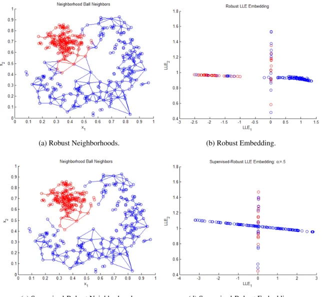
3.4 Banana Dataset RLLE and Supervised RLLE Example. . . 51
3.5 DWT Decomposition [162]. . . 56
3.6 Workflow Diagrams for PCA and PCA Involving Wavelets [87]. . . 59
3.7 KD Tree Example [12]. . . 61
3.8 Refined K-Means Comparison: Hepta. . . 63
3.9 Clustering Applied to Pavia University. . . 65
3.10 Clustering Applied to ARES1D. . . 66
3.11 RX-Like Detectors. . . 71
3.12 Distance Comparison on Two Data Sets. . . 74
3.13 Dual Cocentric Window [133]. . . 81
3.14 Window vs. Line. . . 84
3.15 AutoGAD. . . 85
3.16 Pixel×Band Representation. . . 86
3.17 Finding the Eigenvalue Cutoff[111]. . . 86
3.18 MPCA Overview [107]. . . 90
3.19 (a)Plot of gray values from RXD. (b) Histogram of (a). (c) Enlargement of right tail in (b) [46]. . . 93
3.20 Zero-Bin Detection [107]. . . 94
3.21 Comparison of Samples for Anomaly Detection [180]. . . 95
3.22 Truth and Prediction Example: Targets White. . . 102
4.1 Distance Comparisons. . . 104
4.2 PDF Metric Comparisons. . . 106
4.3 Metric Type Comparisons. . . 107
Figure Page
4.6 Example of Similarity/Dissimilarity Plot [15]. . . 110
4.7 Fisher Iris Similarity-Dissimilarity Plot. . . 111
4.8 Breast Cancer Similarity-Dissimilarity Plots. . . 113
4.9 Similarity-Dissimilarity Plot - SAM,k=5: ARES4F. . . 113
4.10 Similarity-Dissimilarity Plot -L2,k= 5: ARES4F. . . 114
4.11 ARES3F Similarity-Dissimilarity Plots. . . 117
4.12 ARES3F Plot: Target and Border vs. Background. . . 118
4.13 ARES1D Similarity-Dissimilarity Plots. . . 119
4.14 Border Pixel Dissimilarities withk= 5. . . 120
4.15 HyMAP Truth Mask Analysis. . . 122
4.16 AVIRIS Similarity-Dissimilarity: k= 5. . . 124
4.17 Pavia Univ Similarity/Dissimilarity Ratio: k= 5. . . 126
4.18 Band Selection Methodology [136]. . . 128
4.19 Band-by-Band Correlation Magnitude. . . 133
4.20 Simplistic Band Selection. . . 135
4.21 HYDICE Band Metrics. . . 136
4.22 HYDICE: max i,j Bi,j,p. . . 137
4.23 Specific Variance: ARES Images. . . 138
4.24 Specific Variance: MDSL Effect. . . 139
4.25 Band Selection Methodology. . . 140
4.26 HYDICE Images: Threshold Sensitivity. . . 141
4.27 HYDICE Threshold Sensitivities. . . 142
4.28 HYDICE Band Examples: Radiance Values. . . 143
4.29 AVIRIS Pixel Signatures Sample. . . 145
Figure Page
4.31 AVIRIS Threshold Sensitivities. . . 146
4.32 AVIRIS Specific Variance Sensitivities. . . 147
4.33 VirginIslands1 Band Comparison. . . 148
4.34 ROSIS Images: Threshold Sensitivity. . . 149
4.35 SpecTIR Images’ max i,j Bi,j,p. . . 150
4.36 SpecTIR: Threshold Sensitivity. . . 150
4.37 SpecTIR: Specific Variance Threshold. . . 151
4.38 RedSea Band Comparison. . . 152
4.39 HyMAP Bands. . . 153
4.40 HyMAP Band 63. . . 154
4.41 Number of Bands Removed By Threshold. . . 155
4.42 Arcene Feature Metrics. . . 156
4.43 Number of Features Removed: Original Process. . . 157
4.44 Number of Features Removed: Modified Process. . . 158
4.45 Feature Examples. . . 159
5.1 Parallel Coordinates Example. . . 162
5.2 Anchor-Based Visualizations [82]. . . 164
5.3 Hyperspace Diagonal Counting [11, 169]. . . 165
5.4 k0Values as a Function of,q, andN. . . 168
5.5 HRV: Fisher Iris. . . 172
5.6 HRV Radial [164]. . . 172
5.7 HRV Using Mahalanobis Distance. . . 173
5.8 Vertebral Column J1. . . 177
Figure Page
5.11 Breast CancerσComparison. . . 180
5.12 Wine Quality. . . 181 5.13 Wine J1. . . 185 5.14 Wine Visualizations. . . 185 5.15 MNIST. . . 186 5.16 MNISTJ1. . . 187 5.17 ARES1D Visualization. . . 188
5.18 ARES1D and ARES2D Comparison. . . 189
6.1 ARES1D Factors. . . 199
6.2 ARES4F Factors. . . 200
6.3 ARES4F PCs. . . 201
6.4 ARES1F ICs. . . 202
6.5 ARES1F Factor. . . 203
6.6 Training Set Max Scores and PA SNRs. . . 212
6.7 Other Images’ Max Scores and PA SNRs. . . 213
6.8 Training PA SNRs AfterIinit =3. . . 213
6.9 Experiment 3 Rates. . . 216
6.10 Experiment 4 Rates. . . 219
6.11 Zero-Bin Considerations. . . 220
6.12 Potential Anomalies. . . 221
6.13 Comparison With/Without Sensor Error. . . 223
6.14 General GFAAD Process. . . 224
6.15 IGFAAD. . . 230
6.16 run03m20 Anomaly Declarations. . . 238
Figure Page
6.18 ARES2D Anomaly Declarations. . . 240
6.19 Scene1 Anomaly Declarations. . . 240
6.20 IGFAAD Anomaly Declarations. . . 242
6.21 ROC Comparisons. . . 243
7.1 Optimal Kernel Example. . . 251
7.2 LAP and PLAP Half-Moon Example. . . 260
7.3 Center Comparisons. . . 261
7.4 Half-Moons Comparison. . . 262
7.5 Chain Links Landmark Version Comparison. . . 263
7.6 ARES1D LAP withm= 1000. . . 264
7.7 VirginIslands1 LAP Centers. . . 264
7.8 VirginIslands1 LAP Center Comparisons. . . 265
7.9 Maximin Landmarks &k-means Assignments. . . 268
7.10 Pima Eigenvectors and Values. . . 269
7.11 Pima Eigenvectors and Values. . . 270
7.12 ARES1D KFA Scores. . . 271
7.13 ARES1D KFA Scores: σ= √20. . . 272
7.14 ARES1F Scores. . . 273
7.15 ARES1Dk-Means Skeleton Comparisons. . . 275
7.16 ARES1Fk-means and NyAppox (NA) Skeleton Comparisons. . . 276
7.17 LLE Scores. . . 278
7.18 KIGFAAD Process. . . 279
7.19 KRX ROCs vs. Initial KIGFAAD Operating Points. . . 280
Figure Page
8.2 BACON Double-Screening Approach. . . 298
8.3 BACON Double Screening Results. . . 300
8.4 Landmark Generation for Optimal Kernel. . . 301
8.5 Kernel Selection: ARES2D. . . 303
8.6 SVDD Comparison: Forest Scenes. . . 305
8.7 SVDD Comparison: Desert and Water. . . 306
8.8 SemiBoost USVDD. . . 307
8.9 Fused IFGAAD and USVDD Results. . . 308
List of Tables
Table Page
2.1 HYDICE Image Properties. . . 26
2.2 AVIRIS Image Properties. . . 27
2.3 Pavia Sets Truth Data. . . 29
3.1 Dimension Reduction Technique Properties [149]. . . 35
4.1 Breast Cancer PAS. . . 112
4.2 Pima PAS’. . . 112
4.3 HYDICE ARES Fisher Ratios. . . 115
4.4 Modified HYDICE Fisher Ratios. . . 116
4.5 HYDICE PAS Values. . . 117
4.6 HYDICE PCB Values. . . 120
4.7 Pavia University PAS Values. . . 125
4.8 Absorption Band Number Locations. . . 131
4.9 Bands with>50% Zero Pixels. . . 132
4.10 HYDICE Bands≥0.02 Threshold. . . 144
4.11 AVIRIS Bands>=0.02 Threshold. . . 148
4.12 SpecTIR Bands>= 0.02 Threshold. . . 152
5.1 Datasets Extended Fisher Ratios. . . 174
5.2 Algorithm Comparison. . . 190
6.1 Base AutoGAD Parameter Settings [111]. . . 195
6.2 Base MPCA Parameter Settings [107]. . . 196
6.3 Max Component 2-Class Fisher Ratio. . . 198
Table Page
6.6 Mean PA SNRs. . . 214
6.7 Experiment 3 and Optimal Settings. . . 215
6.8 Experiment Comparison. . . 217
6.9 Experiment 4 and Optimal Settings. . . 218
6.10 Techniques Investigation Results. . . 222
6.11 GFAAD Experiment Settings. . . 226
6.12 GFAAD Optimization Results. . . 228
6.13 IGFAAD Experiment Settings. . . 232
6.14 IGFAAD Optimization Results. . . 234
6.15 GFAAD and IGFAAD Recommended Settings. . . 236
6.16 IGFAAD Imagery Results. . . 237
7.1 Center Number Comparisons. . . 262
7.2 HSI Mean Center Numbers and Times. . . 266
7.3 Skeleton Generation Times(s). . . 274
7.4 KIGFAAD Experiment Settings. . . 281
7.5 Initial KIGFAAD Results. . . 281
7.6 KIGFAAD Optimal Settings. . . 282
7.7 KIGFAAD Results. . . 286
7.8 KIGFAAD Results on Other Images. . . 287
IMPROVING NON-LINEAR APPROACHES TO ANOMALY DETECTION, CLASS SEPARATION, AND VISUALIZATION
I. Introduction
1.1 Problem Definition and Background
Hyperspectral imagery (HSI) sensors collect contiguous data across the electromag-netic (EM) spectrum, where an area being imaged is divided into a grid with each grid cell or pixel corresponding to a rectangular subregion of the image. HSI sensors record radiance over many discrete intervals, referred to asspectral bands, across a subset of op-tical wavelengths. The sensor records the radiance over the spectral bands for each grid cell or pixel. This generates a cube of band images that contain both spatial and spectral information about the objects and background in a scene. As materials may reflect EM energy differently across the individual wavelengths in comparison to their surroundings (e.g., camouflage as opposed to foliage), this information may serve to identify possible objects or anomalous cells/pixels by analyzing the spectral signatures. Thus, objects of interest can potentially be found by locating pixels that are statistically different than the background.
The full HSI data cube can be very large depending on the number of spectral bands and pixels in the image. Slices from an example data cube are shown in Figure 1.1. This volume of information lends itself to the application of multivariate techniques, but can also have a computational disadvantage without the use of dimension reduction or feature selection. This is also a major consideration for real-time analysis, considering that a goal
or scoring methods have proven popular for HSI analysis. This is discussed further in Section 3.11.
(a) Single Band. (b) HSI Cube.
Figure 1.1: HSI Image Radiance Example.
It should be clear that HSI poses several challenges, both due to the amount of data and the nature of the data. The radiance maps corresponding to neighboring wavelengths or bands are often highly correlated. This can cause issues within analytic techniques, or simply is a source of redundant information. Spatial correlation can also exist as the signature of terrain does not change wildly among some neighboring pixels. Images may contain several distinct background classes, resulting in “soft” anomalies when a pixel from one background class is compared to a pixel from another, or when sub-pixels contain different terrain or materials. Further, matrices derived from all pixels,i.e., covariance or
kernel matrices, can be expensive to compute and may need to be approximated in some fashion.
Detecting and identifying an anomaly in HSI can be thought of in two stages: 1) detecting the anomaly, and 2) identifying whether or not the anomaly is actually a target or natural clutter. This research focuses on both stages, although not necessarily independently. That is, it is desirable to have some process or transformation that makes it easy to distinguish a target anomaly from background and natural clutter. New spectral anomaly detection algorithms and enhancement to existing techniques are investigated, where it is assumed there is no prior spectral information about the pixels of interest a priori.
1.2 Assumptions
Prior to undertaking this research, some assumptions were made about the images to be processed. First, it must be assumed that the anomalies to be identified are sparse (or at least not dense across the majority of the image), allowing for unsupervised methods to yield a detector. This enables the treatment of detection as a search for rare pixels whose information significantly differs from the local or global background. In the pursuit of enhanced algorithms, other multivariate data sets are used to test and explore various concepts. In these cases, it is assumed that classes within the dataset can be transformed in some manner so as to have reasonable decision boundaries. That is, a level of discrimination needs to be possible.
In reality, the radiation signal reaching the sensor is not as simple as described previously; there are three components: 1) reflected radiance, 2) adjacency radiance, and 3) path radiance. Atmospheric correction calculates and removes the adjacency and path radiance, while retrieving apparent pixel reflectance from the reflected radiance [33, 154]. For purposes of this research, the second assumption is that the data is this derived apparent
of each pixel can be viewed as a vector of radiance values for the number of spectral bands. This vector can then be treated as a vector of features, or as a signal representing the pixel due to the large number of bands. Even this is an over-simplification of the HSI data, but other issues are addressed in more detail in Sections 2.3.1 and 4.5.
Third, it is assumed that performance is preferable to speed, although efficiency is a consideration. That is, some level of complexity is allowed in order to achieve gains in identifying anomalies correctly, assuming methods used do not make image analysis computationally intractable.
Finally, it is assumed that the image can be processed in total. The alternative would be to treat the image as though only lines or segments of the image under consideration are available to an analyst at any time due to the receive process from the sensor. In this case, if such a process were to exist, it is assumed that the image sizes used here are representative.
1.3 Research Objectives
The process of finding anomalies has been done many different ways and under many assumptions in the literature. Many of these methods are discussed in the subsequent chapters. Despite the numerous approaches that have been taken, there is a lack of a flexible, yet robust detection algorithm for arbitrary imagery. That is, some of the better-performing algorithms that currently exist show varying performance once different sensors, scene complexity, and/or anomaly density are considered. Further, many state-of-the-art algorithms are limited to linear transformations or decision boundaries. A primary purpose of this research is to explore enhancement or replacement of such algorithms by incorporating non-linear methods. The development of proper means with which to employ some of these non-linear methods is also an important part of this research. As van der Maaten and van den Herik stated [149], although non-linear dimension reduction techniques outperform their linear counterparts on certain complex artificial tasks, successful applications on natural data sets have been scarce. Additionally, simple
adjustments to existing algorithms are explored to find easy performance gains or removal of unnecessary parameters.
1.3.1 Purposeful Visualization of High-Dimensional Data.
The total of this research can be generalized to three areas. First, the HSI data itself is analyzed before any transformation or reduction. To do this, in part, n-dimensional visualization techniques are used and developed. These same techniques are also used as a means to visualize class boundaries and dataset complexity.
1.3.2 Improved Class Separation.
The second area of this research involves using various non-linear methods to generate better unsupervised decision boundaries or spaces for the data under consideration. As mentioned previously, many non-linear methods add complexity and computational expense. Specifically, kernel methods can increase dimensionality, present scaling issues for certain high-dimensional data, and perform very differently depending upon the choice of kernel. In this vein of research the following are investigated:
1. Improved training set generation for Support Vector Data Description (SVDD). 2. Expanding kernel-based methods to the unsupervised case.
3. Selecting an optimal kernel for the kernel methods. 4. Skeleton generation for kernel-based methods.
5. Outlier sensitivity for the resulting non-linear methods.
6. Component selection for Kernel Principal Component Analysis (KPCA).
Here, investigations using other multivariate data sets are first performed to provide crucial information towards translating these methods to larger-dimensional HSI. Additionally,
1.3.3 Improvements to Global Anomaly Detection in Hyperspectral Imagery.
Although with HSI data it is known what signatures of different materials look like in the spectrum, in a real-world collection it is not always known what materials may be in the scene. Hence, in anomaly detection it can be more important to seek anomalies without using any kind of spectral matching, at least initially. Numerous algorithms have been developed for this purpose, but they often do not generalize beyond a certain set of scenes, may be difficult to reproduce, or contain several user-defined parameters. Endmember extraction is a related area, where the pixels are treated as combinations of some set of source members. However, even once the endmembers are estimated, a method for anomaly detection must still be performed. Therefore, the focus here is on finding unsupervised factors or transformations that make detection easier, rather than an intense focus on unmixing the pixels. In this research, the lessons learned from the previous areas of research and adjustments to already existing algorithms are all explored. These methods are explored in order to simplify or make existing algorithms more robust. A focus is also to reduce the number of parameters necessary to adapt algorithms to varying image types. The use of a fusion of spatial, spectral, and signal-to-noise information, as well as factor analysis is investigated to provide a better global anomaly detection framework.
1.4 Dissertation Outline
The research that follows is very inter-related, but an attempt is made to present it as linearly and sensibly as possible. First, the data sets used are presented in Chapter 2. Next, some general methods that apply across areas or that recur, or that are traditionally used heavily for a topic, are presented in Chapter 3. Investigation into the HSI data sets themselves and identification of noisy features and bands is shown in Chapter 4. Chapter 5 includes a literature review of n-dimensional methods and development of adjustments to provide more useful visualizations. Chapter 6 incorporates findings from Chapter 4, as well as other methodologies, towards the development of an improvement to existing
anomaly detection techniques. Chapter 7 discusses Kernel Principal Component Analysis (KPCA), and investigates its use as an efficient replacement for linear methods. Chapter 8 includes a review of SVDD literature and the development of an algorithm for better, pseudo-optimal two-class separation or anomaly detection. Finally, Chapter 9 provides a summary of contributions and possible areas for future research.
II. Overview of Data Sets
This Chapter discusses the different data sets that are analyzed throughout this research. These data sets include both natural data and HSI, are real-valued, and are of varying dimensions. Some have only two or three features so that they can be plotted for interpretation, while most aren-dimensional, in that they have greater than three features. Here, features correspond to the variables in the data and exemplars correspond to the observations, or in terms of vector notation, each exemplar is a vector and each feature is a component. For HSI, the bands may be interpreted as the features and each pixel is an exemplar. Classes of data typically exist within each dataset, such as background and anomaly classes in HSI.
2.1 Data Imputation
A few of the data sets used for this research have missing values or values that cannot occur naturally. When exemplars are missing correct feature information, data imputation can be used to replace these values using information already found in the full dataset. For this research, a form of nearest-neighbor imputation was used for the applicable data sets that were not hyperspectral. Let X denote the N × pdata matrix, where there are N
exemplars andpfeatures. Specifically, the following steps were performed:
1. Check forNot a Number (NaN) values, or values that do not occur naturally, in the dataset. Return if none found.
2. Let xi denote thei-th exemplar in datasetX. Normalize the dataset by feature using
xnorm i j =
xi j−µ∗j
σ∗j
, where∗indicates over all exemplars inXin feature j, andµandσ denote the mean and standard deviation, respectively.
3. For an exemplarxiwith missing data and of class typec, letXcbe the set of exemplars with no missing data and also of class type c, not including xi. Let Xcnorm be the corresponding normalized data.
4. Define the nearest neighboryto xias that corresponding to:
argmin{ynorm∈Xnorm
c } P j |xnorm i j −y norm
j |, where jis only used if that feature is not missing. 5. Replace the missing feature values inxi with the values from y.
In other words, it is assumed that data with missing feature information is sparse and that any exemplar in the set being imputed has a similar existing neighbor. TheL1norm, in
conjunction with the normalization, is used to ensure that a neighbor is not identified where a large deviation occurs in some feature, while taking into account all deviations. This simple imputation provides a quick technique to replace missing values. Alternate forms of imputation do exist, other than using a different distance metric [183]. For example, imputation by regression prediction assumes continuous features, which is an erroneous assumption for the data sets that were imputed in this research. An additional method is to replace missing data with the mean of the feature for the corresponding class. This latter method, however, could skew the exemplar closer to the centroid of the dataset and could also provide a feature value not physically or naturally possible.
2.2 Multivariate
This section describes the multivariate data sets used in this research to test various algorithms. These were chosen due to known properties, or issues that they can present to algorithms.
2.2.1 Breast Cancer Wisconsin (Diagnostic).
chromatin, normal nucleoli, and mitoses. Tumors are classified as malignant or benign, and the dataset in its original form has sixteen missing values. To correct these missing values for this research, nearest-neighbor imputation, within class, is used as was discussed in Section 2.1.
2.2.2 Chainlink.
The Chainlink dataset used is that taken from Burk [41], and has 500 exemplars in each of two classes that form linked rings. This dataset is good for the investigation of algorithm performance given a certain data geometry. The data is depicted in Figure 2.1.
2.2.3 Modified Banana.
TheModified Bananadataset is not a standard dataset, and was specially constructed for this research. A banana dataset typically consists of a class of data taking a crescent shape, and another challenging the class boundary in some manner. Here, one class of data was constructed so as to have a fairly crescent shape, while also having an imperfect boundary. Further, a second class was added so as to be within the crescent. Here, the intent is to give a non-linear classifier difficulties should any data from the second class erroneously be used to find the boundary, or should a too-perfect crescent shape be used. The dataset consists of 400 exemplars, with 200 in each class. This set is shown in Figure 2.1.
2.2.4 Half-Moons.
TheHalf-Moonsdata, specifically that taken from Burk [41], has approximately 7500 exemplars in each of two classes. The classes form two non-overlapping crescents. This dataset is also good for investigating algorithm performance given a certain data geometry. It is also very similar to the banana dataset.
2.2.5 Fisher Iris.
Fisher Irisis a popular dataset in pattern recognition literature due to one class being separable from the other two and the latter not being linearly separable. The dataset
(a) Banana. (b) Half-Moons. (c) Chainlink.
Figure 2.1: 2-Class Geometric Problems.
contains three classes of fifty exemplars each. Sepal length, sepal width, petal length, and petal width, all in cm, are features for iris setosa, versicolour, and virginica flower types [19].
2.2.6 Pima.
ThePima Indian Diabetesdataset contains 768 exemplars with twelve features [19]. All patients are females at least 21-years old of Pima Indian heritage. The twelve features are: number of times pregnant, plasma glucose concentration at two hours in an oral glucose tolerance test, diastolic blood pressure (mm Hg), triceps skin fold thickness (mm), two-hour serum insulin (mu U/ml), body mass index (weight in kg/(height in m)2), diabetes pedigree function, and age (years). Patients are classified as having tested positive or not for diabetes.
Although the dataset contains no missing values, there are zeros in places where they are biologically impossible [19]. These zeros occur erroneously in the plasma glucose concentration, diastolic blood pressure, and body mass index variables [93]. To correct these erroneous values for this research, nearest-neighbor imputation, within class, is used
2.2.7 Vertebral Column.
TheVertebral Columndataset contains 310 exemplars with six features [19]. The six biomechanical features derived from the shape and orientation of the pelvis and lumbar spine are: pelvic incidence, pelvic tilt, lumbar lordosis angle, sacral slope, pelvic radius, and grade of spondylolisthesis. The dataset can be split into two or three classes. The two-class version classifies by normal and abnormal, while the three-class version splits the abnormal class into disk hernia and spondylolisthesis classes.
2.2.8 Hepta.
The Hepta dataset is a seven-class dataset for geometry investigation or clustering testing. Each class consists of approximately 30 data points, where six of the classes surround one. This dataset is shown in Figure 2.2 and was also taken from Burk [41].
Figure 2.2: Hepta dataset.
2.2.9 Wine.
The Wine dataset is the result of chemical analysis of wines grown in a region in Italy derived from three different cultivars. Thirteen attributes were measured to classify
these three cultivars: alcohol, malic acid, ash, alkalinity of ash, magnesium, total phenols, flavanoids, nonflavanoid phenols, proanthocyanins, color intensity, hue, OD280/OD315 of diluted wines, and proline. This dataset is considered well-behaved for class structures [19].
2.2.10 Wine Quality.
The Wine Quality dataset consists of 6,497, eleven-feature exemplars, where each exemplar corresponds to a red or white variant of the Portuguese “Vinho Verde” wine [60]. The eleven features used (based on physicochemical tests) are: fixed acidity, volatile acidity, citric acid, residual sugar, chlorides, free sulfur dioxide, total sulfur dioxide, density, pH, suplhates, and alcohol. In addition to classifying as red or white, a quality (score between 0 and 10) output variable is also included. Unique values for this score lie between 3 and 9.
2.2.11 MNIST.
The MNIST database of handwritten digits has a training set of 60,000 exemplars and a test set of 10,000 exemplars [3, 4]. The digits are size-normalized and centered in a fixed-size 28 pixel-squared image, where each image has been vectorized to have 784 pixels/features. An example digit image is shown in Figure 2.3. 65 pixels have no value (black) over all exemplars and both the training and test sets. As these provide no information, they were removed from the dataset, yielding a final 719 features.
2.2.12 Arcene.
TheArcenedataset was a part of the Neural Information Processing Systems (NIPS) 2003 feature selection challenge, and is a two-class problem with continuous input variables. Specifically, the data is mass-spectrometric obtained using surface-enhanced laser desorption ionization and was combined from National Cancer Institute and Eastern Virginia Medical School sources [19]. The data was pre-processed before release so as to
Figure 2.3: Example MNIST Digit: 5.
includes patients with ovarian or prostate cancer, while the negative includes healthy or control patients. 7,000 of the 10,000 features are real, indicating an abundance of proteins in human sear having a given mass value. The remaining 3,000, referred to as probes, were added as distractor features and have no predictive power. The order of all 10,000 features was randomized.
The dataset includes 100-exemplar training and validation sets with full class information, and a 700-exemplar test set where originally it was only known that 310 of the 700 exemplars were positive. For this research, the training and validations sets were combined to generate a dataset, where 88 of the 200 exemplars are positive. Additionally, a 900 exemplar dataset was generated by adding the 700 exemplar test set and its corresponding class labels [91]. The Arcene data was chosen for this research for several reasons: its distractor features, the fact that the exemplars can be treated as signals, its difficult discrimination, and that the number of features is significantly larger than the number of exemplars. The mean vectors for both exemplar classes are shown in Figure 2.4. Because the order of features was randomized, these no longer represent exemplar signatures, as they would have if properly ordered.
Figure 2.4: Arcene Class Mean Vectors.
2.3 Hyperspectral Imagery
For a HSI image, each channel or band wavelength of a pixel is typically in micrometers or microns (µm), where this measurement represents the radiance. The peaks and valleys of a pixel’s spectrum, not due to the Sun or the atmosphere, reveal information on the chemical composition of the pixel under examination. Images from a variety of sensors are used in this research.
2.3.1 Special Considerations for HSI.
HSI can present unique issues in comparison to other multivariate data sets. These include atmospheric properties, scaling issues, and truth mask issues. Further, sensor collection or correction error can cause occasional bad values in the data. One specific example of this occurs in the HYDICE ARES imagery (Section 2.3.2), where negative values occur in a sparse manner. As this is infrequent in the data, and because past researchers have done the same [107, 111], here such data is set to zero. Correlation can also present an obstacle for certain algorithms.
2.3.1.1 Atmospheric Properties.
Spectral reflectance is the ratio of reflected to incident energy as a function of wavelength. This varies with wavelength for many materials because energy at certain wavelengths is scattered or absorbed to different degrees [193]. The locations of spectral regions used to retrieve atmospheric and physical features are shown in Figure 2.5 for reference. All natural materials exhibit some variability in composition and structure that similarly yields variability in the reflectance spectra. Low values on spectral signatures indicate wavelength ranges for which materials absorb the incident energy; these bands are commonly calledabsorption bands.
Figure 2.5: Spectral Region Locations [81].
Measured reflectance by the sensor is affected by more than just the spectral reflectance of surface materials and the spectrum of the input solar energy. Interactions of the energy during its downward and upwards passages through the atmosphere,
the geometry of illumination, and characteristics of the sensor system all affect the measurement as well [193]. Of particular interest are the effects of the intervening atmosphere on the surface reflectance estimate. Atmospheric absorption bands are frequency bands at which the energy emitted is almost completely absorbed by the atmosphere. As Smetek stated in his research [191], a sensor detects primarily random noise in such bands.
At wavelengths below 2.5 µm, the incident solar flux is impacted by the absorption by well-mixed gases (such as ozone, oxygen, methane, and carbon dioxide), absorption by water vapor, scattering by molecules, and scattering and absorption by aerosols and hydrometeors. Molecular scattering effects can be significant out to 0.75µm, and aerosol scattering continues to have an impact at 1.3 µm [81]. Mixed gases can be modeled accurately and data is often corrected accordingly before being given for analysis, as had been done with the images used here. Water vapor absorption has perhaps the most notable remaining effect after such processing has been applied to the images. Two very weak absorption bands are located at 0.6 and 0.66 µm, slightly stronger absorption bands are located at 0.73, 0.82, and 0.91 µm, and at 0.94 and 1.14 µm water absorption is even stronger. It is strongest near 1.375, 1.9, and 2.5µm, such that retrieval of surface reflectance is very difficult or impossible [81]. Due to this, data collected by the sensor near such bands can be noise. Therefore, it is useful to remove these strong absorption bands from the data cube before conducting analysis. Unfortunately, finding absorption or noisy bands is not always as simple as removing only those bands containing these wavelengths.
Past researchers have in some way interpreted the relative noisiness of each band to decide which bands to remove from an image, or have removed the same as their predecessors. An attempt at developing a more rigorous approach to find absorption and noisy bands is made for the different sensor images in Section 4.5, and identification results
absorption bands mentioned correspond to much of what is removed for the HSI data sets before analysis. Development of the approach was further necessitated by the fact that some of the HSI images used in this research are not prevalent in the literature.
2.3.1.2 Scaling.
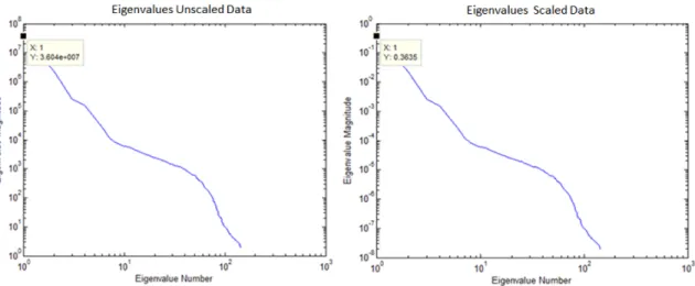
Due to the number of bands and the magnitude of the spectral values, in some cases HSI can present unique issues for algorithms. In particular, the dot products between exemplars often found in kernel methods can grow to be too large in scale. To prevent such scaling issues, the hyperspectral data was also scaled by dividing by the maximum value found across all pixels and all spectra. This maintained the shape and relative magnitude of the signatures, while alleviating computational issues when necessary. Such a technique was also used by Kwon and Nasrabadi [133] when using Kernel Principal Component Analysis (KPCA) for a Kernel Reed-Xiaoli (KRX) algorithm. Scaling by a constant has little effect on eigenvalues and eigenvectors for a covariance matrix when using methods such as PCA (discussed in Section 3.2). Rather, it simply scales the eigenvalues, as for a random variable X and constant c, Var(cX) = c2Var(X). This effect on the eigenvalues is shown in Figure 2.6. This can cause its own problems, however. The scaled values can become too small for an intended purpose, if trying to use a fixed magnitude-based cut-offfor dimension reduction, or the scaled data can become small enough that it causes precision error in the estimation of the eigenvalues and eigenvectors. In any results shown, it is made clear during discussion which version of an HSI dataset is being used, along with any adjustments that had to be made. Alternatively, the data could be standardized. However, that would change the relative information amongst features and thus the relative spectral signatures.
2.3.1.3 Correlation.
Both spatial and spectral correlation can also present issues for algorithms when working with HSI. Spatial correlation occurs because neighboring pixels may contain
Figure 2.6: ARES1D Covariance Eigenvalues Comparison.
similar materials, and because shapes (versus magnitudes) of pixel spectral signatures are often similar. Consider the 25×25 pixel window and its corresponding correlation matrix shown in Figure 2.7. The window contains brush, road, and vehicle (anomaly) pixels that are all highly correlated.
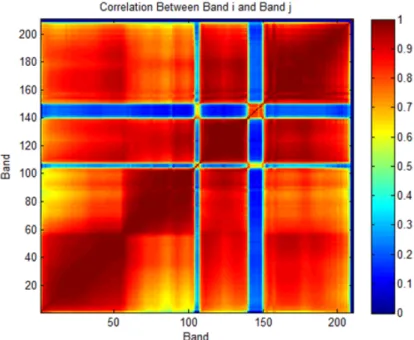
The similar shape of signatures is shown using another sensor and image in Figure 2.8, where 1,000 pixels were randomly sampled. Although different materials have different magnitudes across the bands, the shapes of these signatures are often similar. The spectral correlation for segments of neighboring bands can also be seen using this same Figure. Those bands where the signatures dip to near zero in many cases correspond to absorption bands. Alternatively, when considering the band correlation matrix, shown in Figure 2.9, and referring back to HYDICE data, it can be seen that bands are highly correlated with their neighbors with some exceptions when an absorption band occurs or a certain new range of the spectrum is reached. The segments just mentioned in the pixel signatures become obvious from this matrix. Miller [160] used this property to determine a reduced
(a) Window. (b) Pixel Correlations.
Figure 2.7: ARES1D Window Correlation.
Figure 2.9: ARES1D Band Correlation.
Window-based detection methods can suffer as a result of spatial correlation, as background estimates may be based on pixels that look very much like anomalies. On the other hand, spectral correlation can serve to mask subtle differences between anomalies and non-anomalies.
2.3.1.4 Truth Masks.
As the real-world size of a pixel increases, so too does the likelihood that more than one material is contributing to that pixel’s signature. That is, at higher altitude the sensor is more likely to include several materials within one captured pixel. Therefore, an observed pixel signature may, in fact, be a combination of a number of endmember spectra, or several sub-pixel materials. This possibility can present difficulties in the generation of a truth mask for such images. As a result, the archival truth masks for the ARES HYDICE and HyMAP images reflect such sub-pixel or border anomalous pixels, in addition to the true anomalous
positives or false positives, making comparisons to previous results or algorithms difficult. In order to standardize how these identified pixels are treated, they are investigated in detail in Section 4.3.
2.3.2 HYDICE-Derived.
It should be noted that some of the data sets used have been passed on by previous researchers. Therefore, in some cases these may be sub-images of an original image and the origin truth masks presented may be a previous researcher’s interpretation. Graphics or metrics are included as often as possible to provide clarification.
The Hyperspectral Digital Imagery Collection Equipment sensor-derived (HYDICE) images have 210 spectral bands, between 0.397 and 2.5 µm, including visible through short-wave infrared data. Images from this sensor used here are forest or desert-dominated scenes. The HYDICE ARES1C and ARES2C images are from a rural environment with no specific man-made objects of interest. Their corresponding natural images are shown in Figure 2.10.
(a) ARES1C. (b) ARES2C.
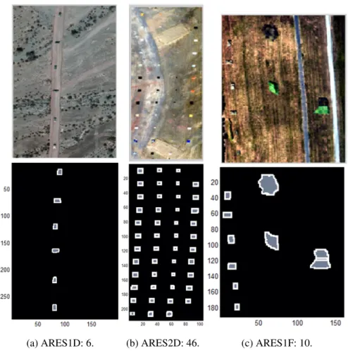
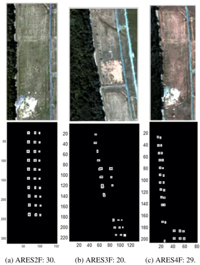
Nearly all of the remaining HYDICE-derived images used are from the Desert radiance II (D) and Forest radiance I (F) collection events. The corresponding set of natural images is shown in Figures 2.11 and 2.12. Most of these images also had target border/neighborhood pixels in their truth masks, depicted here in white. Again, this issue and the proposed resolution is further discussed in Section 3.13.
(a) ARES1D: 6. (b) ARES2D: 46. (c) ARES1F: 10.
Figure 2.11: Three HYDICE Images and Number of Targets.
(a) ARES2F: 30. (b) ARES3F: 20. (c) ARES4F: 29.
Figure 2.12: Three HYDICE Images and Number of Targets.
eight and final five pixel columns from the original image are removed, as they erroneously contain only zero values. The natural image and its truth mask are shown in Figure 2.13. Also shown is one of a few bands in the data where an artifact zero-line occurs. These were retained going into the analysis found in Section 4.5, despite this issue, with the un-derstanding that it would only make classification more difficult. This image is used due to the amount of targets and their close proximity, yielding potential issues for window-based methods. A summary of the HYDICE images is shown in Table 2.1, where anomalous pixels do not include border pixels.
(a) Natural. (b) Truth: 79 Targets. (c) Artifact Line.
Figure 2.13: HYDICE run03m20.
2.3.3 AVIRIS.
The Airborne Visible/Infrared Imaging Spectrometer (AVIRIS) data sets are used courtesy of the National Aeronautics and Space Administration (NASA) and the Jet Propulsion Laboratory of the California Institute of Technology. AVIRIS images contain 224 spectral channels between 0.4 and 2.5µm.
Three Deepwater Horizon images are used, each with associated truth masks developed to correspond with man-made objects in the scene. Scene1 contains 23 targets and is from run f100517t01p00r11rdn b sc01 ort img. Ship1 contains 6 targets and is
Table 2.1: HYDICE Image Properties.
Image Dimensions Pixels Anomalies Anomalous Pixels Border Pixels ARES1C 203×108 21,924 0 0 0 ARES2C 124×198 24,552 0 0 0 ARES1D 291×199 57,909 6 235 437 ARES2D 215×104 22,360 46 523 1942 ARES1F 191×160 30,560 10 1,007 973 ARES2F 312×152 47,424 30 307 1221 ARES3F 226×136 30,736 20 145 314 ARES4F 205×80 16,400 29 109 339 run03m20 960×299 287,040 79 8,255 0
runf100929t01p00r13rdn b sc01 ort img. A fourth AVIRIS image of the Virgin Islands is used, depicting 14 targets from runf051219t01p00r14c sc01 geo img. These four images were chosen for the purposes of variety and due to their varying sizes. They also provide a contrast in scene type relative to the HYDICE imagery. The natural images and their truth masks are shown in Figure 2.14. A summary for the AVIRIS images is shown in Table 2.2.
2.3.4 Pavia.
The Pavia data sets are two scenes acquired by the ROSIS sensor during flights over Pavia in northern Italy and were provided by the Telecommunications and Remote Sensing Laboratory of Pavia University [1]. These provide an investigation of urban scenes from a non-HYDICE sensor with ground truth. The Pavia Centre scene is 1096 ×715 pixels and contains 102 bands, while the Pavia University scene is 610×340 pixels and contains
(a) Scene1. (b) Ship1. (c) 4Ships2. (d) VirginIslands1.
Figure 2.14: AVIRIS Images.
Table 2.2: AVIRIS Image Properties.
Image Dimensions Pixels Anomalies Anomalous Pixels
Scene1 720×707 509,040 23 887
Ship1 657×640 420,480 6 1,025
4Ships2 709×526 372,934 4 332
VirginIslands1 144×163 23,472 14 80
103 bands. The bands in both images are between approximately 0.43 and 0.86 µm [5]. In the Pavia Centre image, two collection areas are joined at line 223. The geometric resolution is 1.3 m, and each image contains a set of nine determined classes and an
In the case of the Pavia Centre scene, the background, water, and meadows classes dominate the scene as approximately 95% of the scene. There is no true outlier class, with remaining classes having between 2600 and 9200 pixels each. The Pavia Centre scene, ground truth, and a small subset of randomly sampled class signatures are shown in Figure 2.15. The Pavia University scene similarly has no true outlier class, however, when analyzing the signatures it becomes apparent that classes such as trees, shadows, or painted metal sheets might be treated as the outlier class (where in the Pavia University image these have 3,064, 947, and 1,345 pixels, respectively). This scene, its ground truth, and a small subset of randomly sampled class signatures are shown in Figure 2.16. It is important to note, as depicted in these figures, the limitations of the given ground truth masks. In the Pavia University image, some labeled pixels, to include some background, have signatures that more resemble other classes. This may be due to sub-pixel traits and simply the complication of labeling each pixel for an image taken over such a large area. Figure 2.17 depicts two of the image’s bands, representative of many of the bands, where certain pixels that are labeled as self-blocking bricks or background in the truth mask have much higher radiance values than their within-class counterparts. Further, when comparing the asphalt signatures between the two images, it can be seen from Figures 2.15 and 2.16 that the asphalt class behaves somewhat differently. This may be, in part, due to the apparent altitude difference. Specific class memberships are shown for each image in Table 2.3.
2.3.5 SpecTIR.
Three radiance data sets from SpecTIR Advanced Hyperspectral and Geospatial Solutions are used in this research [6]. Reflectance hypercubes are also available with CO2
Table 2.3: Pavia Sets Truth Data.
Class Pavia Univ Number Pixels Pavia Centre Number Pixels
Background 164624 635488
Asphalt 6631 3090
Meadows 18649 42826
Gravel 2099
Trees 3064 7598
Painted Metal Sheets 1345
Bare Soil 5029 2863 Bitumen 1330 6584 Self-Blocking Bricks 3682 2685 Shadows 947 7287 Water 65971 Tiles 9248
Figure 2.15: Pavia Centre Scene.
Figure 2.16: Pavia University Scene.
in comparison to those used for the HYDICE and AVIRIS images, and are also arguably less unique among different materials.
The first dataset is a 600×320-pixel urban and mixed environment image of Reno, NV with no associated truth mask. Values are over 356 spectral channels covering approximately 0.39-2.45 µm [6]. The second image also has no associated ground truth for objects or signatures, and was collected as a target of opportunity over the oil spill crisis in the Gulf of Mexico on June 6, 2010. The scene is 1160×320 pixels. The image is radiance collected at 2.2 m ground sample distance, over 360 spectral channels covering
Figure 2.17: Pavia University Bands.
0.39-2.45µm. The third image is an aquatic and coral reef sample over the Red Sea in Saudi Arabia, 600×960 pixels in size. Radiance values are over 128 spectral channels covering approximately 0.39-1µm. The natural images are shown in Figure 2.18. Apparent objects, and/or crests of the spill can be seen in the Oil Spill image, while the coral reef can be seen in the Red Sea image.
(a) Reno. (b) Oil Spill. (c) Red Sea.
2.3.6 HyMap.
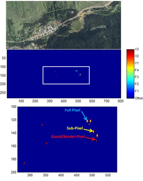
The HyMap sensor data sets were released for the Target Detection Blind Test project [194]. The scene is a 280×800-pixel image of Cooke City in Montana, USA over 126 bands with wavelengths from 0.453 to 2.496µm and an approximate ground sampling distance of 3 m. Two data sets were provided: a self-test with truth/regions of interest of target placement and a blind test with no truth for target placement. Here,the self-test radiance dataset is used. Three vehicles types and four fabric panel colors with known signatures were used for targets. Thus, these pixels are ideal for a matching scenario, but here are also used as a reference for anomaly detection. Admittedly, this is limited in that the rural town is not a clean background and there may have been other vehicles present in addition to what was given as truth. The natural image and truth mask are shown in Figure 2.19. Defined regions of interest, noted here all as target pixels, include full-pixel, sub-pixel, and border pixels for a total of 145 target pixels. Similar to the HYDICE ARES images, these potential target pixels are further investigated in Section 4.3 to form the final truth data used in this research.
Next, in Chapter 3, general methods are discussed that recur throughout the remainder of the research. These methods include dimension reduction techniques, clustering techniques, and existing anomaly detection algorithms. Specific considerations for their application to the data sets presented in this chapter are discussed.
III. General Methods
For consistency of this document, some upfront notation is necessary. Let the hyperspectral data cube be denoted as am×n×parray with pspectral values for each of the
m×n=Nspatial locations, or pixels, of the image. For other multivariate data, letpdenote the number of features and N the number of exemplars, where the data matrix is N × p.
Cdenotes a covariance matrix, andK a Gram matrix, unless otherwise stated. kdenotes a number of centroids, neighbors, or exemplars being used within certain algorithms, or if it is used as a function, denotes the kernel function. 1denotes a vector of ones.
3.1 General Dimension Reduction Techniques
Table 3.1 depicts properties of many dimension reduction techniques as taken from van der Maaten and van den Herik [149]. In the table,ldenotes the number of local models in a mixture,ddenotes the target dimension, iis the number of iterations,wis the number of weights, andris the ratio of nonzero elements to total elements.
There are many linear and non-linear dimension reduction techniques, but Principal Component Analysis (PCA), Kernel PCA (KPCA), and Local Linear Embedding (LLE)-based techniques were explored in this research due to their accessibility and likeness to other methods. For instance, classical multi-dimensional scaling (MDS) using Euclidean distance for dissimilarity is related to PCA in that the MDS coordinates are the component scores from PCA [61]. Isomap, LLE, Laplacian Eigenmaps, and Maximum Variance Unfolding (MVU) can all be considered cases of KPCA using a specific kernel function due to their relation to the more general problem of learning eigenfunctions [149]. Some of these methods are related in that they involve building adjacency matrices based on nearest neighbors. LLE has shown great resemblance to MVU in the mappings produced, and diffusion maps witht= 1 are very similar to KPCA with a Gaussian kernel [149]. In fact,
Table 3.1: Dimension Reduction Technique Properties [149].
Technique Convex Parameters Computational Memory
Principal Component Analysis (PCA) Y None O(p3) O(p2)
Multi-Dimensional Scaling (MDS) Y None O(N3) O(N2)
Isomap Y k O(N3) O(N2)
Max Variance Unfolding Y k O((Nk)3) O((Nk)3)
Kernel PCA (KPCA) Y kernel O(N3) O(N2)
Diffusion Maps Y σ,t O(N3) O(N2)
Autoencoders N netsize O(iNw) O(w)
Local Linear Embedding (LLE) Y k O(rN2) O(rN2)
Laplacian Eigenmaps Y k, σ O(rN2) O(rN2)
Hessian LLE Y k O(rN2) O(rN2)
Local Tangent Space Analysis Y k O(rN2) O(rN2)
Locally Linear Coordination N l,k O(ild3) O(Nld)
any technique that uses the eigen-pairs of a matrix of similarities or dissimilarities between exemplars can be related to KPCA.
Van der Maaten, Postma, and van den Herik [149] did a comparative study of many local and global dimension reduction techniques on a small variety of artificial and natural data sets, and found local techniques to suffer from issues due to large dimensionality, erroneous manifold assumptions, and the scale of eigenvalues complicating eigenproblems. Some global methods suffered similar issues, while the criticality of parameter choice such as with the correct kernel for KPCA, was highlighted.
3.2 Principal Component Analysis
Principal Component Analysis (PCA) generates a set of orthogonal vectors, any subset of which can be used to project into a subspace and where each vector accounts for some portion of the variance found in the data. Let ˆX denote the centered data. Then the principal components are found by eigen-decomposing the covariance matrixC = 1
NXˆ
TXˆ as C = VΛVT, where Λ is the diagonal matrix of eigenvalues of C and V is the matrix of eigenvectors ofC [68]. The eigenvector corresponding to the largest eigenvalue is the linear combination of original features that accounts for the most variance. Additionally, the eigenvector corresponding toλiaccounts for the percentage
λi
Pp
i=1λi
of the total variance found in the data. As a result of these properties and after sorting by eigenvalue magnitude, a number of leading eigenvectors are often chosen so as to account for some percentage of the total variance. The chosen eigenvectors, or components, are then a projection matrix
W. Assuming some subset of the eigenvectors was chosen, this matrix can be used to approximately reconstruct the data, and squared residuals can be found for each exemplar using the row sums of the matrix,
ˆ
where ◦ denotes the Hadamard product. The projection of the data onto the principal components, or set of scores, is simply ˆXW. The correlation of these scores with the original features yields a loadings matrix that represents the degree to which each component correlated with each feature [59].
In application to multi-spectral imagery, Green, et al. [80] investigated component Signal-to-Noise ratios of Airborne Thematic Mapper simulator data. They noted no definite trend relative to increasing noise with increasing component number once the components were ordered by eigenvalue magnitude. In order to generate ordered components in terms of image quality, they developed the maximum noise fraction (MNF) transformation, which is PCA-based but requires good estimates for the signal and noise covariance matrices.
Cheriyadat and Bruce [54] argued that PCA is not the optimal method for feature extraction in target detection applications. Specifically, they noted poor classifier performance on major components when within-class scatter dominated between-class scatter, where factors such as natural variation in the target material, environmental conditions, and sensor angle could cause such large within-class variance. Additionally, they argued that PCA may be poor in the multi-class case as local discriminatory statistics may be ignored. Their suggestions for alternatives required supervision, and they assumed that only major components (largest variance) were being used and that no additional techniques were applied to the component scores [54]. Their arguments raise valid concerns however, that are addressed beginning in Chapter 6. That is, how can good discriminatory components or mappings be selected, and how might information found from PCA and other techniques be fused such that those local discriminatory statistics are not lost?
3.3 Kernel Principal Component Analysis
One non-linear form of PCA uses kernels to perform standard PCA in a higher-dimension feature space F. This enables a similar process for data with a non-linear
Φ: Rp →Rd, whered > p. This mapping sends the original data into an arbitrarily large, possibly infinite dimensional space. In this space, each centered exemplar is defined as,
ˆ Φ xj = Φ xj − 1 N N X i=1 Φ(xi), (3.2)
for all j. The covariance matrix is then also,
C = 1 N N X j=1 ˆ Φ xj ˆ Φ xj T . (3.3)
To perform linear PCA in this space, eigenvaluesλand eigenvectorsvare solved for in the higher dimensional space using the eigenproblemλv = Cv[97, 200]. This implies that for any exemplarxk ∈Rp,
λ
ˆ
Φ(xk)·v
=Φˆ(xk)·Cv. (3.4)
Each eigenvector vis a linear combination of the training exemplars in the new centered space, v= N X j=1 αjΦˆ(xj). (3.5)
Using Equations 3.3 and 3.5 in 3.4 yields for everyk =1, . . . ,N,
λX j αjΦˆ(xk)·Φˆ(xj)= 1 N X j αj X i {Φˆ(xk)·Φˆ(xi)}{Φˆ(xi)·Φˆ(xj)}. (3.6)
But defining ˆKi j = Φˆ(xi)·Φˆ(xj) andα=(α1. . . αN)T, this simplifies to, λα= 1
NKˆα→ (Nλ)α= Kˆα. (3.7)
Therefore, if the dot products can be found, the eigenvalues Nλand eigenvectors α can be derived directly from ˆK andΦdoes not need to be known. In fact, the dot products are found using a kernel function. ˆK is the modified, or centered form of the Gram matrix
K, where Ki j =
D
Φ(xi),Φ(xj)E = k(xi,xj) for some kernel function k. Recalling that an entry in ˆK is just the dot product of two vectors as found in Equation 3.2, by algebraic reduction it can be shown that ˆK can be found fromK as,
ˆ
where1N is aN ×N matrix with values 1/N [200]. This subtracts the column means and the row means, and adds back the overall mean.
Because F is higher-dimensional than the original data, only non-zero eigenvalues should be considered. In order to normalizeα, non-zerovare required to be normalized as
v(l)·v(l)= 1. Using equation 3.5 in this equation simplifies to the normalized coefficients,
ˆ
α(l)= α (l) √
(Nλl). (3.9)
To clarify, only αˆ and ˆK are needed to project onto v. This can be shown easily by considering that for some test datay,
v(l)·Φˆ(y)= N X i=1 ˆ α(l) i ˆ Φ(xi)·Φˆ(y)= N X i=1 ˆ α(l) i Kˆ test (xi,y), (3.10)
where ˆKi jtestis the similarly centered form ofk(yi,xj). This is performed as, ˆ
Ktest = Ktest−1MNK−Ktest1N +1NMK1N, (3.11) where1M
N isM×N with all entries 1/N, for a test set with Mexemplars [200].
One lingering question is what constitutes a kernel. To define this, Mercer’s theorem is used [161]. Mercer’s theorem states that a symmetric functionk(x,y) can be expressed as an inner product,
k(x,y)=hΦ(x),Φ(y)i (3.12) for someΦif and only ifk(x,y) is positive semidefinite,
Z k(x,y)g(x)g(y)dxdy≥ 0,∀g∈L2 (3.13) or equivalently, k(x1,x1) k(x1,x2) . . . k(x2,x1) ... (3.14)
is positive semi-definite for any collection {x1, . . . ,xN} of exemplars [113]. That is, the Gram matrix is positive semi-definite for the set of data.
Some commonly used Mercer kernels include, 1. Polynomial: (x·y+c)d, wherec∈R,d ∈N, 2. Sigmoid: tanh(x·y+c), wherec∈R, 3. Inverse Multiquadric: p 1
kx− yk2+σ2, for a given norm,
4. and the Gaussian/Radial Basis Function: exp −kx−yk 2
2σ2 !
,
using theL2norm wherecis some real constant,d ∈Nis the power, andσ >0 is the spread
parameter [146]. Within the context of KPCA, use of the Gaussian kernel only makes the Normality assumption in the higher-order space, and not the originating space. The dot product x· yis also a kernel, referred to as the linear kernel, but is closely tied to normal PCA. If (λi,vi) are an eigen-pair for XTX, thenλi andui = λ
−1/2
i Xvi are an eigen-pair for
XXT. Doing PCA in this latter manner, so that scores are computed for variables rather than exemplars, has also been denoted as kernel eigenfaces when doing facial recognition assuming alignment of certain features across the images [224]. Typically with kernel eigenfaces, rather than computing a score for every pixel of an image, each image is reshaped to be treated as a column of pixel values, and thus, the transpose causes each column to be treated as an exemplar. Additionally, kernel eigenfaces differs from strict KPCA in that projected exemplars are often compared against predefined face classes for purposes of classification [162, 206]. Paiva, Xu, and Principe [170] showed that KPCA with a Gaussian kernel provided optimum entropy projections in the input space.

![Figure 3.6: Workflow Diagrams for PCA and PCA Involving Wavelets [87].](https://thumb-us.123doks.com/thumbv2/123dok_us/1282971.2672364/79.918.196.727.272.845/figure-workflow-diagrams-pca-pca-involving-wavelets.webp)
