Is islamic stock related to interest rate ? Malaysian evidence

Munich Personal RePEc Archive

Is islamic stock related to interest rate ?

Malaysian evidence

Abu Bakar, Norhidayah and Masih, Mansur

INCEIF, Malaysia, Business School, Universiti Kuala Lumpur,

Kuala Lumpur, Malaysia

30 September 2016

Online at

https://mpra.ub.uni-muenchen.de/101190/

Is islamic stock related to interest rate ? Malaysian evidence

Norhidayah Abu Bakar1 _{and Mansur Masih}2

Abstract

This study aims to examine the dynamic relationship of Islamic stock price with interest rate and other monetary policy variables by using the standard time series approach. The main objective is to test the Islamic principle whether interest rate (or riba in Islamic term) influences the movement of Islamic stock price. Malaysia is taken as a case study. In addition, the extent of the influence of other variables namely, money supply and inflation in explaining Islamic stock return could be captured. The findings tend to suggest that Islamic stock price appears to be significantly affected by the interest rate and inflation in the long run, but insignificantly affected by broad money supply. Islamic stock price is relatively more sensitive to inflation rate, compared to other variables. The finding implies that Islamic stock is a good hedge against inflation as it tends to react positively to inflation rates

Keywords: Islamic stock, interest rate, VECM, VDC, Malaysia

__________________________________

1 _{INCEIF, Lorong Universiti A, 59100 Kuala Lumpur, Malaysia.}

2 Corresponding author, Senior Professor, UniKL Business School, 50300, Kuala Lumpur, Malaysia. Email: mansurmasih@unikl.edu.my

1.0 Introduction – Issue motivating the study

Islamic stocks in Malaysia are represented by companies that have passed through the shariah

screening criteria set by the Security Commission Malaysia. This indicates that those companies’ operations are not directly related to the main prohibitions in shariah, thus one of them is riba. Therefore, since interest or riba in Islamic term is prohibited under Islamic law, it is important that Islamic investment to be free from the influence of interest either direct (in the operations) or indirect (reflecting in the stock’s price). In addition, Proper understanding of the affecting factors of Islamic stock prices (interest rate, money supply and inflation) is highly crucial for economist, policy makers and investor. Therefore, the exact patterns, interaction and which variable is dominant in the interaction need to be analysed empirically. By this, Islamic investor could justify their source of income, and the industry could somehow measure to what extent Islamic Finance is different from the conventional finance. This study is also meant to contribute further to the literature since empirical study for Islamic equity investment is limited.

2.0 Objectives

This study intends to examine the dynamic relationship of Islamic stock price with interest rate and other monetary policy variables. The main objective of this study is to identify whether interest rate influences the movement of Islamic stock price in Malaysia. In addition to interest rate, other monetary policy variables will also be incorporated in the model. The additional variables will act as the controlled variables, thus the second objective is to capture the degree of influence of other variables namely, money supply and inflation in explaining Islamic stock return.

3.0 Theoretical framework

The incorporation of the selected variables in the analysis is consistent with theoretical foundation that stock price returns are calculated through the stock valuation model which is represented by the discounted present value of future cash flows. Therefore, any changes in monetary variables such as, interest rates and money supply may affect the firm’s cash flows and thus, influence the stock price specifically by affecting the discount factors (Ibrahim and Yusoff,

2001). In addition, changes in stock price may also reflect real economic activities which lead to an increase in demand for real money and interest rate.

Expected relationships among the variables are; first, interest rate is expected to have a negative relationship with stock returns. This is clearly understood based on the stock valuation model that interest rate should act as a discounting factor which will lessen the value of cash flows.

Second, money supply could have either negative or positive relationship with stock return. According to Ibrahim and Yusoff (2001), money supply exerts a positive effect on the stock price in the short run but negatively in long run. The negative relationship is channelled through the impact of increasing interest rate. If the increase in money supply generates inflation as well as contributes to inflation uncertainties then it might exert a negative influence on the stock price. Increase in money supply leads to increase in interest rate and therefore a decrease in stock price. Therefore, money supply can have a positive impact on stock price if the increase in money supply leads to an expansion in economic activities. If this the case, cash flow and stock price will increase.

Third, inflation is like money supply could have either positive or negative relationship with stock price. Previous studies in Malaysia such as Ibrahim (1999), Ibrahim and Yusuff (2001) and Ibrahim and Hassanudden (2003) found that inflation is positively related to stock prices. According to these papers, the positive relationship between stock price and inflation suggest that stock prices are a good hedge against inflation.

4.0 Literature review

Various empirical researches have been done in analysing factors that may impact stock prices. In the case of emerging market such Malaysia several research have add in this line of literature among them are Ibrahim (1999), Ibrahim and Yusuff (2001), Ibrahim and Hassanudden (2003) and Asmy et.al (2009). These four papers investigate the dynamic interactions between

macroeconomic variables and the stock prices for an emerging market such Malaysia, using cointegration and Granger causality tests.

The first paper Ibrahim (1999) analyse the interaction between stock price and seven macroeconomic variables. Industrial production, consumer price index (CPI), narrow and broad money supply M1 and M2, domestic credit aggregates, official reserve and exchange rate as independent variables and Kuala Lumpur Composite Index (KLCI) as the proxy for stock prices. Results from this study suggest cointegration between the stock prices and three macroeconomic variables namely consumer prices, credit aggregates and official reserves.

In the next paper, Ibrahim and Yusoff (2001) analyses dynamic interaction among three macroeconomic variables (real output, price level, and money supply), exchange rate, and equity prices in Malaysia. With the addition of stronger techniques such as impulse response and variance decomposition, their result finds that movements in the Malaysian stock market are driven more by domestic factors, particularly the money supply, than by the external factor (such the exchange rate).

In the third paper, Ibrahim and Hassanudden (2003) analyses dynamic linkages between stock prices (KLCI) and four macroeconomic variables (money supply (M1), consumer price index, industrial production and exchange rate). With the attempt to capture international market effect, two major international stock market indexes were integrated in the research namely US S&P 500 and Japan Nikkei 255 indices from 1977 to 1998 on monthly basis. Empirical results suggest the presence of a long-run relationship between these variables and the stock prices and substantial short-run interactions among them. In particular, suggest positive short-run and long-run relationships between the stock prices and two macroeconomic variables. The exchange rate, however, is negatively associated with the stock prices. For the money supply, documents immediate positive liquidity effects and negative long-run effects of money supply expansion on the stock prices.

Asmy et.al (2009) examine the short-run and long-run causal relationship between Kuala Lumpur Composite Index (KLCI) and selected macroeconomic variables namely inflation, money supply and nominal effective exchange rate during the pre and post crisis period from 1987 until

1995 and from 1999 until 2007 by using monthly data. Consistence with the previous paper, the findings shows that there is cointegration between stock prices and macroeconomic variables. The results suggest that inflation, money supply and exchange rate seem to significantly affect the KLCI. These variables considered to be emphasized as the policy instruments by the government in order to stabilize stock prices.

All of the above papers only focus on conventional stocks market and try to investigate its relationship with selected macroeconomics variables. Currently, Islamic financial system especially in Malaysia is operating side by side with conventional system, therefore as addition and complementary to the above researches, Yusof and Majid (2006, 2007) had explored the stock market volatility in Malaysia for both Islamic and conventional market.

Using the same technique (cointegration and vector autoregression) and with the addition of regression, Yusof and Majid (2007) analyse the stock market volatility in Malaysia and how they are affected to the volatility in monetary policy variables for both Islamic and conventional market. The variables used to measure conventional and Islamic stock market index are Kuala Lumpur Composite Index (KLCI) and Rashid Hussain Berhad Islamic Index (RHBII). While the monetary policy variables used in their study are the narrow money supply (M1), the broad money supply (M3), interest rates (TBR), exchange rate (MYR), and Industrial production Index (IPI). This study finds that stabilizing interest rate would have insignificant impact on the volatility of the Islamic stock market. This study was inline and supports their earlier study (Yusof and Majid, 2006) which finds that interest rate volatility affects the conventional stock market volatility but not the Islamic stock market volatility. Both of these studies highlight the Islamic principles that interest rate is not a significant variable that explain stock market volatility.

In relation to the above, as the theory and empirical answer are controversial, and as another contribution to this line of literature, this paper seeks to explore Islamic stock price movement in case of Malaysia and how it is affected to the monetary policy variables by analysing the newly develop Islamic index which is FTSE Bursa Malaysia Emas Shariah Index (FBMSHA).

5.0 Methodology

This study adopts the standard time series technique in order to serve the research objective of finding empirical evidence in the nature of relations between Islamic stock and interest rates. In short, the methodology employed will begin with (i) unit-root tests (testing the stationarity of variables), (ii) determine the order of the VAR, (iii) applying the Engle-Granger and Johansen cointegration tests, (iv) examines the long run structure modelling (LRSM), (v) conducting the test of vector error correction model (VECM), (vi) applying variance decomposition (VDC) technique, (vii) applying impulse response function (IRF), (viii) and persistence profile (PF).

As explained by Masih (2010), the cointegrating estimated vectors will be subjected to exact identifying and overidentifying restrictions based on theoretical and a priori information of the economy. The test of cointegration is designed to examine the long-run theoretical or equilibrium relationship and to rule out spurious relationship among the variables. VECM is then employed to indicate the direction of Granger causality both in the short and long run. Afterwards, the variance decomposition technique is applied to indicate the relative exogeneity/endogeneity of a variable. The proportion of the variance explained by its own past shocks can determine the relative exogeneity/endogeneity of a variable. The variable that is explained mostly by its own shocks (and not by others) is deemed to be the most exogenous of all. The impulse response function (IRF) will then be applied in order to map out the dynamic response path of a variable due to a one period SD shock to another variable. The IRF is a graphical way of exposing the relative exogeneity or endogeneity of a variable. Finally, the persistence profiles will be applied. They are designed to estimate the speed with which the variables get back to equilibrium when there is a system-wide shock.

5.1 Data

Data employed in this research are time series data, with 62 observations, taken form DataStream which consist of monthly data from 2006 – 2012. FTSE Bursa Malaysia Emas Shariah Index (FBMSHA) had only been introduced starting from 2006 as a replacement to previous shariah index (KLSI). Quoted from Bursa Malaysia, “as announced on 22nd Jan 2007 during the

November 2007, making the FBMSHA the singular benchmark index for Malaysian

Shariah-compliant investments.”

The variables are defined as follows:

FBMSHA : FTSE Bursa Malaysia Emas Shariah Index monthly price, will act as a Proxy for Islamic stock price.

INT : Interest rate (Malaysia KLIBOR one month - offered rate)

M3 : Broad money supply which represents by (M1) currency in circulation and demand deposits, plus (M2) savings deposits, fixed deposits, NIDs, Repos, foreign currency deposits, plus deposits placed with other banking institutions.

INF : Inflation (Monthly CPI)

6.0 Estimations and Discussions

6.1 Testing Stationarity of Variables

Before testing the stationarity of variables, all of the variables will be transformed into log form except for INT (interest rate), as it is naturally in percentage form. Conducting augmented Dickey Fuller (ADF) test on each variables, the result shows that all variables are non-stationary in their level form and, stationary after taking the first difference of their log form (eg: DFBMSHA = LFBMSHA – LFBMSHAt-1). Table 1 below summarizes the results.

Table 1: Augmented Dickey Fuller Stationary test result

Variables Test Statistic Critical Value Implication

Variables in Level Form

LFBMSHA -2.1081 (AIC) -3.489 Non-Stationary

-1.6944 (SBC) -3.489 Non-Stationary

INT -1.6624 (AIC) -3.489 Non-Stationary

-1.3488 (SBC) Non-Stationary

LM3 -1.8918 -3.489 Non-Stationary

Variables in Differenced Form

DFBMSHA -3.2843 (AIC) -2.9137 Stationary

-4.9386 (SBC) -2.9137 Stationary

DNT -3.3537 -2.9137 Stationary

DM3 -4.5569 -2.9137 Stationary

DINF -4.2638 -2.9137 Stationary

The highest ADF regression order based on computed value for AIC and SBC were used in determining which test statistic to compare with the 95% critical value for the ADF statistic. As described in the above results, all of the variables used for this analysis are I(1). Note that in some cases, AIC and SBC produce different orders, therefore, we have taken different orders and compared both (for example, this applies to the variable DFBMSHA). This is not an issue as in all cases as the implications of both are consistent.

ADF test of stationary only correcting autocorrelation problem. To take care of heteroscedasticity, a more stringent test of stationary which is Phillips Perron (PP) test of stationary has been conducted. (Table 2) Results indicate consistency with ADF test, whereby all variables are non-stationary in their level form and stationary after taking the first difference of their log form. For INT in its level form, the rejection criterion is at 5% significant level.

Table 2: Phillips Perron Stationary test result

Variables Coefficient (S.E) T-Ratio [P-Value] Implication

Variables in Level Form

LFBMSHA -.070053 (.046434) -1.5086[.137] Non-Stationary INT -.035036 (.020851) -1.6803[.098] Non-Stationary LM3 .1853E-3 (.010642) .017412[.986] Non-Stationary LINF -.016565 (.020954) -.79056[.432] Non-Stationary

Variables in Differenced Form

DFBMSHA -.90300 (.16600) -5.4397[.000] Stationary DINT -.57781 (.065835) -8.7766[.000] Stationary DM3 -.85317 (.088666) -9.6223[.000] Stationary DINF -.54812 (.061553) -8.9048[.000] Stationary

6.2 Determination of the order (or lags) of the VAR model

The next task is to determine the order of VAR, which the number of lag to be used. As presented in table 3, based on the p-value of adjusted LR and the highest AIC and SBC, the result suggest that the optimum order of VAR is 1. (See Appendix 2 for details)

Table 3: Determination of order of VAR

Order AIC SBC Adjusted LR Test

0 496.39 492.34 113.68 [0.105]

1 501.28 481.03 90.55 [0.197]

2 492.36 455.91 82.71 [0.058]

3 496.84 444.18 108.46 [0.114]

6.3 Testing Cointegration

Cointegration is the test to see whether all variables move together or integrated in the long term. This indicates the theoretical relationships among variables. Applying Engle-Granger cointegration test (Table 4), result indicates that all of the variables are cointegrated in the long run. However Engle-Granger test could only identify one cointegrating vector. To strengthen the result, standard Johansen cointegration test was applied, (Table 5) the result shows that the variables have one cointegrating vector at 95% confidence level on the basis of maximal Eigen value and trace statistics.

Table 4: Engle-Granger result for cointegration

Specification _LINF

t= α + β1LFBMSHAt+ β2LINTt+ β3LM3t+ 𝑒𝑡

Test Statistics Critical Value Implication

ADF(2) -4.5141 -4.3064 Cointegrated

Table 5: Johansen ML result for multiple cointegration

Ho H1 Test Statistic 95% Critical 90% Critical

Maximum Eigenvalue Statistics

r = 0 r>= 1 49.9264 31.7900 29.1300

r<= 1 r>= 2 18.1494 25.4200 23.1000

Trace Statistics

r = 0 r>= 1 83.5191 63.0000 59.1600

An evidence of cointegration implies that the relationship among the variables is not spurious, which suggest that there is a theoretical relationship among the variables and that they are in equilibrium in the long run. This result has a strong implication on this study, whereby it indicates that the Islamic stock price and interest rate together with other monetary variables (money supply and inflation) are theoretically integrated in the long run. However, to make the coefficient of the integrating vector consistent with the theory, the next procedure which is LSRM need to be applied.

6.4 Long Run Structural Modelling (LRSM)

In line with the objective of this paper, which to identify the relationship of Islamic stock price, interest rate and monetary variables, we first imposed a normalizing restriction of unity on the FBMSHA variable at the ‘exactly identifying’ stage (see Panel A of Table 6). As tabulated, in exact identification, M3 proves to be insignificant among all other variables in explaining FBMSHA. Experimented with a restriction of unity on the broad money supply (M3) variable at the ‘overidentifying’ stage (Panel B of Table 6) by imposing overindentifying restriction on the coefficient of M3, the result which presented by chi-square statistics (0.0254[.873]) indicates that the null is accepted thus the restriction is correct. This indicates that only interest rate and inflation has significant role in explaining Islamic stock price.

Table 6: Exact and over identifying restriction on the cointegrating vector

Variable Coefficient Standard Error t-Ratio

Panel A: Exact Identification

LFBMSHA 1.0000 None None

INT -0.0955 0.0356 -2.6826*

LM3 0.1985 1.2492 0.1589

LINF 7.4280 1.5738 4.7198*

Trend -0.0204 0.0089 2.2728*

Panel B: Over-identification

LFBMSHA 1.0000 None None

INT -0.0949 0.0354 -2.6835*

LM3 0.0000 None None

LINF 7.5121 1.4800 5.0757*

Trend -0.0191 0.0032 5.9839*

6.5 Vector Error Correction Model (VECM)

The analysis thus far, had established that there are three variables cointegrated to a significant degree (Islamic stock price, interest rate, and inflation). The next aim is to proceed with VECM in order to identify the direction of Granger causality as to which variable is leading and which variable is lagging (i.e. which variable is exogenous and which variable is endogenous). (Table 7) Looking at the significant of error correction coefficient, FBMSHA, INT and INF appeared to be endogenous and M3 is exogenous. That tends to indicate that Islamic stock price response to broad money supply, but not by the opposite. The error correction term in the FBMSHA equation is significant. It implies that the deviation of the variables (INT, M3 and INF), which represented by the error correction term, has a significant effect on the Islamic stock price variable that bears the burden of short-run adjustment to bring about the long-term equilibrium.

Table 7: Error correction model (See Appendix 5.1 -5.4 for details)

DFBMSHA DINT DM3 DINF

ECM (-1) -4.7556[.000]* 3.6006[.001]* -.46788[.642] 2.2060[.031]*

Implication Endogenous Endogenous Exogenous Endogenous

Chi Sq Serial Correlation (1) .31469[.575] 4.0031[.045] 1.3705[.242] 10.0232[.002] Chi Sq Functional Form (1) 5.4457[.020] 11.0761[.001] .02375[.878] .004198[.948] Chi Sq Normality (2) 9.5584[.008] 289.813[.000] 2.5297[.282] 2046.0 [.000] Chi Sq Heteroscedasticity (1) 1.4982[.221] 14.1930[.000] .33214[.564] 0.23331[.629] Notes: Due to the chosen order of VAR equal to 1, the equations do not capture the short term coefficient among variables. P-values are given in parenthesis. * Indicates significant at 5%

The diagnostics of all the equations of the error correction model (testing for the presence of autocorrelation, functional form, normality and heteroskedasticity) tend to indicate that the equations contain some problems, but we decided to proceed with estimation. We also checked the stability of the coefficients by the CUSUM and CUSUM SQUARE tests (Figure 1), which indicate that they are stable.

Figure 1: Plot of cumulative sum of recursive residuals and plot of cumulative sum of squares of recursive residuals

6.6 Variance Decompositions (VDCs): Orthogonalized and Generalized

Even though VECM has indicated the endogeneity/exogeneity of a variable, it does not able to screen out the relative degree of endogeneity or exogeneity of the variables. To detect this, variance decomposition technique will be used. The relative exogeneity or endogeneity of a variable can be determined by the proportion of the variance explained by its own past. The variable that is explained mostly by its own shocks (and not by others) is deemed to be the most exogenous of all. In table 7 for orthogonalized and table 8 for generalized, at the end of the forecast horizon number ten, the contributions of own shocks towards explaining the forecast error variance of each variable are indicating a consistence result. M3 is the most exogenous, the rank of three endogenous variables are INF, followed by INT and FBMSHA. The result depict that M3 is the most exogenous thus comply with VECM result as the leading variable.

-20 -10 0 10 20

II III IV I II III IV I II III IV I II III IV

2008 2009 2010 2011 CUSUM 5% Significance -0.4 -0.2 0.0 0.2 0.4 0.6 0.8 1.0 1.2 1.4

II III IV I II III IV I II III IV I II III IV

2008 2009 2010 2011

Table 7: Percentage of forecast variance explained by innovations in Orthogonalized variance decompositions

Month DFBMSHA DINT DM3 DINF

DFBMSHA 1 0.83174 0.13340 0.01773 0.01711 5 0.54535 0.13593 0.01483 0.30388 10 0.26976 0.08578 0.00782 0.63662 DINT 1 0.18078 0.79613 0.00294 0.02013 5 0.31767 0.57520 0.00426 0.10285 10 0.37860 0.46200 0.00477 0.15461 DM3 1 0.01613 0.00235 0.97943 0.00208 5 0.00898 0.00179 0.98225 0.00696 10 0.00544 0.00144 0.98136 0.01175 DINF 1 0.04132 0.00227 0.00062 0.95578 5 0.10081 0.00436 0.00016 0.89465 10 0.13733 0.00558 0.00014 0.85694

Table 8: Percentage of forecast variance explained by innovations in Generalized variance decompositions

Month DFBMSHA DINT DM3 DINF

DFBMSHA 1 0.97088 0.00195 8.10E-05 0.02708 5 0.58818 0.02763 0.001146 0.38304 10 0.27867 0.04841 0.002007 0.67092 DINT 1 0.22013 0.76831 3.45E-05 0.01152 5 0.42875 0.48673 2.52E-04 0.08426 10 0.52443 0.33953 4.06E-04 0.13563 DM3 1 0.01646 9.02E-06 0.98332 2.08E-04 5 0.00909 1.22E-04 0.98867 0.00210 10 0.00547 2.71E-04 0.98986 0.00439 DINF 1 0.04300 0.00100 0.00285 0.95314 5 0.10832 0.00350 2.65E-03 0.88552 10 0.14976 0.00522 0.00252 0.84249

The main difference between orthogonalized and generalized is, in orthogonalized it depends on the particular ordering of the variables in the VAR and assumes that when a particular variable is shocked, all other variables in the system are switched off, whereby in generalized, no such assumption are made. Intuitively, generalized method is more coherent with the real world. As for that, the result for generalized VDC the percentage of variable explained by its own shocked are: FBMSHA (29%), INT (34%), M3 (99%), and INF (82%). As the main focus of the paper, FBMSHA only explained by INT by 4.8%, where most of the Islamic stock index is explained by INF (67%) and the least is M3 (0.2%).

6.7 Impulse Response Functions (IRFs)

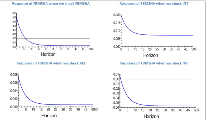
In VDC, the purpose is to see the degree of dependency of the variable to itself to determine relative endogeneity and exogeneity of the variables. While, in IRF, the main concern is to see the impact on others when one variable is shock. As in VDC, the shock can be orthogonalized and generalized. Referring to the IRF graphs (figure 1 and figure 2), the result is consistent with VDC, which indicates FBMSHA is relatively more sensitive to a 1% SD shock to the inflation compared to interest rates and broad money supply.

Response of FBMSHA when we shock FBMSHA Response of FBMSHA when we shock INT

Response of FBMSHA when we shock M3 Response of FBMSHA when we shock INF

Figure 2: Orthogonalized impulse Response of FBMSHA to one S.E shock in the equation for FBMSHA, INT, M3 and INF (See Appendix 7.1 for details)

one S.E. shock in the equation for L

Horizon -0.01 -0.02 0.00 0.01 0.02 0.03 0.04 0.05 0.06 0 5 10 15 20 25 30 35 40 45 5050

one S.E. shock in the equation for

Horizon 0.000 0.005 0.010 0.015 0 5 10 15 20 25 30 35 40 45 5050

one S.E. shock in the equation for

Horizon 0.0000 0.0005 0.0010 0.0015 0.0020 0.0025 0.0030 0 5 10 15 20 25 30 35 40 45 5050

one S.E. shock in the equation for L

Horizon -0.01 -0.02 -0.03 -0.04 -0.05 -0.06 0.00 0 5 10 15 20 25 30 35 40 45 5050

Response of FBMSHA when we shock FBMSHA Response of FBMSHA when we shock INT

Response of FBMSHA when we shock M3 Response of FBMSHA when we shock INF

Figure 3: Generalized impulse Response of FBMSHA to one S.E shock in the equation for FBMSHA, INT, M3 and INF (See Appendix 7.2 for details)

However, when we shock FBMSHA, the highest impact would be towards INT, and the same case implies when we shock INT the highest impact is towards FBMSHA as compared to the others (figure 4 and 5). This implies a strong relationship between those two. The orthogonolized and generalized IRF tend to implies identical results.

Responses of INT, M3 and INF when we shock FBMSHA Responses of FBMSHA, LM3 and INF when we shock INT

Figure 4: Orthogonalized impulse Response to one S.E shock in the equation for FBMSHA and INT (See Appendix 7.1 for details) Horizon -0.01 -0.02 0.00 0.01 0.02 0.03 0.04 0.05 0.06 0 5 10 15 20 25 30 35 40 45 5050 Horizon 0.000 0.005 0.010 0.015 0.020 0 5 10 15 20 25 30 35 40 45 5050 Horizon 0.000 0.002 0.004 0.006 0.008 0 5 10 15 20 25 30 35 40 45 5050 Horizon -0.01 -0.02 -0.03 -0.04 -0.05 -0.06 0.00 0.01 0 5 10 15 20 25 30 35 40 45 5050

one S.E. shock in the equation for LFBMS

LFBMSHA INT LM3 LINF Horizon -0.05 0.00 0.05 0.10 0.15 0.20 0 5 10 15 20 25 30 35 40 45 5050 LFBMSHA INT LM3 LINF Horizon -0.05 0.00 0.05 0.10 0.15 0 5 10 15 20 25 30 35 40 45 5050

Responses of INT, M3 and INF when we shock FBMSHA Responses of FBMSHA, M3 and INF when we shock INT

Figure 5: Generalized impulse Response to one S.E shock in the equation for FBMSHA, INT, M3 AND INF (See Appendix 7.2 for details)

6.8 Persistence Profiles (PF)

Persistence Profiles is a system-wide shock, where the shock comes from the external source to the cointegrating vectors, and it shows the time horizon required for variables to get back to equilibrium. Referring to the graph, it indicates that the system would take approximately 13 months for the cointegrating relationship to return to equilibrium.

Figure 6: Persistence profile of the effect of a system-wide shock

7.0 Conclusions

7.1 Main findings

This study attempts to establish the link between Islamic stock price, interest rate and other two monetary policy variables (money supply and inflation rate) in Malaysia. To realize this, the time series method is employed.

S.E. shock in the equation for LFBMSHA

LFBMSHA INT LM3 LINF Horizon -0.05 0.00 0.05 0.10 0.15 0.20 0 5 10 15 20 25 30 35 40 45 5050

one S.E. shock in the equation for INT

LFBMSHA INT LM3 LINF Horizon 0.00 0.05 0.10 0.15 0 5 10 15 20 25 30 35 40 45 5050

of a system-wide shock to CV'(s

Horizon

The study suggests that interest rate and inflation appear to have significantly affected Islamic stock price in the long run. This study also suggests that interest rate is not the causation in explaining Islamic stock price, since both of them appeared to be endogenous in the estimation. However Islamic stock price and interest rate tend to respond the most if either one of them is shocked. This implies a sort of relationship between the two.

In addition, broad money supply appeared to have an insignificant relationship in explaining Islamic stock price, this is evidenced by LRSM. However, Islamic stock price tends to be relatively more sensitive to inflation rates as compared to the others with positive relation. This is evidenced by VDC and later supported by IRF. Numerically in VDC, Islamic stock price is only explained by interest rate by 4.8%, whereas most of the Islamic stock price is explained by inflation (67%) and the least is M3 (0.2%).

7.2 Policy Implications

The finding of this study is to contradict Yusof and Majid, 2006 and 2007 in highlighting the tenet of Islamic principles that interest rate is not a significant variable in explaining stock market return. As a result, the uniqueness of the Islamic stock which is represented by Shariah-compliant companies does not suffice. The investors need to be cautious with interest rate movement as it is statistically significant in affecting Islamic stock price, thus act as a discount factor to the return. The finding also implies that Islamic stock is a good hedge against inflation as it tends to react positively to inflation rates (Ibrahim, 1999, 2003).

7.3 Limitations

This study contains some limitations mainly due to the limitations on the availability of data. As mentioned before, analysis conducted in this paper taking data starting from the introduction of FMBSHA (March 2006 - January 2012), which is roughly five years. Five years in the industry can be considered as the infancy stage of development. Almost all research paper in this literature (Ibrahim, 1999, 2003) collect data for at least 20 years. The implication of this, may lead to the bias of result, where the result may only represent the current economic situation. As mentioned by Ibrahim (1999), changes in the stock price will depend not only on the changes in macroeconomics variables but also on the long term relationship between them. Therefore the

actual trend which involves long term relationship could not be captured. Therefore it is suggested here that further research needs to be done to capture the real interaction after 10 or 15 years from now.

On top of that, this paper only focuses on Islamic stock price, hence, further research is suggested to analyse both Islamic and conventional stocks return. This is for the purpose of making comparison, thus the whole picture and the uniqueness of Islamic stock if any, could be pictured. In addition to this, to capture international market effect, major international Islamic stock market indexes such as, Dow Jones Islamic Index could be integrated into the research.

References

Engel, R. F., and Granger, C. W. (1987), Cointegration and error-correction

representation, estimation, and testing, Econometrica, 55(2), 251–276.

Hussin, M., Muhammad, F., Abu, M. and Awang, S. (2012), Macroeconomic Variables and

Malaysian Islamic Stock Market: A time series analysis, Journal of Business Studies Quarterly,

3(4), 1-13.

Ibrahim, M. H. (1999), Macroeconomic variables and stock prices in Malaysia: An empirical analysis. Asian Economic Journal, 13(2), 219-231.

Ibrahim, M. H. and Aziz, H. (2003), Macroeconomic Variables and Malaysian Equity Market: A View through Rolling Subsamples. Journal of Economic Studies, 30(1), 6-27.

Islam, M. (2003), The Kuala Lumpur stock market and economic factors: a general to specific error correction modelling test, Journal of the Academy of Business and Economics, 1(1), 37-47.

Johansen, S. and Juselius, K. (1990), Maximum Likelihood Estimation and Inferences on

Cointegration With Application to the Demand for Money, Oxford Bulletin of Economics and

Statistics, 52, 169-210.

Masih, M., Al-Elg, A. and Madani, H. (2009), Causality between financial development and economic growth: an application of vector error correction and variance decomposition methods to Saudi Arabia, Applied Economics, 41, 1691 – 1699.

Masih, M. and Algahtani, I. (2008), Estimation of long-run demand for money: An application of long-run structural modelling to Saudi Arabia, Economia Internazionale (International

Economics), 61(1), 81 – 99.

Maysami, R. and Koh, T. (2000), A Vector Error Correction model of the Singapore stock market,

International Review of Economics and Finance, 9(1),79-96.

Maysami, R. and Sim, H. (2002), Macroeconomics variables and their relationship with stock

returns: error correction evidence from Hong Kong and Singapore, The Asian Economic Review,