Testing for Multiple Bubbles

TESTING FOR MULTIPLE BUBBLES

By

Peter C.B. Phillips, Shu-Ping Shi, and Jun Yu

January 2012

COWLES FOUNDATION DISCUSSION PAPER NO. 1843

COWLES FOUNDATION FOR RESEARCH IN ECONOMICS

YALE UNIVERSITY

Box 208281

New Haven, Connecticut 06520-8281

http://cowles.econ.yale.edu/

Testing for Multiple Bubbles

∗

Peter C. B. Phillips

Yale University, University of Auckland,

University of Southampton & Singapore Management University

Shu-Ping Shi

The Australian National University

Jun Yu

Singapore Management University

December 23, 2011

Abstract

Identifying and dating explosive bubbles when there is periodically collapsing behavior over time has been a major concern in the economics literature and is of great importance for practitioners. The complexity of the nonlinear structure inherent in multiple bubble phenomena within the same sample period makes econometric analysis particularly difficult. The present paper develops new recursive procedures for practical implementation and sur-veillance strategies that may be employed by central banks andfiscal regulators. We show how the testing procedure and dating algorithm of Phillips, Wu and Yu (2011, PWY) are affected by multiple bubbles and may fail to be consistent. The present paper proposes a gen-eralized version of the sup ADF test of PWY to address this difficulty, derives its asymptotic distribution, introduces a new date-stamping strategy for the origination and termination of multiple bubbles, and proves consistency of this dating procedure. Simulations show that the test significantly improves discriminatory power and leads to distinct power gains when multiple bubbles occur. Empirical applications are conducted to S&P 500 stock market data over a long historical period from January 1871 to December 2010. The new approach iden-tifies many key historical episodes of exuberance and collapse over this period, whereas the strategy of PWY and the CUSUM procedure locate far fewer episodes in the same sample range.

Keywords: Date-stamping strategy; Generalized sup ADF test; Multiple bubbles, Rational bubble; Periodically collapsing bubbles; Sup ADF test;

JEL classification: C15, C22

∗_{We are grateful to Heather Anderson, Farshid Vahid and Tom Smith for many valuable discussions. Phillips} acknowledges support from the NSF under Grant No. SES 09-56687. Shi acknowledges the Financial Integrity Research Network (FIRN) for funding support. Peter C.B. Phillips email: [email protected]. Shuping Shi, email: [email protected]. Jun Yu, email: [email protected].

Economists have taught us that it is unwise and unnecessary to combat asset price bubbles and excessive credit creation. Even if we were unwise enough to wish to prick an asset price bubble, we are told it is impossible to see the bubble while it is in its inflationary phase. (George Cooper, 2008)

1

Introduction

As financial historians have argued recently (Ahamed, 2009; Ferguson, 2008), financial crises are often preceded by an asset market bubble or rampant credit growth. The global financial crisis of 2007-2009 is no exception. In its aftermath, central bank economists and policy makers are now affirming the recent Basil III accord to work to stabilize thefinancial system by way of guidelines on capital requirements and related measures to control “excessive credit creation”. In this process of control, an important practical issue of market surveillance involves the assessment of what is “excessive”. But as Cooper (2008) puts it in the header cited above from his recent bestseller, many economists have declared the task to be impossible and that it is imprudent to seek to combat asset price bubbles. How then can central banks and regulators work to offset a speculative bubble when they are unable to assess whether one exists and are considered unwise to take action if they believe one does exist?

One contribution that econometric techniques can offer in this complex exercise of market surveillance and policy action is the detection of exuberance in financial markets by explicit quantitative measures. These measures are not simply ex post detection techniques but antici-pative dating algorithm that can assist regulators in their market monitoring behavior by means of early warning diagnostic tests. If history has a habit of repeating itself and human learning mechanisms do fail, as financial historians such as Ferguson (2008)1 assert, then quantitative warnings may serve as useful alert mechanisms to both market participants and regulators.

Several attempts to develop econometric tests have been made in the literature going back some decades (see Gurkaynak, 2008, for a recent review). Phillips, Wu and Yu (2011, PWY hereafter) recently proposed a method which can detect exuberance in asset price series during

1

“Nothing illustrates more clearly how hard human beingsfind it to learn from history than the repetitive history of stock market bubbles.”Ferguson (2008).

an inflationary phase. The approach is anticipative as an early warning alert system, so that it meets the needs of central bank surveillance teams and regulators, thereby addressing one of the key concerns articulated by Cooper (2008). The method is especially effective when there is a single bubble episode in the sample data, as in the 1990s Nasdaq episode analyzed in the PWY paper and in the 2000s U.S. house price bubble analyzed in Phillips and Yu (2011).

Just as historical experience confirms the existence of manyfinancial crises (Ahamed reports 60 differentfinancial crises since the 17th century2), when the sample period is long enough there will often be evidence of multiple asset price bubbles in the data. The econometric identification of multiple bubbles with periodically collapsing behavior over time is substantially more difficult than identifying a single bubble. The difficulty in practice arises from the complex nonlinear structure involved in multiple bubble phenomena which typically diminishes the discriminatory power of existing test mechanisms such as those given in PWY. These power reductions com-plicate attempts at econometric dating and enhance the need for new approaches that do not suffer from this problem. If econometric methods are to be useful in practical work conducted by surveillance teams they need to be capable of dealing with multiple bubble phenomena. Of particular concern infinancial surveillance is the reliability of a warning alert system that points to inflationary upturns in the market. Such warning systems ideally need to have a low false detection rate to avoid unnecessary policy measures and a high positive detection rate that ensures early and effective policy implementation.

The present paper responds to this need by providing a new framework for testing and dating bubble phenomena when there are potentially multiple bubbles in the data. The mechanisms developed here extend those of PWY by allowing for variable window widths in the recursive regressions on which the test procedures are based. The new mechanisms are shown in simu-lations to substantially increase discriminatory power in the tests and dating strategies. The paper contributes further by providing a limit theory for the new tests, by proving the consis-tency of the dating mechanisms, and by showing the inconsisconsis-tency of certain versions of the

2

“Financial booms and busts were, and continue to be, a feature of the economic landscape. These bubbles and crises seem to be deep-rooted in human nature and inherent to the capitalist system. By one count there have been 60 different crises since the 17th century.”Ahamed (2009).

PWY dating strategy when multiple bubbles occur. The final contribution of the paper is to apply the techniques to a long historical series of US stock market data where multiplefinancial crises and episodes of exuberance and collapse have occurred.

One starting point in the analysis offinancial bubbles is the standard asset pricing equation:

= ∞ X =0 µ 1 1 + ¶ E(+++) + (1)

where  is the after-dividend price of the asset,  is the payoff received from the asset (i.e.

dividend),  is the risk-free interest rate, represents the unobservable fundamentals and 

is the bubble component. The quantity _ =₋ is often called the market fundamental. The pricing equation (1) is not the only model to accommodate bubble phenomena and there is continuing professional debate over how (or even whether) to include bubble components in asset pricing models (see, for example, the discussion in Cochrane, 2005, pp. 402-404) and their relevance in empirical work (notably, Pástor and Veronesi, 2006, but note also the strong critique of that view in Cooper, 20083). There is greater agreement on the existence of market exuberance (which may be rational or irrational depending on possible links to market fundamentals), crises and panics (Kindelberger and Aliber, 2005; Ferguson, 2008). For instance,financial exuberance might originate in pricing errors relative to fundamentals that arise from behavioral factors, or fundamental values may themselves be highly sensitive to changes in the discount rate, which can lead to price run ups that mimic the inflationary phase of a bubble. With regard to the latter, Phillips and Yu (2011) show that in certain dynamic structures a time-varying discount rate can induce temporary explosive behavior in asset prices. Similar considerations may apply in more general stochastic discount factor asset pricing equations. Whatever its origins, explosive or mildly explosive behavior in asset prices is a primary indicator of market exuberance during the inflationary phase of a bubble and this time series manifestation may be subjected to econometric testing.

3

“People outside the world of economics may be amazed to know that a significant body of researchers are still engaged in the task of proving that the pricing of the NASDAQ stock market correctly reflected the market’s true value throughout the period commonly known as the NASDAQ bubble.... The intellectual contortions required to rationalize all of these prices beggars belief.”(Cooper, 2008, p.9).

Diba and Grossman (1988) argued that the bubble component in (1) has an explosive prop-erty characterized by the following submartingale propprop-erty:

E(+1) = (1 +) (2)

In the absence of bubbles (i.e.  = 0), the degree of nonstationarity of the asset price is

controlled by the character of the dividend series and unobservable fundamentals. For example, if  is an (1) process and  is either an (0) or an (1) process, then the asset price is at most an(1)process. On the other hand, given the submartingale behavior (2), asset prices will be explosive in the presence of bubbles. Therefore, when unobservable fundamentals are at most

(1) and  is stationary after differencing, empirical evidence of explosive behavior in asset

prices may be used to conclude the existence of bubbles.4 Based on this argument, Diba and Grossman (1988) suggest conducting right-tailed unit root tests (against explosive alternatives) on the asset price and the observable fundamental (i.e. dividend) to detect the existence of bubbles. This method is then referred to as the conventional cointegration-based bubble test.

Evans (1991) demonstrated that this conventional cointegration-based test is not capable of detecting explosive bubbles when they manifest periodically collapsing behavior in the sample (Blanchard, 1979).5 _{Collapse signals a break or nonlinearity in the generating mechanism that}

needs to be accommodated in testing and modeling this type of market phenomena. In partial response to the Evans critique a number of papers have been written proposing extended versions of the conventional cointegration-based test that have some power in detecting periodically collapsing bubbles.

4_{This argument also applies to the logarithmic asset price and the logarithmic dividend under certain} condi-tions. This is due to the fact that in the absence of bubbles, equation (1) can be rewritten as

(1−) =+ ¯ −¯ +¯−¯+ ¯ −¯∞ =1 _E[4+] +¯−¯ ∞  =1 _E[4+]

where_ = log(_), = log(), = log () = (1 +)−1,is a constant, ¯¯and ¯are the respective

sample means of   and . The degree of nonstationary of  is determined by that of  and . Lee

and Phillips (2011) provide a detailed analysis of the accuracy of this log linear approximation under various conditions.

5_{The failure of the cointegration based test is further studied in Charemza and Deadman (1995) within the} setting of bubbles with stochastic explosive roots.

The approach adopted in PWY (2011) uses a sup ADF test (or forward recursive right-tailed ADF test). PWY suggest implementing the right-tailed ADF test repeatedly on a forward ex-panding sample sequence and performing inference based on the sup value of the corresponding ADF statistic sequence. They show that the sup ADF (SADF) test significantly improves power compared with the conventional cointegration-based test. This test also gives rise to an associ-ated dating strategy which identifies points of origination and termination of a bubble. When there is a single bubble in the data, it is known that this dating strategy is consistent, as first shown in the working paper by Phillips and Yu (2009). Other break testing procedures such as Chow tests, model selection, and CUSUM tests may also be applied as dating mechanisms. Extensive simulations conducted by Homm and Breitung (2011) indicate that the PWY pro-cedure works satisfactorily against other recursive (as distinct from full sample) propro-cedures for structural breaks and is particularly effective as a real time bubble detection algorithm. Impor-tantly, the procedure can detect market exuberance arising from a variety of sources, including mildly explosive behavior that may be induced by changing fundamentals such as a time-varying discount factor.

The present paper demonstrates that when the sample period includes multiple episodes of exuberance and collapse, the SADF test may suffer from reduced power and can be inconsistent, failing to reveal the existence of bubbles. This weakness is a particular drawback in analyzing long time series or rapidly changing market data where more than one episode of exuberance is suspected. To overcome this weakness, we propose an alternative approach named thegeneralized sup ADF (GSADF) test. The GSADF test is also based on the idea of repeatedly implementing a right-tailed ADF test, but the new test extends the sample sequence to a broader and more

flexible range. Instead offixing the starting point of the sample (namely, on thefirst observation of the sample), the GSADF test extends the sample sequence by changing both the starting point and the ending point of the sample over a feasible range of flexible windows.

The sample sequences used in the SADF and GSADF tests are designed to capture any explosive behavior manifested within the overall sample and ensure that there are sufficient observations to initiate the recursion. Since the GSADF test covers more subsamples of the

data and has greater windowflexibility, it is expected to outperform the SADF test in detecting explosive behavior in multiple episodes. This enhancement in performance by the GSADF test is demonstrated in simulations which compare the two tests in terms of their size and power in bubble detection. The paper also derives the asymptotic distribution of the GSADF statistic in comparison with that of the SADF statistic.

A further contribution of the paper is to develop a new dating strategy and provide a limit theory that confirms the consistency of the dating mechanism. The recursive ADF test is used in PWY to date stamp the origination and termination of a bubble. More specifically, the recursive procedure compares the ADF statistic sequence against critical values for the standard right-tailed ADF statistic and uses a first crossing time occurrence to date origination and collapse. For the generalized sup ADF test, we recommend a new date-stamping strategy, which compares the backward sup ADF (BSADF) statistic sequence with critical values for the sup ADF statistic, where the BSADF statistics are obtained from implementing the right-tailed ADF test on backward expanding sample sequences.

For a data generating process with only one bubble episode in the sample period, we show that both date-stamping strategies successfully estimate the origination and termination of a single bubble consistently. We then consider a situation in which there are two bubbles in the sample period and allow the duration of thefirst bubble to be longer or shorter than the second one. We demonstrate that the date-stamping strategy of PWY cannot consistently estimate the origination and termination of a (shorter) second bubble, whereas the strategy proposed in this paper can consistently estimate the origination and termination of each bubble. The same technology is applicable and similar results apply in multiple bubble scenarios.

The organization of the paper is as follows. The new test and its limit theory are given in Section 2. Section 3 discusses the implementation of the new test and investigates size and power. Section 4 proposes a date-stamping strategy based on the new test and derives the consistency properties of this strategy and the PWY strategy under both single bubble and twin bubble alternatives. An alternative sequential implementation of the PWY procedure is developed which is shown to be capable of consistent date estimation in a twin bubble scenario.

In Section 5, these procedures and the CUSUM test are applied to S&P 500 price-dividend ratio data over a long historical period from January 1871 to December 2010. Section 6 concludes. Two appendices contain supporting lemmas and derivations for the limit theory presented in the paper covering both single and multiple bubble scenarios. A technical supplement to the paper (Phillips, Shi and Yu, 2011b)6 provides a complete set of mathematical derivations of the limit theory presented here.

2

Identifying Bubbles: A New Test

A common issue that arises in unit root testing is the specification of the model used for esti-mation purposes, not least because of its impact on the appropriate asymptotic theory and the critical values that are used in testing. Related issues arise in right-tailed unit root tests of the type used in bubble detection. The impact of hypothesis formulation and model specification on right-tailed unit root tests has been studied recently in Phillips, Shi and Yu (2011a). Their analysis allowed for a null random walk process with an asymptotically negligible drift, namely

=−+−1+  

∼ ¡0 2¢ = 1 (3)

where  is a constant,  is the sample size and   12 and their recommended empirical regression model for bubble detection follows (3) and therefore includes an intercept but no

fitted time trend in the regression. Suppose a regression sample starts from the ₁th fraction of the total sample and ends at the th₂ fraction of the sample, where 2 = 1+ and  is the

(fractional) window size of the regression. The empirical regression model is

∆=12+12−1+ 

X

=1

_12∆−+ (4)

where is the lag order and_∼ ¡0 2_12¢. The number of observations in the regression is

 =b c wherebc signifies the integer part of the argument. The ADF statistic (t-ratio)

based on this regression is denoted by 2 1.

6_{It is downloadable from}

https://sites.google.com/site/shupingshi/TN_GSADFtest.pdf?attredirects= 0&d=1.

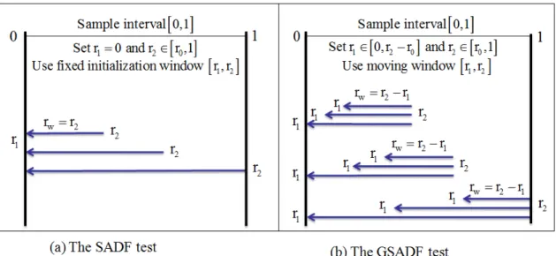
The SADF test estimates the ADF model repeatedly on a forward expanding sample sequence and conducts a hypothesis test based on the sup value of the corresponding ADF statistic sequence. The window size  expands from 0 to 1 where 0 is the smallest sample window

(selected to ensure estimation efficiency) and1 is the largest sample window (the total sample size). The starting point 1 of the sample sequence is fixed at 0 so the ending point of each

sample2 is equal to, changing from0 to1. The ADF statistic for a sample that runs from0

to2 is denoted by02. The SADF statistic is defined assup2∈[01] 2

0 and is denoted

by (0).

The SADF test and other right-sided unit root tests are not the only method of detecting explosive behavior. An alternative approach is the two-regime Markov-switching unit root test of Hall, Psaradakis and Sola (1999). While this procedure offers some appealing features like regime probability estimation, recent simulation work by Shi (2011) reveals that the Markov switching model is susceptible to false detection or spurious explosiveness. In addition, when allowance is made for a regime-dependent error variance as in Funke, Hall and Sola (1994) and van Norden and Vigfusson (1998), filtering algorithms can find it difficult to distinguish periods which may appear spuriously explosive due to high variance and periods when there is genuine explosive behavior. Furthermore, the bootstrapping procedure embedded in the Markov switching unit root test is computationally burdensome as Psaradakis, Sola and Spagnolo (2001) pointed out. These pitfalls make the Markov switching unit root test a difficult and somewhat unreliable tool offinancial surveillance.

Other econometric approaches may be adapted to use the same recursive feature of the SADF test, such as the modified Bhargava statistic (Bhargava, 1986), the modified Busetti-Taylor statistic (Busetti and Busetti-Taylor, 2004), and the modified Kim statistic (Kim, 2000). These tests are considered in Homm and Breitung (2011) for bubble detection and all share the spirit of the SADF test of PWY. That is, the statistic is calculated recursively and then the sup functional of the recursive statistics is calculated for testing. Since all these tests are similar in character to the SADF test and since Homm and Breitung (2011) found in their simulations that the PWY test was the most powerful in detecting multiple bubbles, we focus attention in

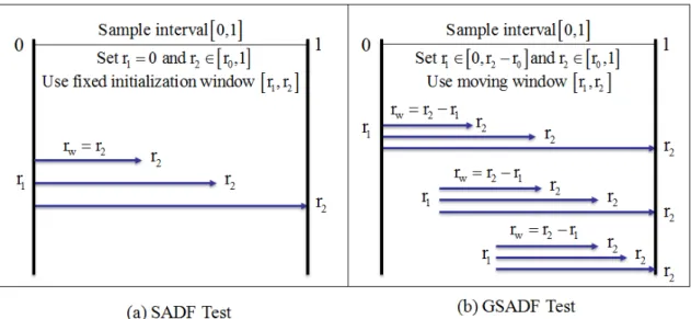
Figure 1: The sample sequences and window widths of the SADF test and the GSADF test

this paper on the SADF test. However, in our empirical application we provide comparative results with the CUSUM procedure in view of its good overall performance in the Homm and Breitung simulations.

The GSADF test deployed in the current paper continues the idea of repeatedly running the ADF test regression (4) on a sample sequence. However, the sample sequence is broader than that of the SADF test. Besides varying the end point of the regression2 from 0to1, the

GSADF test allows the starting points 1 to change within a feasible range, which is from0 to 2−0. Figure 1 illustrates the sample sequences of the SADF test and the GSADF test. We

define the GSADF statistic to be the largest ADF statistic over the feasible ranges of 1 and 2, and we denote this statistic by (0)That is,

(0) = sup 2∈[01] 1∈[02−0] © 2 1 ª 

Proposition 1 When the regression model includes an intercept and the null hypothesis is a random walk with an asymptotically negligible drift (i.e. − with   12 and constant ),

the limit distribution of the GSADF test statistic is: sup 2∈[01] 1∈[02−0] ⎧ ⎪ ⎪ ⎪ ⎨ ⎪ ⎪ ⎪ ⎩ 1 2 h (2)2−(1)2− i −R2 1 ()[(2)−(1)] 12 ½ R2 1 () 2 ₋hR2 1 () i2¾12 ⎫ ⎪ ⎪ ⎪ ⎬ ⎪ ⎪ ⎪ ⎭  (5)

where =2−1 and  is a standard Wiener process.

The proof of Proposition 1 is similar to that of PWY and is given in the technical supplement to the paper (Phillips, Shi and Yu, 2011b). The limit distribution of the GSADF statistic is identical to the case when the regression model includes an intercept and the null hypothesis is a random walk without drift. The usual limit distribution of the ADF statistic is a special case of equation (5) with1 = 0 and 2 = = 1 while the limit distribution of the SADF statistic

is a further special case of equation (5) with 1 = 0 and 2 = ∈[01](see Phillips, Shi and

Yu, 2011a).

Similar to the SADF statistic, the asymptotic GSADF distribution depends on the smallest window size0. In practice,0 needs to be chosen according to the total number of observations If is small,0 needs to be large enough to ensure there are enough observations for adequate

initial estimation. If is large, 0 can be set to be a smaller number so that the test does not

miss any opportunity to detect an early explosive episode. In our empirical application we use

0 = 361680corresponding to around2%of the data.

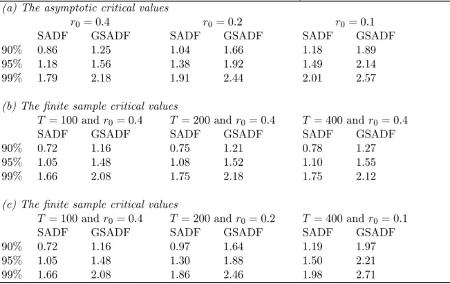
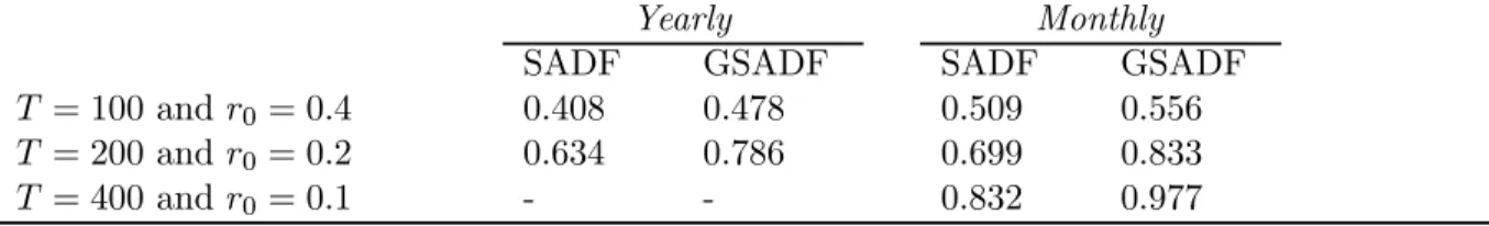
Critical values of the SADF and GSADF statistics are displayed in Table 1. The asymptotic critical values are obtained by numerical simulations, where the Wiener process is approximated by partial sums of 2000independent (01) variates and the number of replications is 2000. The finite sample critical values are obtained from 5000 Monte Carlo replications. The lag order is set to zero. The parameters, and , in the null hypothesis are set to unity.7

We observe the following phenomena. First, as the minimum window size 0 decreases,

critical values of the test statistic (including the SADF statistic and the GSADF statistic) increase. For instance, when 0 decreases from 04 to01, the 95% asymptotic critical value of

7

From Phillips, Shi and Yu (2011a), we know that when= 1and 12, thefinite sample distribution of the SADF statistic is almost invariant to the value of.

Table 1: Critical values of the SADF and GSADF tests against an explosive alternative (a) The asymptotic critical values

0 = 04 0 = 02 0 = 01

SADF GSADF SADF GSADF SADF GSADF

90% 0.86 1.25 1.04 1.66 1.18 1.89

95% 1.18 1.56 1.38 1.92 1.49 2.14

99% 1.79 2.18 1.91 2.44 2.01 2.57

(b) The finite sample critical values

 = 100 and0= 04  = 200 and0= 04  = 400and 0= 04

SADF GSADF SADF GSADF SADF GSADF

90% 0.72 1.16 0.75 1.21 0.78 1.27

95% 1.05 1.48 1.08 1.52 1.10 1.55

99% 1.66 2.08 1.75 2.18 1.75 2.12

(c) The finite sample critical values

 = 100 and0= 04  = 200 and0= 02  = 400and 0= 01

SADF GSADF SADF GSADF SADF GSADF

90% 0.72 1.16 0.97 1.64 1.19 1.97

95% 1.05 1.48 1.30 1.88 1.50 2.21

99% 1.66 2.08 1.86 2.46 1.98 2.71

Note: the asymptotic critical values are obtained by numerical simulations with 2,000 iterations. The Wiener process is approximated by partial sums of(01)with2000steps. The finite sample critical values are obtained from the5000Monte Carlo simulations. The parameters,and, are set to unity.

the GSADF statistic rises from 156 to214 and the95%finite sample critical value of the test statistic with sample size400increases from148to221. Second, for a given0, thefinite sample

critical values of the test statistic are almost invariant. Third, critical values for the GSADF statistic are larger than those of the SADF statistic. As a case in point, when  = 400 and

0 = 01, the95% critical value of the GSADF statistic is221while that of the SADF statistic

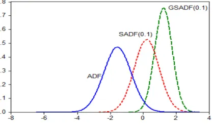
is150. Figure 2 shows the asymptotic distribution of the,(01)and(01) statistics. The distributions move sequentially to the right and have greater concentration in the order,(01)and (01).

Figure 2: Asymptotic distributions of the ADF and supADF statistics (0 = 01)

3

Simulations

3.1

Generating the test sample

We first simulate an asset price series based on the Lucas asset pricing model and the Evans (1991) bubble model. The simulated asset prices consist of a market fundamental component

_, which combines a random walk dividend process and equation (1) with = 0and = 0 for all to obtain8

=+₋1+  ∼ ¡ 0 2_¢ (6) _ =  (1₋)2 +  1₋ (7)

and the Evans bubble component

+1=−1+1 if   (8)

8

An alternative data generating process, which assumes that the logarithmic dividend is a random walk with drift, is as follows: ln=+ ln−1+ ∼  0 2  _ = exp  +1 2 2   1−exp+12 2  

+1=

h

+ ()−1+1(−)

i

+1 if ≥  (9)

This series has the submartingale property _E(+1) = (1 +) Parameter  is the drift

of the dividend process, 2_ is the variance of the dividend,  is a discount factor with −1 = 1+ 1and = exp ¡ −22 ¢ with∼  ¡

0 2¢. The quantity is the re-initializing value after the bubble collapse. The series  follows a Bernoulli process which takes the value 1with probability and0with probability1₋. Equations (8) - (9) state that a bubble grows explosively at rate−1 when its size is less thanwhile if the size is greater than , the bubble grows at a faster rate ()−1 but with a 1₋ probability of collapsing. The asset price is the sum of the market fundamental and the bubble component, namely=_+, where 0 controls the relative magnitudes of these two components.

The parameter settings used by Evans (1991) are displayed in the top line of Table 2 and labeled yearly. The parameter values for  and 2_ were originally obtained by West (1988), by matching the sample mean and sample variance offirst differenced real S&P 500 stock price index dividends from 1871 to 1980. The value for the discount factor  is equivalent to a 5% yearly interest rate.

Table 2: Parameter settings

 2_ 0   0    

Yearly 0.0373 0.1574 1.3 0.952 1 0.50 0.85 0.50 0.05 20 Monthly 0.0024 0.0010 1.0 0.985 1 0.50 0.85 0.50 0.05 50

Due to the availability of higher frequency data, we apply the SADF test and the GSADF test to monthly data. The parameters  and 2_ are set to correspond to the sample mean and sample variance of the first differenced monthly real S&P 500 stock price index dividend described in the application section below, so that the settings are in accordance with our empirical application. The discount valueequals0985(we allowto vary from 0.975 to 0.999 in the size and power comparisons section). The new setting is labeledmonthly in Table 2.

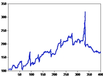
Figure 3 depicts one realization of the data generating process with the monthly parameter settings. As we observe in this graph, there are several obvious collapsing episodes of different magnitudes within this particular sample trajectory.

Figure 3: Simulated time series of=+ using the Evans collapsing bubble model with

sample size 400and monthly parameter settings.

3.2

Implementation of the new test

We first implement the SADF test on the whole sample range. We repeat the test on a sub-sample which contains fewer collapsing episodes to illustrate the instability of the SADF test. Furthermore, we conduct the test on the same simulated data series (over the whole sample range) to show the advantage of the GSADF test.

The lag orderis set to zero for all tests in this paper.9 The smallest window size considered in the SADF test for the whole sample contains 40observations (0 = 01). The SADF statistic

for the simulated data series is 071, which is smaller than the10% finite sample critical value 119(see Table 1). Therefore, we conclude that there are no bubbles in this sample. Now suppose that the SADF test starts from the 201 _{observation, and the smallest regression window also}

contains40 observations (0 = 02). The SADF statistic obtained from this sample is 139 and

it is greater than 130 (Table 1). In this case, we reject the null hypothesis of no bubble at the 5%significance level.

9_{In PWY, the lag order was determined by significance testing, as in Campbell and Perron (1991). However,} we demonstrate in the size and power comparison section below that this lag selection criteria results in significant size distortion and reduces the power of both the SADF and GSADF tests.

Evidently the SADF test fails tofind bubbles when the whole sample is utilized, whereas by re-selecting the starting point of the sample to exclude some of the collapse episodes, it succeeds in finding evidence of bubbles. Each of the above experiments can be viewed as special cases of the GSADF test in which the sample starting points are fixed. In the first experiment, the sample starting point of the GSADF test 1 is set to 0. The sample starting point 1 of the

second experiment isfixed at0502. The conflicting results obtained from these two experiments demonstrates the importance of using variable starting points, as is done in the GSADF test.

We then apply the GSADF test to the simulated asset prices. The GSADF statistic of the simulated data is859, which is substantially greater than the1%finite sample critical value271 (Table 1). Thus, the GSADF testfinds strong evidence of bubbles. Compared to the SADF test, the GSADF identifies bubbles without re-selecting the sample starting point, giving an obvious improvement that is particularly useful in empirical applications.10

3.3

Size and Power Comparisons

This section compares the sizes and powers of the SADF and GSADF tests. The data generating process for the size comparison is the null hypothesis in equation (3) with  =  = 1. We calculate size based on the asymptotic critical values displayed in Table 1. The nominal size is 5%. The number of replications is5000. We observe from Table 3 that the size distortion of the GSADF test is smaller than that of the SADF test. For example, when  = 400 and 0 = 01,

the size distortion of the GSADF test is 09%whereas that of the SADF test is16%.11

Powers in Table 4 and 5 are calculated with the 95% quantiles of the finite sample distribu-tions (Table 1), and the number of iteradistribu-tions for the calculation is5000. The smallest window size for both the SADF test and the GSADF test has 40 observations. The data generating process of the power comparison is the periodically collapsing explosive process, equations (6) 1 0_{We observe similar phenomena from the alternative data generating process where the logarithmic dividend} is a random walk with drift. Parameters in the alternative data generating process (monthly) are set as follows: 0 = 05 = 1 = 085 = 05 = 0985  = 005 = 0001ln0= 1,2ln= 00001, and=+ 500.

1 1_{Suppose the lag order is determined by significance testing as in Campbell and Perron (1991) with a maximum} lag order of12. When= 400and0= 01, the sizes of the SADF test and the GSADF test are0130and0790

(the nominal size is5%), indicating size distortion in both tests and a particularly large size distortion for the GSADF test.

Table 3: Sizes of the SADF and GSADF tests with asymptotic critical values. The data gener-ating process is equation (3) with == 1. The nominal size is 5%.

 = 100  = 200  = 400

0= 04 0 = 04 0 = 02 0= 04 0 = 01

SADF 0.043 0.040 0.038 0.041 0.034

GSADF 0.048 0.041 0.044 0.045 0.059

Note: size calculations are based on 5000 replications..

- (9). For comparison with the literature, we first set the parameters in the DGP as in Evans (1991) with sample sizes of 100 and 200. From the left panel of Table 4 (labeled yearly), the power of the GSADF test is7%and152%higher than those of the SADF test when the sample size is100and 200.12

Table 4: Powers of the SADF and GSADF tests. The data generating process is equation (6)-(9). Yearly Monthly

SADF GSADF SADF GSADF

 = 100 and0= 04 0.408 0.478 0.509 0.556  = 200 and0= 02 0.634 0.786 0.699 0.833

 = 400 and0= 01 - - 0.832 0.977

Note: power calculations are based on 5000 replications.

Table 4 also displays powers of the SADF and GSADF tests under the DGP with monthly parameter settings and sample sizes 100, 200 and 400. From the right panel of the table, when the sample size = 400, the GSADF test raises test power from832%to977%, giving a145% improvement. The power improvement of the GSADF test is 47% when  = 100 and 134% when  = 200. For any given bubble collapsing probability  in the Evans model, the sample period is more likely to include multiple collapsing episodes the larger the sample size. Hence, the advantages of the GSADF test are more evident for large.

In Table 5, we compare powers of the SADF and GSADF tests with the discount factor 

varying from 0975 to 0990, under the DGP with the monthly parameter settings. First, due 1 2_{Suppose the lag order is determined by significance testing as in Campbell and Perron (1991) with a maximum} lag order of12. When  = 200and 0 = 02, the powers of the SADF test and the GSADF test are0565and

to the fact that the rate of bubble expansion is inversely related to the discount factor, powers of both SADF test and GSADF tests are expected to decrease as  increases. The power of the SADF (GSADF) test declines from845% to769%(from 993%to910%) as the discount factor rises from0975to0990(see Table 5). Second, we observe from Table 5 that the GSADF test has greater discriminatory power for detecting bubbles than the SADF test. The power improvement is 148%,148%,145%and 141%for=_{0975098009850990_}.

Table 5: Powers of the SADF and GSADF tests. The data generating process is equations (6)-(9) with themonthly parameter settings and sample size 400 (0= 01).

 0.975 0.980 0.985 0.990

SADF 0.845 0.840 0.832 0.769

GSADF 0.993 0.988 0.977 0.910

Note: power calculations are based on 5000 replications.

4

Date-stamping Strategies

Suppose that one is interested in knowing whether any particular observation, such as the point b 2c, belongs to a bubble phase in the trajectory. PWY suggest conducting a right-tailed ADF

test recursively using information up to this observation (i.e. _b 2c =

©

1 2· · · _b 2c

ª

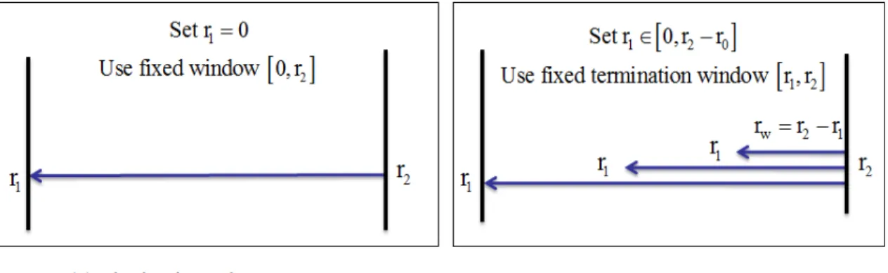
). Since it is possible that _{b 2c} includes one or more collapsing bubble episodes, the ADF test, like the cointegration-based test for bubbles, may result in findingpseudo stationary behavior. We therefore recommend performing abackward sup ADF teston_b 2cto improve identification accuracy.

The backward SADF test performs a sup ADF test on a backward expanding sample se-quence, where the ending points of the samples are fixed at 2 and the starting point varies

from 0 to 2−0. Suppose we label the ADF statistic for each regression using its starting

point 1 and ending point 2 to obtain12. The corresponding ADF statistic sequence is

©

2 1

ª

1∈[02−0]. The backward SADF statistic is defined as the sup value of the ADF statistic sequence, denoted by

2(0) = sup 1∈[02−0] © 2 1 ª 

Figure 4: The sample sequences of the backward ADF test and the backward SADF test

The backward ADF test is a special case of the backward sup ADF test with 1 = 0. We

denote the backward ADF statistic by 2. Figure 4 illustrates the difference between the backward ADF test and the backward SADF test. PWY propose comparing2 with the (right-tail) critical values of the standard ADF statistic to identify explosiveness at observation b 2c. The feasible range of 2 runs from 0 to 1. The origination date of a bubble b c

is calculated as the first chronological observation whose backward ADF statistic exceeds the critical value. We denote the calculated origination date by _bˆ_c. The estimated termination date of a bubble_bˆcis thefirst chronological observation afterbˆc+log ()whose backward

ADF statistic goes below the critical value. PWY impose a condition that for a bubble to exist its duration must exceed log (). This requirement helps to exclude short lived blips in the

fitted autoregressive coefficient. The dating estimates are then

ˆ  = inf 2∈[01] n 2 :2    2 o and ˆ = inf 2∈[ˆ+log()1] n 2 :2    2 o  (10) where 

2 is the 100% critical value of the backward ADF statistic based on b 2c

obser-vations. The significance level_ depends on the sample size  and we assume that_{ →}0 as

 _{→ ∞}.

the explosiveness of observation_b 2cbased on the backward sup ADF statistic,2(0). We define the origination date of a bubble as the first observation whose backward sup ADF statistic exceeds the critical value of the backward sup ADF statistic. The termination date of a bubble is calculated as thefirst observation after_bˆc+log ()whose backward sup ADF

statistic falls below the critical value of the backward sup ADF statistic. Here it is assumed that the duration of the bubble exceedslog (), where is a frequency dependent parameter.13 The (fractional) origination and termination points of a bubble (i.e.  and ) are calculated according to the followingfirst crossing time equations:

ˆ = inf 2∈[01] n 2 :2(0)   2 o  (11) ˆ  = inf 2∈[ˆ+log()1] n 2:2(0)   2 o  (12) where

2 is the100%critical value of the sup ADF statistic based onb 2c observations.

Analogously, the significance level _ depends on the sample size  and it goes to zero as the sample size approaches infinity.

In addition, the SADF test can be viewed as a repeated implementation of the backward ADF test for each 2 ∈ [01]. The GSADF test is equivalent to a test which implements the

backward sup ADF test repeatedly for each2 ∈[01] and makes inferences based on the sup

value of the backward sup ADF statistic sequence, _{2(0)}2∈[01]. Hence, the SADF and GSADF statistics can respectively be rewritten as

(0) = sup 2∈[01] {2}, (0) = sup 2∈[01] {2(0)}

Thus, the PWY date-stamping strategy corresponds to the SADF test and the new strategy corresponds to the GSADF test. The essential features of the two tests are shown in stylized form in the diagrams of Figure 5.

1 3_{For instance, one might wish to impose a minimal condition that to be classified as a bubble its duration} should exceed a certain period such as one year (which is inevitably arbitrary). Then, when the sample size is30 years (360months),is07for yearly data and5for monthly data.

Figure 5: An alternative illustration of the sample sequences and window widths of the SADF test and the GSADF test

4.1

The null hypothesis: no bubbles

In order to derive the consistency properties of these date-stamping strategies, we first need to obtain the asymptotic distributions of the ADF statistic and the SADF statistic with_b 2c

observations under the null hypothesis (3). We know that the backward ADF test with obser-vation _b 2c is a special case of the GSADF test with 1 = 0and a fixed 2 and the backward

sup ADF test is a special case of the GSADF test with a fixed2 and 1=2−. Therefore,

based on equation (5), we can derive the asymptotic distributions of these two statistics, namely

2() := 1 22 h (2)2−2 i −R2 0 ()(2) 1₂2 n 2 R2 0 () 2 ₋£R2 0 () ¤2o12 0 2 () := sup 1∈[02−0] =2−1 ⎧ ⎪ ⎪ ⎪ ⎨ ⎪ ⎪ ⎪ ⎩ 1 2 h (2)2−(1)2− i −R2 1 ()[(2)−(1)] 12 ½ R2 1 () 2 ₋hR2 1 () i2¾12 ⎫ ⎪ ⎪ ⎪ ⎬ ⎪ ⎪ ⎪ ⎭  We, therefore, define

2 as the100 (1−) %quantile of2()and  2 as the100 (1−) % quantile of0 2 (). We know that  2 → ∞and   2 → ∞ as →0.

Given

2 → ∞and 

2 → ∞, under the null hypothesis of no bubbles, the probabilities of (falsely) detecting the origination of bubble expansion and the termination of bubble collapse using the backward ADF statistic and the backward sup ADF statistic tend to zero, so that both Pr_{ˆ ∈[01]}→0and Pr{ˆ ∈[01]}→0.

4.2

The alternative hypothesis: a single bubble

Consider the data generating process of Phillips and Yu (2009)

=−11{  }+−11{ ≤≤} + ⎛ ⎝  X =+1 +∗ ⎞ ⎠1_{  }+1{≤} (13)

where  = 1 +− with   0 and ∈ (01)  

∼ ¡0 2¢_{, }∗

 = +∗ with ∗ = (1),  = b c is the origination of bubble expansion and  = b c is the termination

of bubble collapse. The pre-bubble period 0 = [1 ) is assumed to be a pure random walk

process. The bubble expansion period= [ ]is a mildly explosive process with expansion

rate . The process then collapses to _∗_, which equals  plus a small perturbation, and continues its pure random walk path in the period 1= ( ].

Notice that there is only one bubble episode in the data generating process (13). Under this mechanism we have the following consistency results, whose proofs are collected in Appendix A. Theorem 1 Supposeˆ andˆ are obtained from the backward DF test based on the t statistic, (10). Given an alternative hypothesis of mildly explosive behavior in model (13), if

1  2 +  2 12 →0 (14) we have ˆ  → and ˆ  → as  → ∞.

Theorem 2 Suppose ˆ and ˆ are obtained from the backward sup DF test based on the t

statistic, (11) - (12). Given an alternative hypothesis of mildly explosive behavior in model (13), if 1  2 +  2 12 →0 (15)

we have ˆ _→  and ˆ _→  as  _{→ ∞}.

These results show that both strategies consistently estimate the origination and termination points when there is only a single bubble episode in the sample period. Suppose

2 =( ₎

and 

2 = (

_{). The regularity condition (14) in Theorem 1 implies that the order of} magnitude () of 

2 needs to be greater than 0 and smaller than 12, namely  ∈ (012). Theorem 2 requires the order of magnitude (_) of

2 to be greater than0 and smaller than

12 to obtain the consistency of ˆ and ˆ.

4.3

The alternative hypothesis: two bubbles

Consider a data generating process with two bubble episodes:

=₋11{∈0}+−11{∈1∪2}+ ⎛ ⎝  X =1+1 +∗1 ⎞ ⎠1_{_∈1} + ⎛ ⎝  X =2+1 +∗2 ⎞ ⎠1_{_∈2}+1{∈0∪1∪2} (16) where 0 = [1 1) 1 = [1 1] 1 = (1 2) 2 = [2 2] and 2 = (2 ]. 1 = b 1c,1 =b 1care the origination and termination dates of thefirst bubble,2=b 2c, 2 =b 2c are the origination and termination dates of the second bubble and  is the last

observation of the sample. After the collapse of the first bubble, continues its pure random

walk path until2−1and starts another expansion process at2. The expansion process lasts

until 2 and collapses to a value of ∗2. It then continues its pure random walk path until the end of the sample period . We assume that the expansion duration of the first bubble is longer than that of the second bubble, namely1 −1 2 −2.

The date-stamping strategy of PWY suggests calculating 1, 1, 2 and 2 from the

following equations (based on the ADF statistic): ˆ 1= inf 2∈[01] n 2:2    2 o and ˆ1 = inf 2∈[ˆ1+log()1] n 2 :2    2 o  (17)

ˆ 2= inf 2∈[ˆ11] n 2 :2    2 o and ˆ2 = inf 2∈[ˆ2+log()1] n 2:2    2 o  (18) where the duration of the bubble periods is restricted to be longer than log ().

The new strategy recommends using the backward sup ADF test and calculating the origi-nation and termiorigi-nation points according to the following equations:

ˆ 1= inf 2∈[01] n 2 :2(0)  _ 2 o  (19) ˆ 1 = inf 2∈[ˆ1+log()1] n 2:2(0)   2 o  (20) ˆ 2= inf 2∈[ˆ11] n 2 :2(0)   2 o  (21) ˆ 2 = inf 2∈[ˆ2+log()1] n 2:2(0)   2 o  (22)

An alternative implementation of the PWY procedure is to use that procedure sequentially, namely detect one bubble at a time. The dating criteria for the first bubble remains the same (i.e. equation (17)). Conditional on thefirst bubble having been found and terminated atˆ1,

the following dating criteria is used for a second bubble: ˆ 2= inf 2∈(ˆ1+1] n 2 :ˆ1 2    2 o and ˆ2 = inf 2∈[ˆ2+log()1] n 2:ˆ1 2    2 o  (23) where ˆ12 is the ADF statistic calculated over (ˆ1 2]. Note that we need a few obser-vations to initialize the procedure (i.e. 2 ∈(ˆ1+1]for some 0).14

We have the following asymptotic results for these dating estimates. Proofs of the theorems are given in Appendix B.

Theorem 3 Supposeˆ1,ˆ1, ˆ2 andˆ2 are obtained from the backward DF test based on the

t statistic, (17) - (18). Given an alternative hypothesis of mildly explosive behavior of model (16) with1 −1  2 −2, if 1  2 +  2 12 →0 1 4_{For example,}

we have ˆ1 

→ 1 and ˆ1 

→ 1 as  → ∞; and ˆ2 and ˆ2 are not consistent estimators of 2 and 2.

Theorem 4 Supposeˆ1,ˆ1, ˆ2 and ˆ2 are obtained from the backward sup DF test based on

the t statistic, (19) - (22). Given an alternative hypothesis of mildly explosive behavior of model (16) with1 −1  2 −2, if 1  2 + _ 2 12 →0 we have ˆ1  →1 ˆ1  →1, ˆ2  →2 andˆ2  →2 as → ∞.

Theorem 5 Supposeˆ1,ˆ1, ˆ2 andˆ2 are obtained from the backward DF test based on the

t statistic, (17) and (23). Given an alternative hypothesis of mildly explosive behavior of model (16) with1 −1  2 −2, if 1  2 + _ 2 12 →0 we have ˆ1  →1, ˆ1  →1, ˆ2  →2 and ˆ2  →2 as  → ∞.

A restatement of Theorem 3 is useful. Suppose the sample period includes two bubble episodes and the duration of the first bubble is longer than the second. The strategy of PWY (corresponding to the SADF test) can consistently estimate the origination and termination of thefirst bubble but does not consistently estimate those of the second bubble. In contrast, The-orem 4 and TheThe-orem 5 say that the new date-stamping strategy (corresponding to the GSADF test) and the alternative implementation of the PWY strategy can calculate the origination and termination of both bubbles consistently in this scenario.

We also analyze the consistency properties of these two date-stamping strategies when there are two bubbles and the duration of the first bubble is shorter than the second bubble. Under this circumstance, the strategy of PWY cannot estimate the origination date of the second bubble consistently15, whereas the new strategy can consistently estimate the origination and termination dates of the two bubbles.16

1 5

It can consistently estimate the origination date of thefirst bubble and the termination dates of both bubbles. 1 6_{The proof is similar to the proofs of Theorems 3, 4 and 5 (Appendix B) and is omitted for brevity.}

Theorem 3, 4 and 5 can be extended to a multiple bubbles scenario. Suppose there are 

bubbles ( 2). If the duration of the bubble is longer than that of the  bubble, where

 _∈{12_{· · ·} _} and  , then, the PWY strategy can consistently estimate the origination and termination dates of the_{bubble but not those associated with the}_{bubble. In contrast,}

the new strategy and the alternative implementation of the PWY strategy can estimate dates associated with both bubbles consistently.

5

Empirical Application

We consider a long historical time series in which many crisis events are known to have occurred. The data comprise the real S&P 500 stock price index and the real S&P 500 stock price index dividend, both obtained from Robert Shiller’s website. The data are sampled monthly over the period from January 1871 to December 2010, constituting 1,680 observations and are plotted in Figure 6 by the solid (blue) line.

We first apply the SADF test and the GSADF test to the price-dividend ratio. Table 6 presents critical values for these two tests and these were obtained from Monte Carlo simulation with2000replications (sample size1680). In performing the ADF regressions and calculating critical values, the smallest window comprised 36 observations. From Table 6, the SADF and GSADF statistics for the full data series are 330 and 421. Both exceed their respective 1% right-tail critical values (i.e. 330217 and421331), giving strong evidence that the S&P 500 price-dividend ratio had explosive subperiods. We conclude from both tests that there is evidence of bubbles in the S&P 500 stock market data.

Table 6: The SADF test and the GSADF test of the S&P 500 stock market

SADF GSADF

S&P500 Price-Dividend Ratio 3.30 4.21

Finite sample critical values

90% 1.45 2.55

95% 1.70 2.80

99% 2.17 3.31

Note: Critical values of both tests are obtained from Monte Carlo simulation with2000 replications ( sample size 1,680). The smallest window has 36 observations.

To locate specific bubble periods, we compare the backward SADF statistic sequence with the95% SADF critical value sequence, which were obtained from Monte Carlo simulation with 2000 replications. The top panel of Figure 6 displays results for the date-stamping strategy over the period from January 1871 to December 1949 and the bottom panel displays results over the rest of the sample period. The identified exuberance and collapse periods includethe great crash episode (1929M01-M09), the postwar boom in 1954 (1954M12-1955M12), black Monday in October 1987 (1987M02-M09), the dot-com bubble (1995M12-2001M06) and the subprime mortgage crisis (2008M10-2009M03). The durations of those episodes are greater than or equal to half a year.17 This strategy also identifies several episodes of crisis or explosiveness whose durations are shorter than half a year, for instance, the explosive recovery phase following the panic of 1873 (1879M10-1880M02), the banking panic of 1907 (1907M10-M11) and the 1974 stock market crash (1974M09).

Notice that the new date-stamping strategy not only locates the explosive expansion periods but also identifies collapse episodes. Market collapses have occurred in the past when bubbles in other markets crashed and the collapse spread to the S&P 500 as, for instance, in the dot-com bubble collapse and the subprime mortgage crisis.

Figure 7 plots the ADF statistic sequence against the 95% ADF critical value sequence. We can see that the strategy of PWY (based on the SADF test) identifies only two explosive periods — the recovery phase of the panic of 1873 (1879M10-1880M04) andthe dot-com bubble (1997M07-2001M08).18

The PWY strategy is called FLUC monitoring in the Homm and Breitung (2011) simula-tion study, with some variasimula-tions in the implementasimula-tion procedure. Their simulasimula-tion findings show that FLUC monitoring has higher power than other procedures in detecting periodically collapsing bubbles of the Evans (1991) type, the closest rival being the CUSUM procedure. For comparison, we therefore applied the CUSUM monitoring procedure to the S&P 500 price-1 7_{If bubble duration is restricted to be longer than three months, the strategy identifies one more bubble episode,} namely the explosive recovery phase followingthe panic of 1873 (1879M10-1880M02).

1 8

If we restrict the duration of a bubble to be longer than twelve months, the new dating strategy identifies two bubble episodes: the postwar boom in 1954 (1954M12-1955M12) andthe dot-com bubble(1995M12-2001M06). In that case the strategy of PWY only identifiesthe dot-com bubble (1997M07-2001M08).

dividend ratio (ex post). The CUSUM detector is denoted by_₀ and defined as _₀ = 1 ˆ  b_X c =b 0c+1 ∆ withˆ2 = (b c−1)− 1 b_X c =1 (∆ −ˆ)2

where _b 0c is the training sample,19 b c is the monitoring observation, ˆ is the mean of

©

∆1 ∆_b c

ª

, and   0. Under the null hypothesis of a pure random walk, it has the

following asymptotic property (see Chu, Stinchcombe and White (1996)) lim →∞ n _₀  p_b _c for some_∈(01] o ≤ 1₂exp (₋2) where = p + log (0).20

The CUSUM detector is applied to detrended data (i.e. to the residuals from the regression of

 on a constant and a linear time trend). To be consistent with the SADF and GSADF dating strategies, we choose a training sample of 36 months. Figure 8 plots the CUSUM detector sequence against the 95% critical value sequence. The critical value sequence is obtained from Monte Carlo simulation (through application of the CUSUM detector to data simulated from a pure random walk) with 2,000 replications.

As it is evident in Figure 8, the CUSUM test identifies four bubble episodes for periods before 1900. For the post-1900 sample, the procedure detects only the great crash and the dot-com bubble episodes. It does not provide any warning alert or acknowledgment of black Monday in October 1987 and the subprime mortgage crisis in 2008, among other episodes identified by the GSADF dating strategy. So CUSUM monitoring may be regarded as a relatively conservative surveillance device.21

1 9

It is assumed that there is no structural break in the training sample. 2 0_{When the significance level = 005, for instance,}

005 equals46.

2 1

The conservative nature of the test arises from the fact the residual variance estimateˆ (based on the data 

1  b c



) can be quite large when the sample includes periodically collapsing bubble episodes, which may have less impact on the numerator due to collapses, thereby reducing the size of the CUSUM detector.

Figure 8: Date-stamping bubble periods in the S&P 500 price-dividend ratio: the CUSUM monitoring procedure.

6

Conclusion

The GSADF test is a rolling window right-sided ADF unit root test with a double-sup window selection criteria.22 As distinct from the SADF test of PWY, we select a window size using the double-sup criteria and implement the ADF test repeatedly on a sequence of samples, which moves the window frame gradually toward the end of the sample. Experimenting on simulated asset prices reveals one of the shortcomings of the SADF test - its reduced capacity to find and locate bubbles when there are multiple collapsing episodes within the sample range. The GSADF test surmounts this problem and our simulationfindings demonstrate that the GSADF test significantly improves discriminatory power in detecting multiple bubbles.

The date-stamping strategy of PWY and the new date-stamping strategy are shown to have quite different behavior under the alternative of multiple bubbles. In particular, when the sample period includes two bubbles and the duration of the first bubble is longer than the second, the strategy of PWY fails to consistently estimate the timing of the second bubble while the new strategy consistently estimates and dates both bubbles.

We apply both SADF and GSADF tests, along with their date-stamping algorithms and the alternative CUSUM monitoring procedure considered in Homm and Breitung (2011), to the S&P 500 price-dividend ratio from January 1871 to December 2010. All three tests find confirmatory evidence of multiple bubble existence. The price-dividend ratio over this historical period contains many individual peaks and troughs, a trajectory that is similar to the multiple bubble scenario for which the PWY date-stamping strategy was found to be inconsistent. The empirical test results confirm the greater discriminatory power of the GSADF strategy found in the simulations and evidenced in the asymptotic theory. The new date-stamping strategy identifies all the well known historical episodes of banking crises and financial bubbles over this long period, whereas both SADF and CUSUM procedures seem more conservative and locate fewer episodes of exuberance and collapse.

2 2_{First, we calculate the sup value of the ADF statistic over the feasible ranges of the window starting points} for afixed window size. Then, we calculate the sup value of the SADF statistic over the feasible range of window sizes.

7

References

Ahamed, L., 2009,Lords of Finance: The Bankers Who Broke the World, Penguin Press, New York.

Bhargava, A. 1986, On the theory of testing for unit roots in observed time series, Review of Economic Studies, 53, 369—384.

Busetti, F., and A. M. R. Taylor, 2004, Tests of stationarity against a change in persistence, Journal of Econometrics, 123, 33—66.

Campbell, J.Y., and Perron, P., 1991, Pitfalls and opportunities: what macroeconomists should know about unit roots. NBER Macroeconomics Annual, 6, 141—201.

Campbell, J.Y., and Shiller R.J., 1989, The dividend-price ratio and expectations of future dividends and discount factors. The Review of Financial Studies, 1, 195—228.

Charemza, W.W., and Deadman, D.F., 1995, Speculative bubbles with stochastic explosive roots: the failure of unit root testing. Journal of Empirical Finance, 2, 153—163.

Chu, C.J., Stinchcombe, M., and White, H., 1996, Monitoring structural change. Econometrica, 64:1045-1065.

Cochrane, J. H. (2005). Asset Pricing, Princeton: Princeton University Press.

Cooper, G., 2008, The Origin of Financial Crises: Central Banks, Credit Bubbles and the Efficient Market Fallacy, Vintage Books, New York.

Diba, B.T., and Grossman, H.I., 1988, Explosive rational bubbles in stock prices? The Amer-ican Economic Review, 78, 520—530.

Evans, G.W., 1991, Pitfalls in testing for explosive bubbles in asset prices. The American Economic Review, 81, 922—930.

Funke, M., Hall, S., and Sola, M., 1994, Rational bubbles during Poland’s hyperinflation: implications and empirical evidence. European Economic Review, 38, 1257—1276.

Gurkaynak, R. S., 2008, Econometric tests of asset price bubbles: taking stock. Journal of Economic Surveys, 22, 166—186.

Hall, S.G., Psaradakis, Z., and Sola M., 1999, Detecting periodically collapsing bubbles: A markov-switching unit root test. Journal of Applied Econometrics, 14, 143—154.

Hamilton, J.D., 1994, Time Series Analysis, Princeton University Press.

Homm U. and J. Breitung, 2011, Testing for Speculative Bubbles in Stock Markets: A Com-parison of Alternative Methods. Journal of Financial Econometrics, forthcoming.

Kim, J. Y. 2000, Detection of change in persistence of a linear time series, Journal of Econo-metrics, 95, 97—116.

Kindleberger, C. P., and Aliber, R. Z., 2005, Manias, Panics and Crashes; A History of Fi-nancial Crises, Hoboken, New Jersey: John Wiley and Sons, Inc.

Lee, J. and P. C. B. Phillips, 2011, Asset Pricing with Financial Bubble Risk. Yale University, Working Paper.

Pástor, Luboš, and Pietro Veronesi, 2006, Was there a Nasdaq bubble in the late 1990s? Journal of Financial Economics 81, 61—100.

Phillips, P.C.B., 1987, Time series regression with a unit root. Econometrica 55, 277-301.

Phillips, P.C.B., and Perron, P., 1988, Testing for a unit root in time series regression. Bio-metrika, 75, 335—346.

Phillips, P.C.B., and Magdalinos, T., 2007, Limit theory for moderate deviations from a unit root. Journal of Econometrics, 136, 115—130.

Phillips, P. C. B. and V. Solo, 1992, Asymptotics for Linear Processes.Annals of Statistics 20, 971—1001.

Phillips, P.C.B., Shi, S., and Yu, J., 2011a, Specification Sensitivity in Right-Tailed Unit Root Testing for Explosive Behavior. Working Paper, Sim Kee Boon Institute for Financial Economics, Singapore Management University.

Phillips, P.C.B., Shi, S., and Yu, J., 2011b, Technical Note: Testing for Multiple Bubbles. Man-uscript, available from https://sites.google.com/site/shupingshi/TN_GSADF.pdf? attredirects=0&d=1.

Phillips, P.C.B., Wu, Y., and Yu, J., 2011, Explosive behavior in the 1990s Nasdaq: When did exuberance escalate asset values? International Economic Review, 52, 201-226.

Phillips, P.C.B., and Yu, J., 2009, Limit theory for dating the origination and collapse of mildly explosive periods in time series data. Singapore Management University, Unpublished Manuscript.

Phillips, P.C.B., and Yu, J., 2011, Dating the Timeline of Financial Bubbles During the Sub-prime Crisis, Quantitative Economics, 2, 455-491.

Psaradakis, Z., Sola, M., and Spagnolo, F., 2001, A simple procedure for detecting periodically collapsing rational bubbles. Economics Letters, 24, 317—323.

Shi, S. 2011, Bubbles or volatility: the Markov-switching unit root tests. Australian National University, Working Paper.

van Norden, S. and Vigfusson, R., 1998, Avoiding the pitfalls: can regime-switching tests reliably detect bubbles? Studies in Nonlinear Dynamics & Econometrics, 3,1—22.

APPENDIX A. The date-stamping strategies (a single bubble)

Notation and useful preliminary lemmas

We define the following notation:

• The bubble period= [ ], where =b c and  =b c.

• The normal market periods 0 = [1 ) and 1 = [ + 1 ], where  =b c is the last

observation of the sample.

• The starting point of the regression1 =b 1c, the ending point of the regression 2 =

b 2c, the regression sample size=b cwith =2−1 and observation=b c.

• ()_≡()where is a Wiener process. We use the data generating process

= ⎧ ⎨ ⎩ −1+ for∈0 ₋1+ for∈ _∗_ +P_= +1 for∈1  (24)

where  = 1 +− with   0 and  ∈ (01)  

∼ ¡0 2¢ and _∗

 =  +

∗ _with

∗=(1). Under (24) we have the following lemmas.

Lemma 7.1 Under the generating process (24), (1) For _∈0, =b c∼12(). (2) For _∈, _{=b c}=−  {1 +(1)}∼ 12_−  () (3) For _∈1, =b c∼12[()−() +()]

Proof. (1) For  _∈ 0,  is a unit root process. We know that −12=b c 

→ () as

 _{→ ∞}. (2) For_∈the generating mechanism is

=₋1+=_−+ −X−1

=0

_₋

Based on Phillips and Magdalinos (2007, lemma 4.2), we know that for 1 −2 −X−1 =0 −(−)+  −  →_≡¡0 22¢

as₋→ ∞. Furthermore, we know that−12−1  →() and hence −(−)  − 12_ =−12−1+− (1−)2_−2 −X−1 =0 −(−)+  −  →()

This implies that the first term has a higher order than the second term and hence,

=_− ( 1 + P−−1 =0   − −   ) =−  {1 +(1)}∼ 12_−  () (3)For _∈1, =  X =+1 +∗ =  X =+1 + +∗ ∼ 12_[() −() +(�