Hi
-St
at
D
isc
us
si
on
Pap
er
Research Unit for Statistical
and Empirical Analysis in Social Sciences (Hi-Stat)
Hi-Stat
Institute of Economic Research Hitotsubashi University
Global COE Hi-Stat Discussion Paper Series
Research Unit for Statistical
and Empirical Analysis in Social Sciences (Hi-Stat)
March 2011
The Value of Human Capital Wealth
Julian di Giovanni
Akito Matsumoto
The Value of Human Capital Wealth
∗ Julian di GiovanniInternational Monetary Fund
Akito Matsumoto International Monetary Fund February 16, 2011
Abstract
The value of human capital wealth and its return process are important to quantify in order to study consumption behavior and portfolio allocation. This paper introduces a new approach to measure the value of an economy’s total human capital wealth. By assuming that the consumption to wealth ratio is constant, we exploit aggregate consumption data to recover total wealth, and then use household non-human capital wealth data to recover the value of human capital wealth as a residual. Using U.S. data over the period 1952–2007, we find that human capital is approximately three-quarters of total wealth in the aggregate economy, and that this ratio is remarkably stable over time. Applying our methodology to a group of OECD countries yields similar results. We estimate the cointegrating relationship between our estimated measure of human wealth and labor compensation (income) to show that our consumption-based approach estimate of human capital is linked to one based on a labor-income approach. We next calculate the returns to human capital and find them to be as high as equity returns on average but much less volatile; positively correlated with returns on real estate and consumption growth, but negatively correlated to equity returns. Finally, we show that both human capital and equity returns are predictable by human capital’s dividend to price ratio.
JEL Classifications: E21, E24, G10
Keywords: Household Wealth, Human Capital, Wealth Effect
∗
We would like to thank Catia Batista, Olivier Blanchard, Francesco Caselli, Chris Crowe, Bob Flood, Andrei Levchenko, Isabelle M´ejean, Hanno Lustig, David Romer, Ken Singleton, Luis Viceira, Ken West, and seminar participants at the Federal Reserve Board of Governors, the IMF, Notre Dame, and Vanderbilt, for helpful comments, and Mary Yang for excellent research assistance. The views expressed in this paper are those of the authors and should not be attributed to the International Monetary Fund, its Executive Board, or its management. Correspondence: International Monetary Fund, 700 19th Street NW, Washington, DC 20431, USA. E-mail (URL):JdiGiovanni@imf.org (http://julian.digiovanni.ca), AMatsumoto@imf.org
1
Introduction
The largest component of a private household’s wealth is arguably its human capital. Its rel-ative contribution to total wealth, and its return process are therefore important to quantify in order to study consumption behavior in response to different shocks (such as to wealth,
Modigliani, 1971; Lettau and Ludvigson, 2004), and portfolio allocation (Roll, 1977). In particular,Roll (1977) claims that the true ‘market portfolio’ cannot be measured without knowing human capital, and ignoring it can lead to incorrect conclusions. In response,
Campbell (1996), Jagannathan and Wang (1996), Lettau and Ludvigson (2001), Viceira
(2001) and others explicitly include labor income in the model. However, Palacios (2010) emphasizes the difference between labor income and human capital returns in a calibrated model. Therefore, households’ consumption and portfolio choices should be based on the value of their wealth, not their current income, and it is thus better to know the value of human capital rather than simply labor income in order to study household behavior.1 Providing a reliable series of the current value of human capital over time is therefore im-portant to understand consumption behavior and portfolio decisions, yet few such measures exist.
We propose to fill this gap by developing a simple methodology. Our approach relies on the assumption that consumption decisions will be based on agents’ current valuation of their human wealth and the market value of their non-human capital assets. In order to calculate total wealth using consumption data, we then rely on the stronger assumption that the consumption to wealth ratio is constant. Finally, we subtract total non-human capital assets from total wealth to recover the value of human capital wealth as a residual. The computed value of human capital can also be thought of as the expected discounted value of a stream of future labor income, just like a stock price captures the expected value of a future stream of dividends.
We apply our methodology to quarterly and annual U.S. data over the period 1952– 2007. The approach yields many interesting results. First, the human capital to total wealth share is about three-quarters on average, which roughly corresponds to the share of labor compensation in national income. This similarity is surprising given that our methodology does not rely on any compensation data. Moreover, many existing estimates of human capital wealth shares do not match this simple metric. Second, we consider the relationship between human capital and its income stream, labor compensation. We show
1
Even expected future labor income is not enough to reveal the value of human capital as the value also depends on a (time varying) discount factor.
that labor income is the only permanent component of human capital wealth, and that the labor compensation to the human capital wealth ratio (human capital’s dividend to price ratio) has predictive power for both human capital and equity returns. It is natural for this ratio to predict human capital returns, and is analogous to whatCampbell and Shiller
(1988) show in the case of the dividend to price ratio and stock returns. The predictability of equity returns arises from the robust negative correlation between human capital and equity returns that we find. Finally, these findings provide empirical support and a new interpretation for the cay approach introduced by Lettau and Ludvigson (2001).2 In our constant consumption to wealth ratio framework, we show that the deviations in cay are approximately equal to the labor compensation to human capital wealth ratio, and will thus have predictive power for equity returns.3
We next investigate the basic properties of the returns to human capital and their joint behavior with other asset returns. Human capital returns are remarkably stable over time relative to other asset returns. They are positively correlated with some classes of non-human capital asset returns such as housing, real bonds, and T-bills, but negatively correlated with domestic equity returns.4 We interpret these results as evidence that human capital, like (real) bonds or housing, provides relatively reliable cash flows. The correla-tion between human capital and housing excess returns is striking: 0.42 at the quarterly frequency, and 0.82 at the annual frequency. This finding might potentially explain why studies often find that the wealth effect for housing is larger than that of equity, as changes in housing prices might also capture changes in the value of human capital wealth, which are not captured by labor income.
We also provide calculations for a group of ten OECD countries using a recently con-structed database on household assets, and find that on average a country’s human capital to total wealth ratio is 69.8 percent. To the best of our knowledge, these are the first set of cross-country estimates of the value of human capital wealth. Our estimated levels of hu-man capital have a correlation coefficient of 0.57 with the educational attainment measures
2Thecayapproach approximates the consumption to total wealth ratio by proxying for human capital by
labor income, which requires that labor income has to be the only permanent component of human capital wealth; i.e., the two series are cointegrated (1,−1), as we find.
3Indeed,Lettau and Ludvigson’s and our results are strongest for relatively long forecast periods, akin
to whatCampbell and Shiller(1988) find for stock returns.
4Interestingly, when we use nominal returns instead of real returns, the correlation between the long bond
and human capital returns is negative, though it is positive when the sample is constrained to 1990–2007. Given that our human capital returns are negatively correlated with equity returns, this result corresponds to Campbell et al.(2009), who find that the covariance between U.S. Treasury bond returns and stock returns has moved considerably over time from positive to negative.
from the Barro and Lee(2010) dataset. We also calculate human capital returns and com-pare them to domestic equity market and housing price returns. Results are heterogeneous across countries, but the correlation with equity (housing) returns is negative (positive) for the majority of countries.
One can think of our measure as being related to the quantity of human capital in an analogous manner as the market value of physical capital, the stock price, is related to its
book value.5 Several approaches to estimate the quantity or book value of human capital
have been proposed. For example, the number of years of education or educational spending are often used to proxy for human capital.6 Labor income is also often used to estimate the value of human capital in macroeconomics and finance. Jorgenson and Fraumeni(1989) estimate shadow values of human capital using an income-based approach, where income is broadly defined as all market and non-market activity.7 This approach would be a good one if the econometrician knew the path of the future labor income stream and the discount factor as accurately as economic agents; however, given the potential uncertainty of this stream and the difficulty in valuing long-lived assets, this methodology can also be problematic.8 In addition, Jorgenson and Fraumeni’s approach calculates the book value of human capital rather than itscurrent value, which is what is relevant for rational agents making consumption decisions (based on their current information set). Nonetheless, our estimated series match up with their estimates after adjusting for non-market activity, though the correlation of the growth rates of the two series is not very high. These results are similar to the relationship between the market and book values of physical stock: they exhibit a strong long-run relationship, but differ in their short-run fluctuations.
Finally, our work complements some interesting recent research in the finance litera-ture. In a paper closely related to ours, Lustig et al. (2008) estimate the evolution of the consumption to wealth ratio. While their work also aims at understanding consumption behavior by seriously considering the role of human capital, they take the challenging ap-proach of calculating human capital wealth as the discounted sum of future labor income,
5We do not have a good measure of the quantity of human capital. Therefore, we cannot compute the
“q” of human capital in a similar manner that the investment literature computes the average Tobin’s Q for physical capital.
6By considering education spending or the cost of rearing children, early work byKendrick(1976) presents
a time series of the book value of human capital in the United States using a cost-based approach. However, using cost-based measures is problematic when studying consumption or asset allocation decisions because these proxies ignore the cash flow streams that human capital can generate.
7SeeLe et al.(2003) for a review of the cost- and income-based approaches. 8
An analogous example exists in the asset pricing literature, when the level of current stock prices cannot be well explained by dividends or earnings without also including the lagged value of stock prices.
where labor income growth and the stochastic discount factor (SDF) are estimated using a no arbitrage model with a structural vector autoregression (SVAR). This elaborate ap-proach faces several technical challenges that can potentially undermine the reliability of the estimates. First, the estimates of human capital depend on many parameters estimated by the SVAR, which in turn assumes that the economic structure underlying the estimation remains constant over the sample period (1952–2006). However, the dynamic relationships in the data may have changed over time. For example, the potential shift of the monetary policy regime during Lustig et al.’s sample period is the biggest concern, as their state vector contains the short rate, real activity, and inflation. Moreover, market frictions – particularly affecting labor income – invalidate the no-arbitrage framework, which requires frictionless asset markets.9
The assumption of a constant consumption to wealth ratio may be viewed as too re-strictive, since our methodology does not allow for any over-identifying conditions to test its validity. However, a constant consumption to wealth ratio is an implicit result of many commonly-used macroeconomic models, such as those based on log preferences or i.i.d. return processes (Samuelson, 1969; Barro,2009). Since the ratio depends only on “deep” preference parameters, it is robust to changes in economic policy over time (i.e., we avoid the
Lucas (1976) critique). Furthermore, besides it simplicity and transparency, our approach has several advantages that allow us to avoid numerous problems arising in the previous literature. First, as with stock price valuation, discounting future labor income with a con-stant discount rate will probably not provide a good estimation of human capital wealth, since the discount rate fluctuates quite a lot (Campbell, 1991). Second, getting reliable estimates of the expected labor income stream is not easy. Given the assumption that the consumption decision is based on the valuation of human capital as well as non-human cap-ital of households, our approach side-steps these difficulties by inferring the value of human capital directly. Moreover, unlike other methods used in the finance literature, our approach allows for a volatile share of human capital in total wealth. Finally, our methodology can be easily applied across countries or individuals with minimal data requirements.
The remainder of the paper is organized as follows. Section 2 provides a simple theo-retical framework to motivate the assumption of a constant consumption to wealth ratio, and discusses under what conditions it is valid. Section 3 presents the methodology for
9
Lustig and Van Nieuwerburgh(2008) also investigate the time series properties of human capital and stock market returns. They find a negative relationship between human capital and equity returns. Boyd et al.(2005) also find that unemployment news is good news for the stock market on average. We also find this negative correlation although our approach is quite different.
constructing a measure of human capital, and the data we use. Section 4presents the main results. Section 5 concludes.
2
Theoretical Motivation
Our empirical measure of human capital is derived from the assumption that the consump-tion to wealth ratio is constant. We first review condiconsump-tions for the consumpconsump-tion to wealth ratio to be constant, and then discuss the validity of our approach when the ratio is time varying. We base our discussion around the results derived byCampbell(1993) andLettau and Ludvigson (2001).10
Our estimates utilize some features of the Epstein-Zin-Weil utility where the elasticity of intertemporal substitution is unity, namely that the consumption to wealth ratio is 1−β, where β is the subjective discount factor. However, one can also simply assume that all consumers are rule of thumb consumers who spend a fixed portion of total wealth.
2.1 The Consumption to Wealth Ratio
We study an infinitely lived representative agent framework to motivate cases when the consumption to wealth ratio is constant.11 This implies that our methodology is better thought of as an approximation for aggregate human capital rather than individual levels, although our methodology can potentially be used for the individual level.12
The household maximizes the following objective function (Epstein and Zin,1989,1991;
Weil,1989): Ut= ( (1−β)Ct1−1/σ+β EtUt1+1−γ 1−1/σ 1−γ ) 1 1−1/σ , (1)
where Ct is consumption, σ is the elasticity of intertemporal substitution, and γ is the
coefficient of relative risk aversion. If σ = 1/γ, then this Epstein-Zin-Weil utility function is simplified to a time-separable constant relative risk averse utility function.
The representative household’s budget constraint is
Wt+1=Rm,t+1(Wt−Ct), (2)
10
See alsoCampbell and Mankiw(1989) for a similar derivation.
11
SeeAppendix Afor a detailed derivation of the following results.
12
Examining the individual level will be complicated by the fact that the consumption to wealth ratio may vary with age in a more realistic model. By adopting a representative agent (non-overlapping generation) model in the present paper, we are implicitly assuming that this demographic effect does not have a large impact on the aggregate estimates.
where Wt is total wealth at the beginning of period and Rm,t+1 is the gross simple return
on total wealth from timettot+ 1. Log-linearizing (2)and taking conditional expectation yields ct−wt=Et ∞ X j=1 ρj(rm,t+j−∆ct+j) + ρk 1−ρ, (3)
where lower cases denote the logarithm of the variable,ρ= 1−exp
ln WC = WW−C is the steady-state invested wealth (wealth after consumption,W −C) to total wealth (W) ratio, and k= lnρ−1−1
ρ
ln(1−ρ).
The intertemporal Euler equation can be written as
Et " β Ct+1 Ct −1/σ Rm,t+1 #11−−1γ/σ = 1,
which Campbell(1993) shows can be approximated and rearranged as
Et∆ct+1 =µm,t+σEtrm,t+1, (4) whereµm,t =σlnβ+ 1 2 1−γ σ−1V art[∆ct+1−σrm,t+1].
Combining equations (3)and (4)yields the following expression for the (log-linearized) consumption to wealth ratio:
ct−wt=Et ∞ X j=1 ρj(rm,t+j−∆ct+j) + ρk 1−ρ =(1−σ)Et ∞ X j=1 ρjrm,t+j− ∞ X j=1 ρjµm,t+j+ ρk 1−ρ. (5)
It can be shown that the consumption to wealth ratio is constant if either of the two following cases hold:
• Case 1: The elasticity of intertemporal substitution is unity (σ = 1), or
• Case 2: Asset returns are i.i.d..
When σ = 1 as in Case 1, the consumption to wealth ratio is constant as the first term drops out and µm,t+j becomes constant in (5). If returns are i.i.d., as in Case 2, thenµm,t
and σEtrm,t+1 are constant, which implies that consumption follows a random walk with
trend as studied by Hall(1978).
If either Case 1 or Case 2 hold then the constant ratio should be at its steady-state level, 1−ρ, at any t:
We construct our estimates based on the assumption that the elasticity of intertemporal substitution is unity (Case 1), as this case pins down the value of κ relatively well given estimates of the parameter β. Recent finance literature also focuses on the case of σ = 1 with a free risk aversion parameter in this Epstein-Zin-Weil utility function (Hansen et al., 2008; Malloy et al., 2009; Chen et al., 2010). It is well known that when σ = 1,
ρ = β, or equivalently the consumption to wealth ratio, Ct/Wt, equals 1−β without
approximation. This helps us to examine whether the constant share of human capital in total wealth – as assumed in Campbell (1996), Lettau and Ludvigson (2001), and Lustig and Van Nieuwerburgh (2008) – is a good approximation.
While the above assumptions may not always hold empirically, we believe that our method will at least provide a good approximation of the value of human capital, as we explain in the following section. Note that our estimates are valid even if the elasticity of the intertemporal substitution is not unity as long as the consumption to wealth ratio is constant. Though we cannot relax this assumption, we argue that making it is reason-able given that our calculations yield several results that are similar to previous estimates of (i) the level of human capital after adjusting for non-market activity (Jorgenson and Fraumeni,1989); (ii) the share of human capital (Lettau and Ludvigson,2001;Lustig and Van Nieuwerburgh, 2008); (iii) cross-country rankings of human capital (Barro and Lee,
2010); (iv) returns’ properties (Lustig and Van Nieuwerburgh, 2008; Lustig et al., 2008); (v) the ability to predict equity returns (Lettau and Ludvigson,2001).
2.2 Empirical Strategy
This section provides our empirical strategy. First, the constant consumption to wealth ratio is
Wt=κCt, (7)
where κ is a positive constant. Further, note that total wealth is the sum of human and non-human capital wealth, which implies that
Ht≡Wt−Kt=κCt−Kt, (8)
whereHtand Ktare human and non-human capital, respectively, at the beginning of time
t. Equation (8) is the basis for all our human capital estimates. In particular, we build estimates of Ht assuming that the intertemporal rate of substitution is unity (σ = 1) and
annualizedβ = 0.95, which implies thatκ= 1/(1−β) = 20. Estimates of the intertemporal elasticity range widely, butσ = 1 is frequently used in calibrations given the relative success
that this parameter value has in helping models match macroeconomic and financial data. Recently,Chen et al. (2010) estimate the Epstein-Zin-Weil preference parameters, and find that the intertemporal elasticity of substitution is close to one for shareholders, and is above one for the aggregate population.13
There are two caveats to our approach. First, the consumption to wealth ratio may be time varying. However, note that even the standard deviation of the log consumption to non-human capital (net worth) is only 7.6 percent.14 Thus, even if κ is time-varying
our estimates can be viewed as a measure of the level of human capital with relatively small measurement error. A second possibility is that the value ourκis misspecified, which would imply that our estimates are biased. In order to evaluate the characteristics of human capital in this case, we construct two alternative estimates based onβ = 0.94 andβ = 0.96 orκ equal to 16.67 and 25. These values ofκ are reasonable given that the mean optimal consumption ratio calibrated by Campbell (1993) and Campbell and Koo (1997) roughly translates into a range ofκ= 12 toκ= 24 when the elasticity of intertemporal substitution is below 2. Furthermore, there exist estimates of the wealth to consumption ratio, which have been calculated based on different assumptions than ours. Based on the estimate of
Jorgenson and Fraumeni(1989), which include non-market activity, the average κis about 29, which implies aβ = 0.966. The highest estimatedκwe know of is Lustig et al.(2008)’s quarterly estimate ofκ= 88 and annual estimate ofκ= 151.15
To summarize, the advantage of our approach over others is its simplicity and trans-parency, and though our assumption of a constant consumption to wealth ratio imposes a restriction that cannot be tested, the sources of potential errors are easy to detect. Other ap-proaches are more demanding in constructing a series of human capital, and it is sometimes harder to uncover their potential pitfalls. For example, the disadvantages in calculating the value of human capital by discounting future labor income directly are twofold. First, the expected future labor income may not be evaluated correctly. Estimating its path using a SVAR as inLustig et al.(2008) can be biased by structural changes in the economy, which cannot be taken into account. Second, the value of human capital is extremely sensitive to the average discount rate. Therefore, any errors in estimating the discount rate, as in SVAR approaches, will be magnified when applied to estimating values of human capital.
13
Yogo(2004) indicates that the elasticity of intertemporal substitution is below unity. Campbell(1996) assumesσ≈1 when he introduces human capital.
14
Existing literature suggests that human capital returns are negatively correlated with non-human capital return; thus we conjecture that the consumption to wealth ratio is less volatile than 7.6 percent.
15
κ= 151 implies that a consumer spends only 0.66 percent of total assets a year on average compared to 3.4 percent ofJorgenson and Fraumeni(1989) and 5 percent in our baseline.
Indeed, the entire path of the time-varying discount rate needs to be known each period to calculate human capital each period correctly. Moreover, the estimation of this path might change over time and is highly sensitive to changes in the economy, such as monetary policy changes.
3
Data and Human Capital Calculations
3.1 Human Capital Wealth
The measurement of human capital requires two variables and one parameter: (1) household consumption data, (2) total household non-human capital wealth data, and (3) a value of
κ. We collect these data at quarterly and annual levels for the U.S. for 1952–2007, and take the end-of-period for stock variables. The use of annual data is an important robustness check for our quarterly estimates given that it is possible that consumption will not adjust immediately to movements in wealth in a given quarter. Given data constraints, we can only collect these data for a shorter horizon (1995–2007), annually, for ten OECD countries. We also collect returns of other domestic non-human capital assets.
U.S. consumption data are collected from NIPA, and we use total population to create per-capita measures. Following Lettau and Ludvigson (2001), we generate a consumption series by multiplying the sum of nondurable and service consumption by a constant scale fac-tor, which is the average ratio of total consumption to nondurable and service consumption over the time series.16 We also generate values of human capital based on total consump-tion. The use of NIPA data constrains our human capital measure to consumption related only to market activity. Non-market activity related to human capital estimates might be significantly larger as Jorgenson and Fraumeni (1989) point out. In contrast, some of the consumption in NIPA, such as education spending, may be treated as investment to human capital. This would reduce consumption and in turn reduce total wealth and the value of human capital, as well as the share of human capital in total wealth.
We also follow Lettau and Ludvigson(2001) and use the net worth of households (and nonprofit organizations) from the Flow of Funds as our measure of non-human capital,Kt.
We use the net worth series from the Flow of Funds as we want to cover a wide variety of assets and liabilities such as real estate, insurance, deposits, portfolio holdings, pensions, life insurance and mortgages. Some researchers question the quality of the Flow of Funds data because some series are measured at book value (such as the non-corporate business series),
16
but these series account for roughly only 10 percent of household assets or 13 percent of net worth.17 Meanwhile, all of the other series, including real estate and deposits, which are priced at market value, are important in our analysis. We use all available series because it is essential to cover as much non-human capital asset data as possible, since underestimating these assets would corresponds to overestimating human capital wealth.
Since the Flow of Funds data are end-of-period outstanding data, we use next period consumption to generate end-of-period estimate of total wealth. For example, the year-2000 estimate of human capital is κ times year-2001 consumption minus year-2000 net worth. As a result our annual and quarterly estimates do not match exactly, since human capital wealth corresponds to the end of period. Note that we continue using beginning of period notation in what follows.
For international comparison, we rely on OECD national accounts for consumption, population, and financial asset data, and merge these with an OECD households’ asset database.18 The latter database is far from complete, but some countries provide non-financial (non-human) assets. Countries started to report to this database in 2007, with data going back to 1995 for most countries.19
3.2 Construction of Returns on Human Capital and Other Assets
In order to calculate returns on human capital, we interpret human capital as a discounted sum of future human capital income, Yt+s:
Ht=Et ∞ X
s=0
Dt,t+sYt+s, (9)
where Dt,t+s is the discount rate. Note that Yt can include unemployment benefits and
government transfers as well as labor income.
When evaluating the value of human capital, it is important to recognize that the discount rate is time varying. In the past, the focus of the asset pricing literature was on the variation in cash flows when valuing assets; however, as Campbell (1991) points out, the source of stock price fluctuations are largely due to changes in the discount rate.
While the human capital wealth calculation does not require human capital income data, we do need them to calculate total returns. We use labor compensation from NIPA
17For example,Lustig et al.(2008), who estimate a human capital to total wealth share of 87 percent, and
that non-human wealth is 70 percent larger than that calculated using Flow of Funds data on average. In our case, any undervaluation of net worth would result in a lower share of human capital by construction.
18
The country sample includes Austria, Canada, Czech Republic, Germany, France, the United Kingdom, Italy, Japan, Netherlands, and the United States.
19
Table 2.1 and OECD national accounts. We adjust human capital income by adding net household transfers to the government and subtracting taxes using NIPA data in order to arrive at a final value for human capital income.20 In total, we present three different series for the total returns on human capital given different definitions of labor compensa-tion: (1) compensation of employees received (W209RC1); (2) calculation (1) plus current transfers (A577RC1) less Contributions for government social insurance (A061RC1); and (3) calculation (2) less taxes.21 Then, the total return to human capital is defined as
ln(RHt+1)≡ln(Ht+1+Yt)−ln(Ht), (10)
where Yt is human capital income (labor compensation). Note that our definition of total
returns to human capital ignores investment, which would have to be netted out from total returns. However, undertaking this calculation is difficult given that there is a large component of non-market investment, which we are unable to measure. Therefore, to remain consistent with consumption data, and our concept of a market-based valuation of human capital, we abstract from human capital investment.22 As we do not consider human capital investment decisions, the human capital wealth estimates should be viewed as claims on the cash flows of an average individual (like the equity of a firm, where shareholders leave the firm’s investment decision to the managers). Therefore, the estimated human capital returns cannot be compared to returns to education.23
We also calculate the total returns on the non-human capital assets:
ln(RKt+1)≡ln([Kt+1−St] +YtK)−ln(Kt), (11)
whereStis savings andYtK is after tax non-human capital income of households. Kt+1−St
is the value of non-human capital at the beginning oft+ 1, which is carried over from time
t and captures the capital gain at time t.24 Again, in order to be consistent with national account data, we take households’ investment in non-human capital,St, into account.
20
We did not have the necessary data to make adjustments to the OECD data.
21
Similar toLettau and Ludvigson(2001,2004) we create “after-tax income” as labor compensation plus current transfer – contributions for government social insurance – TAX, where TAX = Personal current taxes (W055RC1)×[labor compensation/(labor compensation+ Proprietors’ income (A041RC1) + Rental income (A048RC1) + Personal income receipts on assets (W210RC1))].
22Adjusting human capital investment, by subtracting education spending from consumption, for example,
would reduce total returns to human capital.
23There are some papers that consider human capital investment and financial asset in an integrated
manner. For example, Palacios-Huerta(2003) considers the risk and return of human capital investment together with financial asset returns. See alsoCard(1999) for a survey of papers that study the returns to human capital investment (e.g., education).
24For calculation purposes, we useC
t−Ytin the place of−St+YtK. Observe that−St+YtK=−(Yt+
Finally, we calculate the total return on total wealth:
ln(Rmt+1)≡ln(Wt+1+Ct)−ln(Wt) = ln(κCt+1+Ct)−ln(κCt). (12)
We also calculate returns for categories of non-human capital assets. These returns are based on indices of total returns or asset price increases; therefore, the tight link with returns calculated from the national accounts is broken for these series. We use CRSP (AMEX+NYSE) for domestic equities,25 MSCI-EAFE dollar total return index for foreign
equity, and the Barclays (Lehman) treasury long-bond index for the long-term bond.26 We calculate returns on real estate based on the Office of Federal Housing of Enterprise Oversight housing price index (classic). Housing price returns are understated compared to other assets. Due to data limitations, we cannot estimate the total return, which would require a reliable series of imputed rents to calculate the dividend component of housing.
4
Results
This section presents estimates of the human capital wealth series. We present several novel results, first for the level, and then for the returns of human capital wealth, as well as showing that our estimates match up with the previous literature along a few important dimensions.
4.1 Estimates of Human Capital Wealth
4.1.1 U.S. Estimates
Table 1presents estimates of the ratios of human capital to total wealth (Panel I), the labor share to national income (Panel II), and the average growth rate of real per-capita human capital (Panel III) using quarterly and annual data. Human capital wealth estimates are based on non-durable consumption and different values of κ. Quarterly estimates of the human capital to total wealth ratio range from 67.3 to 78.4 percent on average, while annual estimates vary from 68.7 to 79.2 percent.27 Obviously, a higher value of κ yields larger estimates of total wealth, and higher shares of human capital to total wealth. It is striking how stable the human capital to wealth share is over time; whether it is calculated
25We also used the MSCI U.S. index, whose returns are slightly lower than CRSP on average, but we find
that there is no significant difference qualitatively in our results.
26Data Stream mnemonic: LHTRYLG(IN). 27
Note that quarterly and annual estimates do not match up exactly because of our end-of-period data concept.
at a quarterly or annual frequency.28 Overall, the share of human capital in total wealth is in line with the share of labor compensation share in national income. Figure 1 plots the human capital and labor income shares (simple labor compensation over national income). The shares are not exactly the same in levels, but they move quite closely (the correlation coefficient for the whole sample is 0.36, and rises to 0.58 for the post-1970 sample).
In theory, the human capital share can equal the labor compensation share. However, given the differing risk characteristics of human and non-human capital, the human capital share may in fact be higher in theory, as we find in the data. In particular, since non-human capital cash flows are more volatile than those of human capital, and the correlation with consumption of the two cash flow series does not differ greatly, the expected discounted sum of future cash flows is more heavily discounted for human capital than it would be if the volatility of the two series were equal, thus implying a larger human capital share than labor income share. Another reason for the higher share of human capital wealth than labor income is the existence of potential human capital investment (e.g., educational spending) in the consumption data we use. In this case, given our concept of human capital, we may be overestimating the value of human capital wealth as consumption is overstated conceptually. One other reason for the difference in the ratios is that the wealth to consumption ratio,κ, is lower than our baseline value measure of κ= 20. Indeed, aκ= 16.67 generates a human capital wealth share of 67.3, which is closer to the labor income share.
The average growth rate of real per-capita human capital is not much affected by the value of κ (Table 1, Panel III). It grows on average at 2.23 percent per annum, with a standard deviation of 1.83 given κ = 20 over 1952–2007. These numbers are in line with labor compensation growth rates. More broadly, average real-per capita GDP growth is 2.03, with a standard deviation of 2.12 over the same period, so human capital wealth tracks the growth of the economy quite closely on average in the long run. We compare the growth of non-human capital to other growth rates later in detail.
The level of our estimated human capital wealth lies between those ofKendrick (1976) andJorgenson and Fraumeni(1989), but the average growth rate of the three measures are actually quite similar as one can see fromFigure 2. Kendrick(1976) bases his estimates on the cost of rearing and education; therefore, he does not include gains from education. As a result, his estimates are 3.7 times smaller than ours. Another potential reason for this difference is that the cost-based approach may not be able to capture monopoly power or
28
The total consumption-based human capital is more volatile than the one based on non-durable consump-tion primarily because durable goods consumpconsump-tion tends to be more volatile than non-durable consumpconsump-tion. Results based on total consumption are available inTable A1andTable A2.
rents associated with human capital. If labor income includes rents, then the cost-based approach will be inappropriate to evaluate human capital wealth.
Our estimated levels are lower than those of Jorgenson and Fraumeni (1989) because theirs include non-market activity, such as household production and leisure time.29 There-fore, their human capital estimates are on average four times as large as our market-activity based estimates, and their share of human capital to total wealth is also higher than our es-timates. But, sinceJorgenson and Fraumeni’s estimate of market labor income is on average slightly less than 20 percent of total income, their measure of human capital wealth related to market activity would therefore be slightly less than 80 percent of our current-value estimation. This difference is reassuring since our human capital also includes non-labor income, which is not associated with net worth, such as unemployment benefits or social se-curity benefits.30 Given these considerations, our level estimate may in fact be very similar to the market-related part ofJorgenson and Fraumeni’s measure.
While our level estimates appear to lie between the two other measures, all three esti-mates grow at a similar rate.31 Overall, while the three approaches are obviously different, the values of human capital based on cost, imputed labor income, or households’ valuation have some common trend embedded. As one can see fromFigure 2, the low frequency devi-ation from the trend inJorgenson and Fraumeni’s estimate is similar to what our measure indicates, even though the short-run fluctuations of the two measures are not very strongly correlated. These relationships are similar to those of the valuation of firms based on book value, profit, or market valuation (Hall,2001).
In a recent study,Lustig et al.(2008) find that the share of human capital in total wealth is 90 percent on average. Note that their non-human capital is on average 1.7 times larger
29
Jorgenson and Fraumeni (1989) first estimate a wage function, which depends on age, sex, education attaintment. They then impute after-tax labor compensation for market activity. To estimate future labor income, they assume a 2 percent increase in real terms and discount rate of 4 percent annually. So, in terms of methodology, their approach differs substantially from ours, though we both consider the value of human capital to be a generator of future income. In particular, though their approach is income-based,Jorgenson and Fraumeni’s measure is a book-value one since they do not adjust for future human capital gains (e.g., due to further education), and treat the discount rate as fixed.
30
Jorgenson and Fraumeni(1989) assign a zero hourly wage for people over 74 years old, while our concept would imply that government social security benefits counts as part of their human capital income because the accumulation of these benefits are not part of ‘net worth’ in the Flow of Funds account.
31
When all three estimates overlap for the period 1952–1969,Kendrick’s estimate of the average annual per-capita human capital growth rate is 5.3 percent, Jorgenson and Fraumeni’s is 4.8 percent, and ours is 4.6 percent (this number is calculated fromJorgenson and Fraumeni’s Table 5.) The correlation of our estimated growth rate and Kendrick’s is 0.82, 0.34 with Jorgenson and Fraumeni, while Kendrick’s and Jorgenson and Fraumeni’s estimates have a correlation of 0.46. For the period 1952–1984, Jorgenson and Fraumeni’s average growth rate is 6.0 percent, whereas ours is 6.5 percent and the correlation between the two series 0.53.
than net worth in the Flow of Funds; thus, their estimate of human capital is much larger than ours. Their estimated mean wealth to consumption ratio (κ) is 87 when using quarterly data, and 151 using annual data. We think that both the share of human capital and the wealth to consumption ratio are too high as κ = 151 implies that an agent spends only 0.66 percent of his/her wealth. Indeed, the wealth to consumption ratio (κ) in Jorgenson and Fraumeni’s is on average 29.3 and the log of the ratio has a standard deviation of 3.0 percent, which is much lower than that of the net-worth to non-durable consumption ratio. We believe that Lustig et al.’s over-estimation is in part due to an underestimated discount factor on average, and that this mismeasurement arises from the authors’ use of the T-bill rate in a no-arbitrage framework. Households cannot borrow at the risk-free rate and typically face a lower rate of return on their ‘safe’ asset than the T-bill rate. In addition, the authors use the growth rate of aggregate labor income to estimate the risk premium on human capital wealth, but individual labor income is probably riskier due to uninsurable idiosyncratic shocks. We conjecture that once the average discount factor is adjusted somewhat upwards,Lustig et al.’s methodology will provide more precise estimates of the consumption to wealth ratio. Furthermore, their estimated standard deviation of the log wealth to consumption ratio is 17 percent, which is much higher than that of the log net-worth to consumption ratio, which is 7.6 percent. This result is probably due to their stochastic discount factor being estimated using only equity and bond returns as risky assets. However, other asset prices, which make up a sizeable portion of consumers’ financial portfolios (e.g., housing), are less volatile as we show below. In another paper, Lustig and Van Nieuwerburgh (2008) find that the share of human capital is 77.6 percent using a broad firm-value measure for non-human capital, and that the share of human capital is 79.2 percent when using stock market wealth.32 These numbers are slightly higher than our estimates, but within the range of approximation errors.
4.1.2 OECD Estimates
Table 2presents results for OECD countries. Most countries tend to have shares of human capital to total wealth similar to their labor to national income shares, with an average of about three-quarters. This cross-country evidence helps provide support for our approach. We find that on average a country’s human capital to total wealth ratio is 69.8 percent, with the Czech Republic having the highest ratio of 85.7 percent. The Czech Republic is
32
Note that the methodology in this paper only delivers the share of human capital wealth, but not its level.
also a notable exception given that its human capital share is much higher than its labor share. On the one hand, this may be due to underestimated net worth data, which would result in higher estimated shares of human capital given a value of consumption. On the other hand, the high share might be due to the fact that the Czech Republic is the only transition country in the sample, where obsolete physical capital might still be receiving a higher rental cost now, but future cash flows may not be so great due to high depreciation. Japan is also an exception in a sense that it is the only country where the human capital share is lower than the labor share (when the wealth to consumption ratio is 20). However, the difference is not so large.
Figure 3 plots our measure of human capital wealth per capita against a measure of educational attainment taken fromBarro and Lee(2010) for 2005.33 As can be seen, there is a striking positive relationship, with the exception of the Czech Republic. Given data concerns already discussed as well as policies taken during the Soviet-era affecting the average years of schooling, we treat the Czech Republic as an outlier, and drop it when calculating the correlation of the two variables. The raw correlation is 0.57, while the rank correlation is marginally higher at 0.59. To the best of our knowledge, these are the first cross-country estimates of the value of human capital wealth, and given their close relationship to Barro and Lee’s measure, as well as to U.S. estimates using more detailed data, we believe that future work using other countries’ national accounts and financial data will be promising.
4.1.3 Long-Run Relationship Between Human Capital and Labor Income
Another way to asses the validity of our human capital measure is to estimate its long-run relation with human capital income. Lettau and Ludvigson (2001) assume that the non-stationary component of human capital can be well described by labor income in theircay
approach. They show a few cases where this assumption can be rationalized, including one where labor income is considered to be a dividend of human capital.
In order to see if labor income is the non-stationary component of human capital, we conduct a cointegration test between the log of our human capital measure and the log of labor income over the period 1952–2007. Trace statistics from the Johansen’s log likelihood test are presented in Table 3, Panel I. We can reject the null of no cointegration at the 1 or 5 percent significance levels in most cases regardless of the specification, and fail to
33
To ensure comparability across countries, we convert the wealth measure using PPP-exchange rates from Heston et al.(2002), while the educational attainment is based on years of schooling for 15 year olds and older.
reject the null of only one cointegrating vector at the 5 percent significance level when using a nominal human capital per capita measure, and at the 1 percent level in most other cases. The information criteria also suggests that there exists only one cointegrating vector rather than no cointegration.34 Moreover, the cointegration vectors, presented in Panel II of Table 3, are very close to (1,−1) as theory suggests. This evidence supports the notion that our measure of human capital reflects a discounted sum of future labor income.
4.1.4 Implications for Wealth Effect of Shocks to Non-Human Capital Assets
Our methodology provides a simple relationship between each asset and consumption. Re-call that we assumed a constant consumption to wealth ratio. While portfolio shares do not have to be constant, they are relatively stable in our estimates and the data. Roughly speaking, the share of non-human capital wealth in total wealth is between 25–30 percent, and the share of real estate in non-human capital is roughly 30 percent on average. This implies that housing wealth represents approximately 7 to 9 percent of total wealth. There-fore, given a unit elasticity between consumption and total wealth, a one unit shock to housing wealth will translate to roughly a 7 to 9 percent change in consumption, ceteris paribus. The magnitude of this wealth effect is slightly smaller than the estimate ofCarroll et al. (2006).35 In addition to the housing wealth effect, the share of corporate equities is between 10 to 15 percent of non-human capital, implying that the wealth effect of equities is between 2.5 to 4.5 percent, which is slightly lower than typical estimates.36 However, these lower estimates seem reasonable given that the equity measure we use from the Flow of Funds omits other equity invested via mutual funds, pension funds and other investment vehicles. Though not conclusive, these results provide further evidence that the assumption of a constant consumption to wealth ratio is a good approximation.
4.2 Human Capital Growth and Returns
We next characterize the growth and returns of per-capita human capital relative to other assets.37 The growth rate is measured as the log first difference of the value of human capital,
34
We use two lags following the BIC. We use eight lags for robustness and results are similar.
35
The significance of the housing wealth effect is still in debate. In a general equilibrium model, changes in the housing price have offsetting effects among agents and it is hard to generate a significant wealth effect. As labor or disposable income is not perfectly correlated with human capital, housing wealth may proxy for the value of human capital in empirical work to some degree.
36
SeeLettau and Ludvigson(2004) for some numbers.
37We discuss per-capita measures, but national level growth rates and total returns are available in
Ta-ble A1andTable A2. Obviously, average growth rates are higher for national level data, but other charac-teristics are similar to per-capita measures.
whereas the return is calculated using labor compensation as the dividend, as defined in
(10).38
4.2.1 Growth Rate of the Value of Human Capital Wealth
Table 4andTable 5present the nominal and real growth rates of per-capita human capital, non-human capital (Net Worth in the Flow of Funds), gross non-human capital (Total Assets in the Flow of Funds), and consumption at quarterly and annual frequency, respectively. Panel I considers the 1952–2007 period, while Panel II examines 1973–2007, and Panel III considers a more recent period (1990–2007).
In looking at the longer time period of Panel I, one sees that the average quarterly (annual) growth rate of nominal per-capita human capital is 1.43 (5.68) percent, which is slightly lower than consumption growth.39 Gross non-human capital wealth is growing fastest, which can be partly explained by financial deepening over time. As households were able to borrow more easily, they increased both assets and liabilities. Real growth rates obviously exhibit the same ranking of average nominal growth rates. The value of per-capita human capital wealth grows at 0.56 (2.25) percent quarterly (annually). Examining the volatility of the growth rates of human and non-human capital wealth reveals an intriguing finding. The standard deviation of human capital decreases when measured in real terms, while the opposite is true for non-human capital. This finding can be explained by the fact that as labor income, arguably the largest components of human capital income, is typically cointegrated with inflation, the value of human capital is more stable in real terms. Looking at Panel II, one sees that human capital is growing at a slightly slower pace than non-human capital, and that its growth rate drops off in the latter half of the sample (Panel III). This is the case both in nominal and real terms. Turning to the volatility of human capital, it is stable in quarterly data across sub-samples in nominal terms, though it slightly increases in real terms in the 1990–2007 sample. However, the standard deviation of nominal and real growth drops substantially in the latter sample for annual data. What is most intriguing, however, is that given how human capital is calculated, we would expect its growth rate to be as volatile as that of non-human capital because consumption growth is very smooth. However, the standard deviation of human capital’s growth rate is at least half that of non-human capital over the whole sample period, as well as the sub-periods.
38
We use the third measure of compensation (compensation plus net transfers less taxes) as our baseline.
39The reason why the growth rates of annual estimates are not exactly four times the value of quarterly
estimates is that our estimation of human capital relies on the combination of flow (consumption) and stock data (non-human capital).
The difference between human and non-human capital average growth rates can poten-tially be explained by an accounting phenomenon, and should also be kept in mind when comparing human and non-human capital returns in the next section. In particular, we use non-human capital income data collected from the household sector of the national ac-counts, which is roughly the sum of dividend and interest payments. This income is lower than the economy-wide capital income that is reported in the national accounts (national income minus labor compensation), since firms invest part of their profits rather than pay out dividends to households. Therefore, part of the economy’s capital income in a given year will not be fully reflected in our measure of non-human capital income of the house-hold, thus understating its value by the value of investment made by firms. However, firms’ investment increases the value of non-human capital from the household’s point of view, thus increasing the growth rate of the non-human capital stock.
4.2.2 Human Capital Wealth Risk-Return Profile
Table 6 and Table 7 present total returns for various assets in nominal, real, and excess terms, as described inSection 3.2, at the quarterly and annual frequency, respectively. Panel I considers the whole period where we have detailed returns data (1973–2007), while Panel II examines data since 1990.40
First, turning to Panel I, the average total return on human capital, 7.0 (11.0) percent annually in real (nominal) terms, is higher than that of non-human capital, 5.7 (9.7) percent annually in real (nominal) terms, although the average growth rate of non-human capital is higher than that of human capital wealth. This small difference may in part mechanically reflect the accounting issue discussed at the end of the previous section. However, it may also be partly due to measurement error. For example, non-human capital may be lower due to underestimated imputed rents. Furthermore, recall that capital gains on human capital should be interpreted carefully since we omit investment. However, the differences in growth rates and total returns of the two assets are not statistically significant.
Next, comparing human capital returns for finer categories of assets, one sees that the average total return on the human capital is slightly lower than total returns on equity and higher than other assets. The average total return on the CRSP portfolio is about 8.4 (12.5) percent a year in real (nominal) terms for 1973–2007 while MSCI-EAFE (non-North American 21 developing countries) has real (nominal) total returns of 6.5 (10.5) percent.41
40
The total returns data for sub-categories of assets are available from the authors.
41
Again, note that the end-date matters significantly for equity returns when comparing quarterly and annual returns.
Real (nominal) total return on bonds, 4.4 (8.5) percent, is slightly lower than total returns on human capital. Real (nominal) average short-term rates, 2.6 (6.6) percent, are much lower than total returns on human capital. The average nominal growth rate of housing prices is 1.9 (6.0) percent, which is very similar to the growth rate of human capital, which is 1.5 (6.0) percent for 1973–2007 (Panel II of Table 4 and Table 5, respectively). The 1990–2007 sample depicts a similar picture. Given that non-human capital returns are very similar to those of human capital, it is not surprising to see that the average total return for the major components of non-human capital are similar to those of human capital as well.
What makes human capital wealth special is its low risk (variability). The standard deviation of the nominal total returns on human capital, 1.1 percent quarterly, is slightly higher than that of the three month treasury rate (0.7 percent), and the standard deviation of the real returns is 0.9 percent, which is much smaller than those of equity indices and the long-bond index. Turning to annual returns, the standard deviation of nominal human capital returns (2.8 percent) is smaller than other assets’ returns, and the standard deviation of the real return (1.9 percent) is the same as that of a one-year treasury. In contrast, the standard deviation of quarterly domestic (foreign) equity returns are roughly 8.1 (9.2) percent either in nominal, excess, or real terms. At the annual frequency, they are 16.3 (19.3) percent. Returns on other assets are more stable than equities but much higher than human capital wealth. Therefore, human capital appears to have a high return-risk ratio.
4.2.3 Correlation with Other Assets
How does the return on the human capital wealth comove with other asset returns? Table 8
presents correlations among three different measures of returns on various assets, where returns are measured in nominal, real and excess (quarterly excess returns are based on the short-term T-bill, while annual returns are based on a one year T-note).42
Total returns on human capital and non-human capital tend to be negatively correlated if we use nominal or real returns. One might believe that this result is systematic as consumption is very smooth and household net worth (i.e., non-human capital) is more volatile. However, this need not be the case. Indeed, the correlation is close to zero (–0.03) for annual nominal returns for the period 1973–2007. Moreover, if we look at excess returns, the correlation is positive for annual data, while the correlation for real returns is negative. Given these various results, we focus on the results which are either robust, or in line with
other studies in terms of changes in the sign of the correlation over sample periods.
First, despite the fact that real estate occupies the largest share in non-human capital wealth, the growth rate of house prices is almost always positively correlated with total returns on human capital wealth, and the correlation is very high for excess returns 0.42 (0.82) at the quarterly (annual) frequency.43 This finding is new, and is interesting because total returns on non-human capital is negatively correlated with human capital wealth.44 Moreover, the fact that the real estate price comoves with returns on human capital might explain the strong wealth effects of movements in housing prices. Specifically, it is hard to generate a wealth effect from housing in a representative agent general equilibrium model, but empirical studies typically find a relatively strong wealth effect using U.S. data. Obvi-ously agents are heterogenous, but the wealth effect from housing should still offset among agents at the aggregate level (i.e., a gain for a buyer is a loss for a seller, and vice versa). If house prices are correlated with returns to human capital wealth, however, then the empiri-cal findings may in fact reflect omitted variable bias, since consumption and human capital wealth growth rates are positively correlated. Moreover, labor (or disposable) income is not a perfect description of human capital as labor income does not contain information on the stochastic discount factor, which may result in further bias.
Second, the correlation between total returns on domestic equities and on human capital is always negative. For example, the correlations between real returns on two assets are
−0.55 (−0.39) at the quarterly (annual) frequency in 1973–2007 and−0.70 (−0.65) in 1990– 2007. Note that the negative relationship also holds for excess returns, whereas human capital and non-capital wealth returns are positively correlated. This negative correlation is also found by Lustig and Van Nieuwerburgh (2008).45 In a general equilibrium setting, this observation can be explained by sticky prices (Engel and Matsumoto,2009).46
Third, the correlation between total returns on the human capital and bonds is also interesting as the results indicate some similarity of bonds and human capital, as also noted
43One exception is for nominal returns at the annual frequency in 1990–2007, where the correlation is
–0.02.
44
Note that the sign and magnitude of the correlation varies across the OECD sample in Table 9when looking at nominal returns. However, the sample is very short for this comparison.
45
We also find that correlations between total returns on human capital and equity in ten OECD countries are mostly negative as shown inTable 9.
46
When prices are sticky output is demand determined. Without a demand shock, productivity shocks increase firms’ profits by reducing labor input, which implies lower labor income, thus a potentially lower human capital return. A strong negative correlation implies that the equity premium puzzle could be worse than previous estimates. In addition, this correlation is always more negative than the correlation between total returns on foreign equities and on human capital. This observation provides a potential solution for the equity home bias puzzle.
by Lustig et al. (2008). Figure 4 shows this correlation for a rolling window of 10 years. Looking at excess returns, the correlation is either negative or very small for the earlier sample period when inflation was quite high due to oil shocks. However, in the later period, when inflation stabilized, the correlation turns positive. Alternatively, if we look at real returns, correlations are all positive irrespective of frequency or sample periods. Compared to other assets, the cash flows from long-term bonds and human capital are quite stable, but there are subtle differences. The cash flows for long-term bonds are predetermined in nominal terms and higher inflation reduces the real return, as well as the total nominal return as inflation raises nominal short-term interest rates. But, human capital cash flows (wages) are tightly linked to inflation as wages and prices tend to be cointegrated. So, the fact that the correlation turns to positive as inflation stabilizes provides a nice contrast between two similar assets. The changing correlation between bonds and equities has been pointed out byCampbell et al.(2009). As our estimated correlation between human capital and equities is always negative, and the correlation between human capital and bonds turns to positive during recent sample periods, the results are in line with their estimates.47 The fact that households often hold short positions of debt, by taking out mortgages, seems reasonable because the short position provides a nice hedge against human capital returns.
4.2.4 Return Predictability and cay
Lettau and Ludvigson(2001) calculate a proxy for the consumption to wealth ratio, which they callcay, wherecayt=ct−βaatt−βyyt;ctis the log of rescaled nondurable consumption;
at is the log of net worth, and yt is the log of tax adjusted labor compensation. They
show that cay’s deviation from its trend can predict equity returns. However, this finding does not necessarily contradict a constant consumption to wealth ratio becauseLettau and Ludvigson(2001) use labor income as a proxy for human capital. Even if the unobservable consumption to wealth ratio is constant, cay does not have to be constant if the labor compensation to human capital ratio varies.
To see this, first note that if the consumption to wealth ratio is constant, then
cayt≡ct−βaat−βyyt=ct−βaat−βy(yt−ht+ht)≈Constant−βy(yt−ht). (13)
This equation states that the deviation in cay is approximately equal to our labor com-pensation to human capital ratio, given a constant consumption to wealth ratio. So even
47
Obviously, if we compare directly the correlation between bonds and equities, we find results in line with Campbell et al.(2009).
thoughcay is not constant, it does not contradict our assumption that the consumption to wealth ratio is constant. If this is the case, we should find that the labor compensation to human capital ratio should predict both equity and human capital returns, which we show in what follows.
First, as inCampbell and Shiller(1988), total returns on human capital can be predicted by its dividend to price ratio:
(yt−ht) =Et ∞ X
j=1
βj(rH,t+j−∆wt+j). (14)
This relationship implies that a higher than average labor compensation to human capital ratio will mean that agents expect a higher total return or lower dividend (wage) growth. But, when the wage to human capital ratio predicts a higher human capital return in the future, it in turn implies a lower than average equity return, as the correlation between human capital and equity returns is negative. Indeed, a 10-year window rolling correlation of these returns is negative most of the time (Figure 5).
We follow Campbell and Shiller (1988) and use simple OLS regressions for our human capital return predictions. We regress them-period cumulative total return on the current labor compensation to human capital wealth ratio, the growth rate of labor compensation, and a combination of them to see if total returns on human capital wealth can be predicted like stock returns. Specifically, we run the following OLS regression:
Rt,m = Constant +β1ln Wt Ht−1 +β2ln Wt Wt−1 , (15)
where, Rt,m is the cumulative return from the end of periodttot+m, whereas regressors
are the dividend to price ratios at the beginning of timet.48
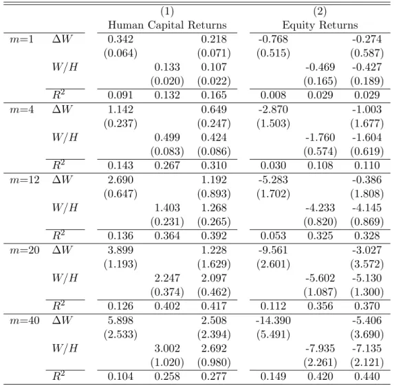
We use our human capital measures to forecast the returns to (1) human capital and (2) equity. Table 10 andTable 11 present the coefficients and R-squares of these estimates for real and excess returns, respectively, for quarterly data. Quarterly estimates are presented form={1,4,20,40}.49 The first row of eachmestimation only includes labor compensation growth (∆W); the second row only includes the labor compensation to human capital wealth ratio (W/H), while row three includes both regressors. Including onlyW/Hdominates only including ∆W at all horizons for human capital (column 1) and equity (column 2), for both real and excess returns. The fit of the model improves at longer horizons in general for
48For example, the end of Q1 human capital estimates to Q2 wage ratio is used to forecast the Q3 total
return, as the end of Q1 price is estimated using Q2 consumption to avoid any information overlapping.
returns, with the exception of moving from m = 20 to m = 40 for human capital returns (both real and excess).
The improved forecasting ability of the model for human capital returns at longer hori-zons matches whatCampbell and Shiller(1988) find in the case of stock returns. Moreover, this result holds when only including our “dividend to price ratio” (i.e., labor compensation to human capital wealth), while adding information, such as changes in “dividends” (labor compensation) does not improve the predictive power substantially.
The results for equity return predictability are impressive, especially in the long run. For example the R-square is 0.03 for 1 quarter excess returns, but increases to 0.33 for 12 quarter cumulative returns, and to 0.44 for 40 quarter cumulative returns. In addition, our point estimates for excess returns match those of Lettau and Ludvigson (2001) very closely. In our setup, our estimated coefficient on the labor compensation to wealth ratio should be equal to the estimated coefficient on caydt times −βy = −0.59 in Lettau and Ludvigson (2001) as implied by equation (13). For example, our 12 quarter cumulative return estimated coefficient is −4.23, while Lettau and Ludvigson’s coefficient on caydt is
8.57, implying an estimate of around−5.05 in our framework.
Given this evidence, and that our measure of human capital wealth is arguably best approximated in the long run, we find these regression results to be further evidence that our measure of human capital wealth is a good one.
5
Conclusion
We propose a simple methodology to recover the value of human capital based on the assumption of a constant consumption to total wealth ratio. Total wealth consists of non-human capital and non-human capital. Given an assumed value of a consumption to wealth ratio, it is straightforward to recover the value of human capital wealth when non-human capital data is available.
We apply the methodology to the U.S. and nine other OECD countries. While our assumption may be viewed as overly restrictive, our estimates of the value of human capital wealth look quite reasonable in many respects. We find that human capital wealth represents approximately 75 percent of total wealth, which is almost the same as the labor share to national income ratio. Because labor income is more stable than capital income, our finding seems reasonable. Moreover, the value of human capital and labor compensation are cointegrated, which also provides support the assumption underlying thecay approach proposed by Lettau and Ludvigson (2001). Average growth rates of human capital are
in line with those found in existing literature, while level estimates differ. However, our estimates and Jorgenson and Fraumeni (1989)’s are not so different once we remove non-market activity from their estimates. These findings provide support that our estimates are quite reasonable, and the notion that human capital is a discounted sum of future labor income.
We then characterize the basic properties of the total returns to human capital wealth using U.S. data. We find that human capital wealth is best characterized as low risk and high return. Furthermore, human capital is positively correlated with housing and long-term bonds, but negatively correlated with equity returns. The positive correlation with housing can provide a potential explanation for the relatively strong wealth effect of housing found in empirical work (given the theoretical ambiguity of the relationship), as housing prices may proxy for the value of human capital wealth. In addition, human capital’s positive correlation with long-term bonds can help justify observed households’ borrowing behavior, and the negative correlation with equity can help to explain the home bias in equity portfolio. While our characterization of human capital returns is based on simple statistics, it already provides some interesting facts. Furthermore, we are able to use our human capital wealth measures to predict both human capital and equity returns.
Future work will consider these relationships in more detail in light of our results, and examining the value of human capital wealth at the individual level also seems to be a fruitful line of research to pursue. Furthermore, our estimates of human capital can also be used to examine what type of shocks are driving innovations in human capital returns.
Appendix A
Detailed Derivations of Log-Linearized System
of Equations
A.1 Budget Constraint
The budget constraint can be written as
Wt+1=Rm,t+1(Wt−Ct), (A.1)
where Rm,t+1 is the gross return on total assets from time tto time t+ 1, and Wt is total
assets including human capital wealth and non-human capital wealth. Non-human capital wealth includes both financial assets and non-financial assets such as housing.
First, rewrite(A.1) as
Wt+1 Wt =Rm,t+1 1− Ct Wt
and take logarithms of both sides to get ∆wt+1=rm,t+1+ ln 1−exp ln Ct Wt . (A.2)
Taking the first-order Taylor approximation of (A.2)we obtain: ∆wt+1 =rm,t+1+ ln 1−exp ln C W − exp ln C W 1−exp ln WC ct−wt−ln C W , (A.3) where ln(WC) is the logarithm of the steady-state consumption to wealth ratio. Define
ρ≡1−exp ln C W = W −C W k≡ln(ρ)− 1− 1 ρ ln(1−ρ)
and substituteρ and k into(A.3)to arrive at ∆wt+1 =rm,t+1+ 1−1 ρ (ct−wt) +k. (A.4)
Using the fact that ∆wt+1= (ct−wt)−(ct+1−wt+1) + ∆ct+1, we can rearrange (A.4)as:
ct−wt=ρ[(ct+1−wt+1) +rm,t+1−∆ct+1+k]. (A.5)
Taking timetconditional expectations of both sides of (A.5)and solving forward, we arrive at(3): ct−wt=Et ∞ X j=1 ρj(rm,t+j−∆ct+j) + ρk 1−ρ, (A.6)