An R Library to construct empirical likelihood
confidence intervals for complex estimators
Yves G. Berger, University of Southampton, UK
Keywords: Calibration, Design-based approach, Estimating equations, Finite population corrections, Hajek estimator, Horvitz-Thompson estimator, Regression estimator, Stratification, Unequal inclusion probabilities.
We developed an R library which can be used to compute empirical likelihood point estimates and confidence intervals. After explaining the empirical likelihood theory, we show how to use this library and an example based on the 2009 EU-SILC survey.
1. INTRODUCTION
Under complex sampling designs, point estimators may not have a normal sampling distributionand linearised variance estimators may be biased. Hence standard confidence intervals based upon the central limit theorem may have poor coverages. We propose an empirical likelihood approach which gives design based confidence intervals. The proposed approach does not rely on the normality of the point estimator, variance estimates, design-effects, re-sampling, joint- inclusion probabilities and linearisation, even when the estimator of interest is not linear. It can be used to construct confidence intervals for a large class of complex sampling designs and complex estimators which are solution of an estimating equation [4]. It can be used for means, regressions coefficients, quantiles, totals or counts even when the population size is unknown. It can be used with large and negligible sampling fractions. It also provides asymptotically optimal point estimators, and naturally includes calibration constraints [2]. The proposed approach is computationally simpler than the pseudo empirical likelihood [9] and the bootstrap approaches [8]. Berger and De La Riva Torres [1] show that the empirical likelihood confidence interval may give better coverages than the approaches based on linearisation [3], bootstrap [8] and pseudo empirical likelihood [9].
2. EMPIRICAL LIKELIHOOD APPROACH
Let be a finite population of units; where is a fixed quantity which is not necessarily known. Suppose that the population parameter of interest is the unique solution of the following estimating equation [4].
where is a function of and of the characteristics of the unit , such as the variables of interests and the auxiliary variables.
where denotes the sum over the sampled units. The quantities are unknown positive scale loads. The maximum likelihood estimators of are the values which maximise subject to the constraints and
where is vector associated with the -th sampled unit and is vector (see Section 2.1). The values are survey weights.
2.1. Maximum empirical likelihood estimator
Suppose that the finite population is stratified into strata denoted by ; where . Suppose that a sample of fixed size is selected with replacement with unequal probabilities from . Let and ; where are the values of the design (or stratification) variables defined by , where denotes the vector of the strata sample sizes, with when and otherwise. It can be shown that . Let be the maximum value of the empirical log-likelihood function.
Let be the values which maximise subject to the constraints and with and , for a given . Let . The empirical log-likelihood ratio function (or deviance) is defined by the following function of .
The maximum empirical likelihood estimate of is defined by the value of which
minimises the function . As the minimum value of is zero, is the solution of . It can be easily shown that this implies that is the solution of the following estimating equation.
when , we have and is the
Horvitz-Thompson estimator [6] given by . When , is the Hajek [5] ratio estimator , where .
2.2. Empirical likelihood confidence intervals
Berger and De La Riva Torres [1] show that the random variable follows asymptotically a chi-squared distribution with one degree of freedom. Thus, the level empirical likelihood confidence interval for the population parameter is given by
.
Note that is a convex non-symmetric function with a minimum when is the maximum empirical likelihood estimator. This interval can be found using a bisection search method. This involves calculating for several values of . Berger and De La Riva Torres [1] showed how this approach can be used to accommodate large sampling fractions and non-response.
It is also possible to calibrate towards parameters more complex than totals. For example, we may want to calibrate with respect to population means, quantiles or variances. In this case, the calibration constraint is specified by the estimating equations ; where is a vector function of the auxiliary variables and of a known parameter which is the solution of the following estimating equation
Calibration constraints are taken into account by including the auxiliary variables within the . In this case, we use and . For example, if we want to calibrate towards known population means , we need to use ; where is a vector of known population totals. Simultaneous calibration on totals, means, proportion or any known parameter is also feasible.
3. AN R LIBRARY
In order to implement the approach describes in Section 2, we developed a library in R called emplikfpop. First, we need to specify the design and calibration variables. Secondly, we need to specify the parameter of interest (i.e. the definition of ) and the finite population correction. This information is needed for point estimation and for confidence intervals.
i. Design and auxiliary information: This information is contained in the matrix
and the vector . is a matrix containing the stratification labels, the and (depending on ). The vector
gives the columns (in ) of stratification and .
ii. Definition of the parameter of interest: A function object defining the
function . This function depends on a matrix and a vector
which specify the data needed in the definition of . This function also depends on , a given value for . This function has the following format:
iii. Finite population corrections: The vector contains the or
or 1 (if the finite population correction is ignored).
iv. Survey weights: The survey weight are computed using the function
v. Point estimate: The point estimate is computed using the following function
where and specify the range of .
vi. Confidence interval: The confidence interval is computed using the following
function
where is the level of the confidence interval. For example, for the 95% confidence interval, we use . The object contains the bounds of the confidence interval. We have also predefined function for means,
totals and quantiles: , and
For the Rao-Hartley-Cochran sampling design, we have the
4. AN APPLICATION TO THE EU-SILC HOUSEHOLD SURVEY
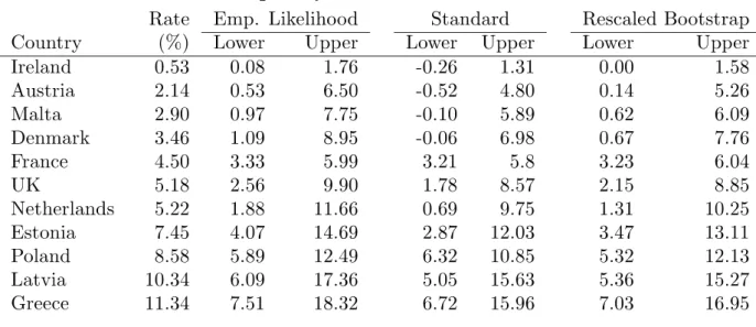
We use the 2009 EU-SILC user database to estimate the persistent at-risk-of-poverty rate. we adopted an ultimate cluster approach, where the units are the primary sampling units. In the table below, we have the point estimate and several confidence intervals for a couple of countries: the empirical likelihood confidence intervals, the standard confidence intervals based on variance estimates and the rescaled bootstrap confidences intervals [8]. Note that the bounds of the standard intervals are negative for Ireland, Austria, Malta and Denmark. The bootstrap bounds and the empirical likelihood bounds are larger than the bounds of the standard intervals. These differences are more pronounced for Austria, Malta, Denmark, the Netherlands, Estonia, Latvia and Greece. This is due to the skewness of the sampling distribution.
Table 1: Persistent at-risk-of-poverty rate & confidence intervals. 2009 EU-SILC.
REFERENCES
[1] Berger, Y. G. and De La Riva Torres, O. (2012) Empirical likelihood confidence intervals for complex sampling designs. S3RI Working paper,
http://eprints.soton.ac.uk/337688/
[2] Deville, J. C. and Sarndal (1992) Calibration estimators in survey sampling. Journal of the American Statistical Association, 87, 376-382.
[3] Deville, J. C. (1999) Variance estimation for complex statistics and estimators: linearization and residual techniques. Survey Methodology, 25} 193-203.
[4] Godambe, V. P. (1960) An optimum property of regular maximum likelihood estimation. The Annals of Mathematical Statistics, 31, 1208-1211.
[5] Hajek, J. (1971) Comment on a paper by D. Basu. in Foundations of Statistical Inference. Toronto: Holt, Rinehart and Winston.
[6] Horvitz, D. G. and Thompson, D. J. (1952) A generalization of sampling without replacement from a finite universe. Journal of the American Statistical Association, 47, 663-685.
[7] Owen, A. B. (2001) Empirical Likelihood. New York: Chapman & Hall.
[8] Rao, J. N. K., Wu, C. F. J. and Yue, K. (1992) Some recent work on resampling methods for complex surveys. Survey Methodology, 18, 209--217.
[9] Wu, C. and Rao, J. N. K. (2006) Pseudo-empirical likelihood ratio confidence intervals for complex surveys. The Canadian Journal of Statistics, 34, 359-375.