GETTING THE MOST OUT OF YOUR DATA:
MULTITASK BAYESIAN NETWORK STRUCTURE
LEARNING, PREDICTING GOOD PROBABILITIES
AND ENSEMBLE SELECTION
A Dissertation
Presented to the Faculty of the Graduate School of Cornell University
in Partial Fulfillment of the Requirements for the Degree of Doctor of Philosophy
by
Alexandru Niculescu-Mizil August 2008
c
2008 Alexandru Niculescu-Mizil ALL RIGHTS RESERVED
GETTING THE MOST OUT OF YOUR DATA: MULTITASK BAYESIAN NETWORK STRUCTURE LEARNING, PREDICTING GOOD
PROBABILITIES AND ENSEMBLE SELECTION Alexandru Niculescu-Mizil, Ph.D.
Cornell University 2008
First, I consider the problem of simultaneously learning the structures of mul-tiple Bayesian networks from mulmul-tiple related datasets. I present a multitask Bayes net structure learning algorithm that is able to learn more accurate network structures by transferring useful information between the datasets. The algorithm extends the score and search techniques used in traditional structure learning to the multitask case by defining a scoring function for sets of structures (one struc-ture for each task) and an efficient procedure for searching for a high scoring set of structures. I also address the task selection problem in the context of multitask Bayes net structure learning. Unlike in other multitask learning scenarios, in the Bayes net structure learning setting there is a clear definition of task relatedness: two tasks are related if they have similar structures. This allows one to automati-cally select a set of related tasks to be used by multitask structure learning.
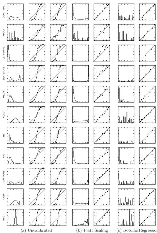
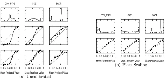
Second, I examine the relationship between the predictions made by differ-ent supervised learning algorithms and true posterior probabilities. I show that quasi-maximum margin methods such as boosted decision trees and SVMs push probability mass away from 0 and 1 yielding a characteristic sigmoid shaped distor-tion in the predicted probabilities. Naive Bayes pushes probabilities toward 0 and 1. Other models such as neural nets, logistic regression and bagged trees usually do not have these biases and predict well calibrated probabilities. I experiment
with two ways of correcting the biased probabilities predicted by some learning methods: Platt Scaling and Isotonic Regression. I qualitatively examine what dis-tortions these calibration methods are suitable for and quantitatively examine how much data they need to be effective.
Third, I present a method for constructing ensembles from libraries of thou-sands of models. Model libraries are generated using different learning algorithms and parameter settings. Forward stepwise selection is used to add to the ensem-ble the models that maximize its performance. The main drawback of ensemensem-ble selection is that it builds models that are very large and slow at test time. This drawback, however, can be overcome with little or no loss in performance by using model compression.
BIOGRAPHICAL SKETCH
Alexandru Niculescu-Mizil is a Ph.D. candidate in the Computer Science depart-ment at Cornell University. He received a Masters of Science degree in Computer Science from Cornell University and a Magna Cum Laude Bachelors degree in Mathematics and Computer Science from University of Bucharest. His research interests are in machine learning and data mining. He conducted research in induc-tive transfer, graphical model structure learning, probability estimation, empirical evaluations, ensemble methods, and on-line learning. He was awarded a Distin-guished Student Paper Award at the twenty second International Conference on Machine learning for the paper “Predicting Good Probabilities with Supervised Learning”, and a Best Student Paper Award at the Conference on Learning The-ory for the paper “Regret Bounds for Sleeping Experts and Bandits”.
ACKNOWLEDGMENTS
I am grateful to have had Rich Caruana as my advisor. He taught me all I know about research. I thank him for the countless hours he spent side by side with me showing me how to run experiments, how to interpret results, how to write a paper, and so on. I thank him for all the guidance and advice he gave me over the years, and for teaching me not only how to do good research, but also how to be a good researcher. Many thanks also go to the rest of my committee, especially to Thorsten Joachims. I thank Lillian Lee for her advice and support, and Robert Kleinberg for encouraging me to engage in theoretical machine learning research.
I thank my office mates –Andre Allavena, Eric Breck, Steve Chong, Jeff Hart-line, Filip Radlinski, and Matthew Schultz–, and the “guys next door” –Tom Finley, Art Munson, Daria Sorokina, and Benyah Shaparenko– for the countless academic and non-academic discussions, for putting up with me, and, above all, for being true friends. I thank Cindy Robinson for the fun chats we had over the years. Going to her office always brightened my day.
A great deal of gratitude goes to my family and friends in Romania. I thank my parents for the education they gave me over the years and for guiding me toward an academic career. I thank my best friend, Andrei Vlagali, who helped me keep my sanity on several occasions. My love goes to Alina, who came to live with me in Ithaca, even though this meant leaving behind her family and friends. Without her love and care I would have never made it. Last, but most important, I thank Ema, for the joy and excitement she brought to my life.
TABLE OF CONTENTS
Bibliographical Sketch . . . iii
Acknowledgments . . . v
List of Tables . . . viii
List of Figures . . . x
1 Overview 1 2 Inductive Transfer for Bayesian Network Structure Learning 5 2.1 Introduction . . . 5
2.2 Learning Bayes Nets from Data . . . 7
2.3 Learning from Multiple Related Tasks . . . 9
2.3.1 The Prior . . . 10
2.3.2 Greedy Structure Learning . . . 13
2.3.3 Searching for the Best Configuration . . . 14
2.3.4 Empirical Evaluation . . . 17
2.4 Task Selection for Multitask Structure Learning . . . 29
2.4.1 A Direct Measure of Task Relatedness . . . 31
2.4.2 An Indirect Measure of Task Relatedness . . . 32
2.4.3 Empirical Evaluation . . . 33
2.5 Discussion and Related Work . . . 42
2.6 Conclusions . . . 44
3 Predicting Good Probabilities with Supervised Learning 49 3.1 Introduction . . . 49
3.2 Calibration Methods . . . 50
3.2.1 Platt Calibration . . . 50
3.3 Qualitative Analysis of Predictions . . . 53
3.3.1 Boosting . . . 55
3.3.2 Support Vector Machines . . . 64
3.3.3 Artificial Neural Networks and Logistic Regression . . . 66
3.3.4 Decision Trees . . . 68
3.3.5 Bagged Decision Trees and Random Forests . . . 71
3.3.6 Memory Based Learning . . . 73
3.3.7 Naive Bayes . . . 75
3.4 Quantitative Analysis of Performance . . . 77
3.5 Learning Curve Analysis . . . 80
3.6 Conclusions . . . 83
3.A Histograms of Predicted Values and Reliability Diagrams . . . 86
4 Ensemble Selection 98 4.1 Introduction . . . 98
4.2 Improving Ensemble Selection . . . 100
4.2.1 Selection with Replacement . . . 100
4.2.2 Sorted Ensemble Initialization . . . 101
4.2.3 Bagged Ensemble Selection . . . 102
4.3 Experimental Evaluation . . . 102
4.3.1 Methodology . . . 102
4.3.2 Empirical Results . . . 105
4.3.3 Analysis of Training Size . . . 106
4.3.4 Cross-Validated Ensemble Selection . . . 109
4.3.5 Direct Metric Optimization . . . 113
4.3.6 Model Library Pruning . . . 115
4.5 Conclusions . . . 123
4.A Data Sets . . . 129
4.B Learning Algorithms . . . 129
4.C Performance Metrics Used . . . 131
LIST OF TABLES
3.1 PAV Algorithm . . . 53
4.1 Performance with and without model calibration. The best score in each column is bolded. . . 105
4.2 Performance with and without cross-validation for ensemble selec-tion and model selecselec-tion. . . 110
4.3 Percent loss reduction by dataset. . . 110
4.4 Breakdown of improvement from cross-validation. . . 112
4.5 Performance of ensemble selection when forced to optimize to one set metric. . . 115
4.6 Time in seconds to classify 10k cases. . . 120
4.7 Size of the models in MB. . . 121
4.8 RMSE results. . . 121
4.9 Description of problems . . . 130
4.10 Scales used to compute normalized scores. Each entry shows bot-tom / top for the scale. . . 135
LIST OF FIGURES
2.1 North American Bird Conservation Regions. . . 19 2.2 Reduction in edit distance (left) and KL-Divergence (right) for
ALARM . . . 22 2.3 Reduction in edit distance (left) and KL-Divergence (right) for
INSURANCE-IND . . . 23 2.4 Edit distance (left) and KL-Div (right) for different multitask priors 24 2.5 Edit distance (left) and KL-Div (right) for STL, learning identical
structures and MTL . . . 24 2.6 The true structures (left), structures learned by MTL (middle) and
STL (right) for ALARM-COMP . . . 26 2.7 Edit distance (left) and KL-Divergence (right) vs. train set size for
ALARM-COMP. . . 27 2.8 Average mean log likelihood vs. the penalty parameter for
multi-task structure learning on the BIRD problem. . . 28 2.9 Average mean log likelihood vs. training set size for the BIRD
problem. . . 29 2.10 KL-Divergence of the principal task vs. the number of selected
tasks for the ALARM-COMP problem. . . 34 2.11 Improvement in Edit Distance over single task learning vs. training
set size for the ALARM-COMP problem. . . 36 2.12 Distance between the principal task and the rest of the tasks for
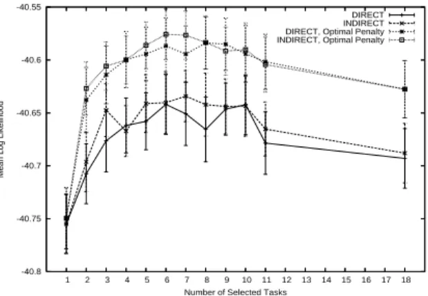
one trial of the ALARM-COMP problem. Distance is computed using the direct measure. . . 37 2.13 Mean log likelihood vs. the number of selected tasks for BCR28 on
the BIRD problem. . . 38 2.14 Average improvement in mean log likelihood over single task
learn-ing vs. trainlearn-ing set size for task selection on the BIRD problem (average over 11 BCRs). . . 39 2.15 Average improvement in mean log likelihood over single task
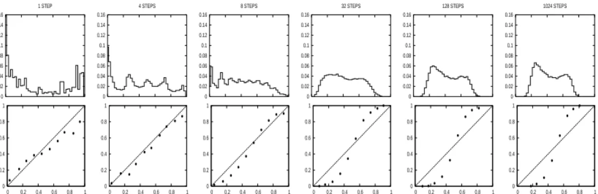
learn-ing vs. trainlearn-ing set size for task clusterlearn-ing on the BIRD problem (average over 11 BCRs). . . 40 2.16 Cluster hierarchy for the BIRD problem. . . 41 3.1 Effect of boosting on the predicted values. Histograms of the
pre-dicted values (top) and reliability diagrams (bottom) on the test set for boosted trees at different steps of boosting on the COV TYPE problem. . . 56 3.2 Histograms of predicted values and reliability diagrams for boosted
decision trees before and after calibration. . . 57 3.3 Histograms of predicted values and reliability diagrams for boosted
3.4 Histograms of predicted values and reliability diagrams for (a)boosted trees and (b)boosted stumps calibrated with Logistic Correction. . 61 3.5 Histograms of predicted values and reliability diagrams for (a)boosted
trees and (b)boosted stumps trained to directly optimize log-loss. . 61 3.6 Histograms of predicted values and reliability diagrams for SVMs
before and after calibration. . . 64 3.7 Histograms of predicted values and reliability diagrams for neural
networks before and after calibration. . . 66 3.8 Histograms of predicted values and reliability diagrams for (a)Decision
Trees, (b)Bagged Decision Trees and (c)Random Forests . . . 69 3.9 Histograms of predicted values and reliability diagrams after
cali-bration with Platt Scaling for (a)Bagged Decision Trees and (b)Random Forests. . . 73 3.10 Histograms of predicted values and reliability diagrams for memory
based learning before and after calibration. . . 74 3.11 Histograms of predicted values and reliability diagrams for Naive
Bayes before and after calibration. . . 76 3.12 Performance of learning algorithms . . . 78 3.13 Learning Curves for Platt Scaling and Isotonic Regression (averages
across 10 problems). . . 81 3.14 Histograms of predicted values and reliability diagrams for boosted
decision stumps before and after calibration. . . 87 3.15 Histograms of predicted values and reliability diagrams for boosted
decision stumps calibrated with Logistic Regression and for boosted decision stumps trained to optimize log-loss. . . 88 3.16 Histograms of predicted values and reliability diagrams for boosted
decision trees calibrated with Logistic Regression and for boosted decision trees trained to optimize log-loss. . . 89 3.17 Histograms of predicted values and reliability diagrams for SVMs
before and after calibration. . . 90 3.18 Histograms of predicted values and reliability diagrams for artificial
neural networks before and after calibration. . . 91 3.19 Histograms of predicted values and reliability diagrams for logistic
regression before and after calibration. . . 92 3.20 Histograms of predicted values and reliability diagrams for decision
trees before and after calibration. . . 93 3.21 Histograms of predicted values and reliability diagrams for bagged
decision trees before and after calibration. . . 94 3.22 Histograms of predicted values and reliability diagrams for random
forests before and after calibration. . . 95 3.23 Histograms of predicted values and reliability diagrams for memory
based learning before and after calibration. . . 96 3.24 Histograms of predicted values and reliability diagrams for naive
4.1 Selection With and Without Replacement. . . 101 4.2 Learning curves for ensemble selection with and without bagging,
and for picking the best single model (modsel). . . 108 4.3 Scatter plots of ensemble selection performance when RMS is
op-timized (x-axis) vs when the target metric is optimized (y-axis). Points above the line indicate better performance by optimizing to the target metric (e.g. accuracy) then when optimizing RMS. Each point represents a different data set; circles are averages for a prob-lem over 5 folds, and X’s are performances using cross-validation. Each metric (and the mean across metrics) is plotted separately. . 114 4.4 Pruned ensemble selection performance. . . 117 4.5 RMS performance for pruned ensemble selection. . . 118
CHAPTER 1
OVERVIEW
The first part of this dissertation is concerned with Bayesian network structure learning. Bayesian networks are a standard tool for reasoning with uncertainty that encode compactly the probabilistic relationships between variables of inter-est. Bayes nets are specified by a directed acyclic graph (DAG), called the Bayes net structure, that encodes the statistical dependence and independence relation-ships between the variables, and a set of parametrized conditional probability functions. Learning the dependency structure from data provides invaluable infor-mation about the domain, making Bayesian networks a very powerful data analysis tool. For instance, learning a Bayes net from bird sighting data can help ecologists and ornithologists understand how environmental and human factors influence the abundance of different bird species. Or, learning a Bayes net from gene expression data can give microbiologists insights into the gene regulatory system.
My work is motivated by the observation that in many situations data is avail-able for multiple related problems. Bird sighting data is availavail-able for different, ecologically distinct, regions in North America; gene expression data is available for multiple species. If the dependency structures of the related problems are similar, then useful information can be transfered among problems. Specifically, finding a direct statistical dependency (or lack thereof) between two variables in one problem provides additional evidence for the same relationship in the other problems. Chapter 2 presents a Bayesian network structure learning technique that is able to leverage this additional evidence in a principled manner. When compared to the traditional approach of learning the structures for each domain in isolation, without inter-problem transfer, my technique recovers significantly more accurate dependency structures, especially in situations where the data is scarce.
Part of this work has been presented in (Niculescu-Mizil & Caruana, 2007). Another problem I address in this dissertation is that of predicting accurate class membership probabilities with supervised classification methods. The over-whelming majority of the work in supervised classification has focused on predict-ing the “correct” class for a given instance. In many cases, however, there is no “correct” class, but rather the instance has a certain probability of membership in each of the classes. Being able to accurately estimate these membership prob-abilities is required by many applications. This ability is key, for instance, when the predictions are used in a decision making process, when classifiers are used as parts of larger systems, or when dealing with varying misclassification costs.
In Chapter 3 I analyze the ability of predicting accurate class membership probabilities of several widely used supervised learning algorithms. The analy-sis shows that a number of learning algorithms, including boosted decision trees, support vector machines, and Naive Bayes, predict inaccurate class membership probabilities. This makes them unusable in applications where probability esti-mation is critical. To address this problem, I investigate techniques that “fix” the predictions of these learning algorithms transforming them into accurate class membership probability estimates. Parts of this chapter have been presented in (Niculescu-Mizil & Caruana, 2005b), and (Niculescu-Mizil & Caruana, 2005a).
The last chapter tackles the issue of obtaining high performing classifiers. Even small improvements in the performance of a classifier can lead to large gains if the classifier is widely used. Consider, for instance, credit card fraud detection, where a classifier would be used to distinguish fraudulent transactions from authentic ones. Since credit card companies process billions of transactions every year, even small improvements in the performance of the used classifier result in large gains from preventing fraudulent transactions and avoiding frustrating honest customers.
Ensembles of classifiers, meta-classifiers that combine the predictions of a set
of base classifiers in order to obtain higher performance, have proved to be very
effective at obtaining high performing classifiers. In Chapter 4 I presentEnsemble
Selection, an ensemble learning technique that yields some of the most powerful,
high performing, general purpose classifiers to date. The work in this chapter has been presented in (Caruana et al., 2004), (Caruana et al., 2006) and (Bucila et al., 2006).
BIBLIOGRAPHY
Caruana, R., Munson, A., & Niculescu-Mizil, A. (2006). Getting the most out of
ensemble selection(Technical Report 2006-2045). Cornell University. Full version
of paper published at ICDM 2006.
Caruana, R., Niculescu-Mizil, A., Crew, G., & Ksikes, A. (2004). Ensemble selec-tion from libraries of models. Proc. 21st International Conference on Machine
Learning (ICML’04).
Fawcett, T., & Niculescu-Mizil, A. (2007). PAV and the ROC convex hull.Machine
Learning,68, 97–106.
Niculescu-Mizil, A., & Caruana, R. (2005a). Obtaining calibrated probabilities from boosting. Proc. 21st Conference on Uncertainty in Artificial Intelligence
(UAI ’05). AUAI Press.
Niculescu-Mizil, A., & Caruana, R. (2005b). Predicting good probabilities with supervised learning. Proc. 22nd International Conference on Machine Learning
(ICML’05)(pp. 625–632).
Niculescu-Mizil, A., & Caruana, R. (2007). Inductive transfer for bayesian network structure learning. Proc. 11th International Conf. on AI and Statistics.
CHAPTER 2
INDUCTIVE TRANSFER FOR BAYESIAN NETWORK STRUCTURE LEARNING
2.1
Introduction
Bayes Nets (Pearl, 1988) provide a compact, intuitive description of the depen-dency structure of a domain by using a directed acyclic graph to encode proba-bilistic dependencies between variables. This intuitive encoding of the dependency structure makes Bayes Nets appealing in expert systems where expert knowledge can be encoded through hand-built dependency graphs. Acquiring expertise from humans, however, is difficult and expensive, so significant research has focused on learning Bayes Nets from data. The learned dependency graph also provides useful information about a problem and is often used as a data analysis tool. For exam-ple Friedman et al. (2000) used Bayes Nets learned from gene expression data to discover regulatory interactions between genes for a species of yeast.
Until now, Bayes Net structure learning research has focused on learning the dependency graph for one problem in isolation. In many situations, however, data is available for multiple related problems. In these cases, inductive transfer (Caru-ana, 1997; Baxter, 1997; Thrun, 1996) suggests that it may be possible to learn more accurate dependency graphs by transferring information between problems. For example, suppose that we want to learn the gene regulatory structure for a number of yeast species. Since the regulatory structures are very similar, learn-ing that there is an interaction between two genes in one species of yeast should provide evidence for the existence of the same interaction in the other species.
In this chapter, we present an algorithm for learning the Bayes Net structures for multiple related tasks simultaneously. The method assumes that the true
struc-tures of the related tasks are similar. When this assumption is true, the presence or absence of arcs in some of the structures provides evidence for the presence or absence of those same arcs in the other structures. By taking into account such ev-idence the multitask structure learning algorithm we propose is able to learn more accurate network structures than its single-task structure learning counterpart.
We also tackle the task selection problem for multitask structure learning. Task selection is an important, but hard, problem in inductive transfer: given a set of tasks, select a subset to use as related tasks in a multitask learner. The main rea-son why automatic task selection is difficult in a general multitask learning setting is that there is no clear definition of task relatedness. Even if there exists an intu-itive notion of task relatedness, it might be difficult to quantify. Furthermore the intuitive notion of relatedness might not correspond to a type of relatedness that the multitask learning algorithm is able to take advantage of. For example, playing tennis and running are, intuitively, related tasks, but if the particular multitask learning algorithm used can only transfer information about arm movements then multitask learning might not provide a benefit.
Unlike in the general case, in the multitask structure learning setting there exists a clear, quantifiable notion of task relatedness: two tasks are related if their structures are similar. Moreover, this is exactly the type of relatedness the mul-titask structure learning algorithm we study in this chapter takes advantage of. While computing task relatedness this way is not feasible since the true struc-tures are unknown, it is possible to compute a good approximation using only the available data. We propose two such measures of task relatedness and a task selection algorithm for multitask structure learning. We show that, by selecting an appropriate set of tasks to use as related tasks, task selection further improves the performance of multitask structure learning.
The chapter starts with an overview of Bayes Net structure learning for a single problem, then describes the new multitask structure learning algorithm in Section 2.3. Section 2.3.4 provides an empirical evaluation of the new algorithm. Section 2.4 presents two task relatedness measures and the task selection algo-rithm. Empirical results supporting our task selection method are presented in Section 2.4.3. The chapter ends with an overview of related work in Section 2.5 and final conclusions in Section 2.6.
2.2
Learning Bayes Nets from Data
A Bayesian NetworkB ={G, θ} that encodes the joint probability distribution of a set ofn random variables X ={X1, X2, ..., Xn}is specified by a directed acyclic
graph (DAG) G and a set of conditional probability functions parametrized by θ
(Pearl, 1988). The Bayes Net structure, G, encodes the probabilistic dependencies in the data: the presence of an edge between two variables means that there exists a direct dependency between them. An appealing feature of Bayes Nets is that the dependency graphGis easy to interpret and can be used to aid understanding the problem domain.
Given a dataset D = {x1
, ..., xm} where each xi is a complete assignment of
variablesX1, ..., Xn, it is possible to learn both the structure Gand the parameters
θ(Cooper & Hersovits, 1992; Heckerman, 1999). Following the Bayesian paradigm, the posterior probability of the structure given the data is estimated via Bayes rule:
P(G|D)∝P(G)P(D|G) (2.1)
The prior P(G) indicates the belief before seeing any data that the structure
Gis correct. If there is no reason to prefer one structure over another, one should assign the same probability to all structures. This uninformative (uniform) prior is
rarely accurate, but often is used for convenience. If there exists a known ordering on the nodes in G such that all the parents of a node precede it in the ordering, a prior can be assessed by specifying the probability that each of the n(n−1)/2 possible arcs is present in the correct structure (Buntine, 1991). Alternately, when there is access to a structure believed to be close to the correct one (e.g. from an expert), P(G) can be specified by penalizing each difference between G and the given structure by a constant factor (Heckerman et al., 1995).
The marginal likelihood, P(D|G), is computed by integrating over all possible parameter values:
P(D|G) =
Z
P(D|G, θ)P(θ|G)dθ (2.2)
When the local conditional probability distributions are from the exponential family, the parameters θi are mutually independent, we have conjugate priors for
these parameters, and the data is complete, P(D|G) can be computed in closed form (Heckerman, 1999).
Treating P(G|D) as a score, one can search for a high scoring network using heuristic search (Heckerman, 1999). Greedy search, for example, starts from an initial structure, evaluates the score of all theneighborsof that structure and moves to the neighbor with the highest score. The search terminates when the current structure is better than all it’s neighbors. Because it is possible to get stuck in a local minima, this procedure usually is repeated a number of times starting from different initial structures. A common definition of the neighbors of a structure G is the set of all the DAGs that can be obtained by removing or reversing an existing arc in G, or by adding an arc that is not present in G.
2.3
Learning from Multiple Related Tasks
In the previous section we reviewed how to learn a Bayes Net for a single task. What if instead of a single task we have a number of related tasks (e.g., gene expression data for a number of related species) and we want to learn a Bayes Net structure for each of them?
Given k data-sets, D1, ..., Dk, defined on overlapping but not necessarily
iden-tical sets of variables, we want to learn the structures of the Bayes Nets B1 =
{G1, θ1}, ...,Bk ={Gk, θk}, one for each data-set. In what follows, we will use the
term configurationto refer to a set of structures (G1, ..., Gk).
From Bayes rule, the posterior probability of a configuration given the data is:
P(G1, ..., Gk|D1, ..., Dk)∝P(G1, ..., Gk)P(D1, ..., Dk|G1, ..., Gk) (2.3)
The marginal likelihood P(D1, ..., Dk|G1, ..., Gk) is computed by integrating
over all parameter values for all thek networks:
P(D1, ..., Dk|G1, ..., Gk) = = Z P(D1, ..., Dk|G1, ..., Gk, θ1, ..., θk)× (2.4) P(θ1, ..., θk|G1, ..., Gk)dθ1...dθk = Z P(θ1, ..., θk|G1, ..., Gk) k Y p=1 P(Dp|Gp, θp)dθ1...dθk
If we make the parameters of different networks independent a priori (i.e.
P(θ1, ..., θk|G1, ..., Gk) = P(θ1|G1)...P(θk|Gk) ), the marginal likelihood becomes
just the product of the marginal likelihoods of each data set given its network structure. In this case the posterior can be written as:
P(G1, .., Gk|D1, .., Dk)∝P(G1, .., Gk) k
Y
p=1
Making the parameters independent a priori is unfortunate, and contradicts the intuition that related tasks should have related parameters, but it is needed in order to make structure learning efficient (see Section 2.3.3). It is important to note that this is not a restriction on the model. Unlike the Naive Bayes model for example, where the attribute independence assumption actually restricts the class of models that can be learned, here the learned parameters will be correlated if such correlation is present in the data. The only downside of making the parameters independent a priori is that it prevents multitask structure learning from taking advantage of the similarities between the parameters of different tasks during the structure learning phase. After the structures have been learned, however, such similarities could be leveraged to learn more accurate parameters. Finding ways to allow for somea priori parameter dependence while still maintaining computa-tional efficiency is an interesting direction for future work.
2.3.1
The Prior
The prior knowledge of how related the different tasks are and how similar their structures should be is encoded in the priorP(G1, ..., Gk). If there is no reason to
believe that the structures for each task should be related, thenG1, ..., Gk should
be made independent a priori (i.e. P(G1, ..., Gk) = P(G1)·...·P(Gk)). In this
case the structure-learning can be done independently for each task using the corresponding data set.
At the other extreme, if the structures for all the different tasks should be iden-tical, the priorP(G1, ..., Gk) should put zero probability on any configuration that
contains nonidentical structures. In this case one can efficiently learn the same structure for all tasks by creating a new data set with attributes X1, ..., Xn, T SK,
where T SK encodes the task the case is coming from.1 Then learn the structure
1
for this new data set under the restriction thatT SK is always the parent of all the other nodes. The common structure for all the tasks is exactly the learned struc-ture, with the nodeT SK and all the arcs connected to it removed. This approach, however, does not easily generalize to the case where tasks have only partial over-lap in their attributes. The algorithm proposed below avoids this problem, while computing the same solution when structures are forced to be identical.
Between these two extremes, the prior should encourage finding similar network structures for the tasks. The prior can be seen as penalizing structures that deviate from each other, so that deviation will occur only if it is supported by enough evidence in the data.
One way to generate such a prior for two structures is to penalize each arc (Xi, Xj) that is present in one structure but not in the other by a constantδ∈[0,1]:
P(G1, G2) = Zδ·(P(G1)P(G2)) 1 1+δ Y (Xi,Xj)∈ G1∆G2 (1−δ) (2.6)
whereZδis a normalization factor that is absorbed in the proportionality constant
of equation 2.5, andG1∆G2 represents the symmetric difference between the edge sets of the two DAGs (arc reversals can be counted only once or twice).
Ifδ = 0 thenP(G1, G2) =P(G1)P(G2), so the structures are learned indepen-dently. If δ = 1 then P(G1, G2) = qP(G)P(G) = P(G) for G1 = G2 = G and
P(G1, G2) = 0 for G1 6=G2, leading to learning identical structures for all tasks.
Forδ between 0 and 1, the higher the penalty, the higher the probability of more similar structures. The advantage of this prior is that P(G1) and P(G2) can be any structure priors that are appropriate for the task at hand. If a variable,Xi, is
present in one structure but not in the other, then any arc that has Xi as one of
its extremities should not incur any penalty.
One way to interpret the above prior is that it penalizes byδeachedit (i.e. arc addition, arc removal or arc reversal) that is necessary to make the two structures identical (arc reversals can count as one or two edits). This leads to a natural extension to more than two tasks that penalizes each edit that is necessary to obtain a set of identical structures:
P(G1, ..., Gk) = Zδ,k· Y 1≤s≤k P(Gs) 1 1+(k−1)δ ×Y i,j (1−δ)editsi,j (2.7)
whereeditsi,j is the minimum number of edits necessary to make the edge between
Xi and Xj the same in all the structures. We will call this prior the Edit prior.
The exponent 1/(1 + (k −1)δ) is used to transition smoothly between the case where structures should be independent (i.e. P(G1, ..., Gk) = (P(G1)...P(Gk))1
for δ = 0) and the case where structures should be identical (i.e. P(G, .., G) = (P(G)...P(G))1/k forδ= 1). This prior can be easily generalized by using different
penalties for different edges (e.g. if certain edges should not chance between tasks then the penalty on those edged should be 1), and/or different penalties for different edit operations.
Another way to specify a prior for more than two tasks is to multiply the penalties incurred between all pairs of structures:
P(G1, ..., Gk) =Zδ,k · Y 1≤s≤k P(Gs) 1 1+(k−1)δ × Y 1≤s<t≤k Y (Xi,Xj)∈ Gs∆Gt (1−δ) 1 k−1 (2.8)
We will call this prior thePairedprior. The exponent 1/(k−1) is used because each individual structure is involved ink−1 terms (one for each other structure). One advantage that the Paired prior has over the Edit prior is that it can be generalized by specifying different penalties between different pairs of structures. This can handle situations where there is reason to believe that Task1 is related to
Task2, and Task2 is related to Task3, but the relationship to between Task1 and Task3 is weaker.
There are of course other priors that encourage finding similar networks for each task in different ways. In particular, if the process that generated the related tasks is know, it might be possible to design a suitable prior.
2.3.2
Greedy Structure Learning
Treating P(G1, ..., Gk|D1, ..., Dk) as a score, we can search for a high scoring
con-figuration using an heuristic search algorithm. If we choose to use greedy search for example, we start from an initial configuration, compute the scores of the neigh-boring configurations, then move to the configuration that has the highest score. The search ends when no neighboring configuration has a higher score than the current one.
One question remains: what do we mean by the neighborhood of a config-uration? An intuitive definition of a neighbor is the configuration obtained by modifying a single arc in a single DAG in the configuration, such that the re-sulting graph is still a DAG. With this definition, the size of the neighborhood of a configuration is O(k ∗n2
) for k tasks and n variables. Unfortunately, this definition creates a lot of local minima in the search space. Consider for example the case where there is a strong belief that the structures should be similar (i.e. the penalty parameter of the prior, δ, is near one resulting in a prior probability near zero when the structures in the configuration differ). In this case it would be difficult to take any steps in the greedy search since modifying a single edge for a single DAG would make it different from the other DAGs, resulting in a very low posterior probability (score).
the set of all configurations obtained by selecting two nodes, and for each structure in the configuration, add, remove, reverse, or leave unchanged the arc between the two selected nodes, under the restriction that the resulting structure remains a DAG. It is easy to see that there is a path between any two configurations, so the search space is connected. Given this definition, the size of a neighborhood is O(n2
3k), which is exponential in the number of tasks, but only quadratic in
the number of nodes.2 In the case where all the learned structures are required
to be identical (infinite penalty for diverging structures) multitask learning, with this definition of neighborhood, will find the same structures as the specialized algorithm described in Section 2.3.1. We will use this definition for the rest of the chapter.
2.3.3
Searching for the Best Configuration
At each iteration, the greedy procedure described in the previous section must find the best scoring configuration from a set N of neighboring configurations. In the naive approach the score of every configuration in N is computed and the configuration with the highest score is selected. Since the size ofN can get large for largenork, this naive approach can be very expensive. Much of this computation however can be avoided by using better search techniques to find the best scoring configuration.
Let a partial configuration of orderl,Cl= (G1, .., Gl), be a configuration where
only the structures for thefirstl tasks are specified and the rest ofk−l structures are not specified. We say that a configurationC matches a partial configurationCl
if the structures for the first l tasks in C are the same as the structures in Cl.
2
The restriction that changes, if any, have to occur between the same nodes in all the structures
could be dropped, but this would lead to a neighborhood that is exponential in both n and
k. Considering the assumption that the structures should be similar, such a restriction is not
A search strategy for finding the best scoring configuration in N can be repre-sented via a search tree of depth k that satisfies the following properties: a) each node at levellcontains a different valid partial configuration of orderl; b) all nodes in the subtree rooted at node Cl contain only (partial) configurations of order at
least l+ 1 that match Cl. (i.e. the first l structures are the same as inCl.)
If, given a partial configuration, the score of any complete configuration that matches it can be efficiently upper bounded, and the upper bound is lower than the current best score, then the entire subtree rooted at the respective partial con-figuration that can be pruned. This suggests using a branch and bound procedure for finding the best scoring configuration in N, by using deep first search and pruning the current subtree whenever possible. This branch and bound search sig-nificantly reduces the number of partial configurations (and consequently complete configurations) that need to be explored.
Let editsl,i,j be the minimum number of edits necessary to make the edge
between Xi and Xj the same in the first l structures, and let
Bestq = max{P(Gq)
1
1+(k−1)δP(D
q|Gq)}.
If the marginal likelihood of a configuration factorizes in the product of the marginal likelihoods of the individual structures, as in equation 2.5, then the score of any configuration that matches the partial configuration Cl = (G1, ..., Gl) can
be upper bounded by:
UNEdit(Cl) =Zδ,k · Y i,j (1−δ)editsl,i,j × (2.9) × Y 1≤p≤l P(Gp) 1 1+(k−1)δP(D p|Gp) · Y l+1≤p≤k Bestq
UP aired N (Cl) =Zδ,k · Y 1≤s<t≤l Y (Xi,Xj)∈ Gs∆Gt (1−δ) 1 k−1 × (2.10) × Y 1≤p≤l P(Gp) 1 1+(k−1)δP(D p|Gp) · Y l+1≤p≤k Bestq
if using the Paired prior (equation 2.8).3
Note that for both these upper bounds, the fact that the marginal likelihood a configuration factorizes into the product of the marginal likelihoods of the in-dividual structures plays a critical role. It allows us to both compute the exact contribution made by the specified structures to the marginal likelihood and to easily compute the maximum contribution the unspecified structures can make to the marginal likelihood of a configuration.
Another source of computational savings is the precomputation of the individ-ual marginal likelihoods. With the definition of a neighborhood we are using, a neighboring configuration will have, in each of the k components, one of the 2n2
or fewer individual DAGs that differ by exactly one edge from the current DAG in the respective component. Each of these 2n2 (or fewer) DAGs are present in
about 3k−1 neighboring configurations. Since a configuration score has the form
in equation 2.5, the marginal likelihoods for the individual DAGs, P(Di|Gi), can
be reused, thus reducing by a factor of about 3k−1
the expense of computing the marginal likelihoods of the neighboring configurations. It is also worth mentioning that both the prior and the likelihood are decomposable, so evaluating the score of the neighboring configurations requires only local computations.
3
For the Paired prior it is possible to get a tighter upper bound, but we will use this one for simplicity.
2.3.4
Empirical Evaluation
We evaluate the performance of multitask structure learning using multitask prob-lems generated by perturbing the ALARM (Beinlich et al., 1989) and INSURANCE (Binder et al., 1997) networks. We also evaluate the multitask structure learning algorithm on a real problem in bird ecology.
Data Sets
For the experiments with the ALARM and INSURANCE networks, we generate multiple related tasks by perturbing the original structures. We use two quali-tatively different methods for perturbing the networks: randomly deleting edges, and changing entire subgraphs.
For the first method, for each problem, we create five related tasks by starting with the original network and deleting arcs with probability Pdel. This way, the
structures of the five tasks can be made more or less similar by varying Pdel (For
Pdel = 0 all structures are identical).
Given the restriction we imposed in Section 2.3 that parameters for different tasks should be independent a priori, we want to investigate the performance of multitask structure learning in settings where the parameters are indeed inde-pendent between tasks, as well as in settings where the parameters are actually correlated between tasks. To this end, we create four multitask learning prob-lems; two where the parameters are independent between tasks, and two where parameters are correlated between tasks. For the two problems with correlated parameters, denoted ALARM and INSURANCE, we start with the original struc-tures and parameters, and perturb the strucstruc-tures as described above. When an arc is deleted, the parameters of the network are recomputed by integrating over the deleted parent, so that the dependency between the child and the remaining
parents is unchanged. This yields five related tasks with correlated parameters. To generate the two problems with independent parameters between tasks, denoted ALARM-IND and INSURANCE-IND, we also start with the original structures, but for each task, we use random parameters instead of the original ones. Then, we again perturb the structures and integrate over the deleted parent when an arc is removed.
We also experiment with a qualitatively different way of generating related tasks, ALARM-COMP. We split the ALARM network in 4 components: nodes 1-7 in the first component, nodes 9-14, 21 and 34 in the second, nodes 8,27-31, 36 and 37 in the third and the rest in the fourth component. For each of the five tasks, we randomly change the structure and parameters of zero, one or two of the components, while keeping the rest of the Bayes net (including parameters) unchanged. The first tasks consists of the original ALARM network, the second task has the first component changed, the third task has the second component changed, the fourth task has the third component changed and the fifth task has both the first and the third components changed. This way parts of the structures are shared between tasks while other parts are completely unrelated (see Figure 2.6). This method of creating related tasks tries to simulate the situation where whole pieces of the gene regulatory structures differ from one organism to another.
We also evaluate the performance of multitask structure learning on a real bird ecology problem. The data for this problem comes from Project FeederWatch (PFW, http://birds.cornell.edu/pfw), a winter-long survey of North Ameri-can birds observed at bird feeders. Each PFW location and submission is described by multiple attributes. These attributes can be roughly grouped into features re-lated to observer effort, weather during the observation period, and attractiveness
Figure 2.1: North American Bird Conservation Regions.
of the location and neighborhood area for birds. In this chapter we only examine the case where the data is fully observed, so we preprocess the PFW data by elimi-nating attributes that contain a large number of missing values, and by elimielimi-nating instances that still contain missing values in the remaining attributes.
Ecologists have divided North America into a number of ecologically distinct Bird Conservation Regions (BCRs; see Figure 2.1). This division naturally splits
the data into multiple tasks, one task per BCR. Because each bird species lives in some BCRs but not in others, and because there is a variable for each bird species in a BCR, this is an instance of a problem where the different tasks are not defined over identical sets of variables.
Although multitask structure learning is most beneficial for BCRs that have only a small amount of data, small amounts of data make evaluation difficult. In order to have multiple trials that are not too similar, and to have large enough test sets to ensure accurate estimates of generalization performance, in this chapter we focus on the BCRs with larger amounts of data. In this section we will use six BCRs as related tasks: 30, 29, 28, 22, 13 and 23. We justify the choice of these particular BCRs in Section 2.4.3.
Methodology
We compare multitask structure learning to single-task structure learning, and learning identical structures for all tasks. Single-task structure learning uses greedy hill-climbing with 100 restarts and tabu lists to learn the structure of each task independently of the others. The learning of identical structures is performed via the algorithm presented in Section 2.3.1 and it also uses greedy hillclimbing with 100 restarts and tabu lists.4
multitask structure learning uses the greedy algorithm from in Section 2.3.2 with the solution found by single-task learning as the starting point.5 When
needed, the penalty parameter of the multitask prior, δ, is selected using the following simple wrapper method:
4
Learning identical structures and single-task structure learning can be viewed as learning an augmented naive Bayesian network and a Bayesian multi-net (Friedman et al., 1997) respectively, where the “class” of each example is the task it belongs to . Unlike in the usual setting, however, here we are not interested in predicting to which task an example belongs to. We are only interested in recovering accurate network structures for each task.
5
Initializing MTL search with the STL solution does not provide an advantage to MTL, but makes the search more efficient.
1. Split the available training data into a training set and a small validation set.
2. Run the multitask structure learning algorithm on the training set with dif-ferent values for the penalty parameter.
3. Select the value of the penalty parameter that yields the highest mean log likelihood on the small validation set.
4. Once a penalty parameter is selected and the structures have been learned, use both the training and validation sets to learn the Bayes Net parameters. Note that for single task learning and learning identical tasks, where there are no free parameters, all available training data, including the data multitask learning uses as a validation set, is used to learn both structures and parameters in order to keep the comparison fair. For all methods, the Bayes net parameters are learned using Bayesian updating (see e.g. (Cooper & Hersovits, 1992)).
The goal is to recover as closely as possible the true Bayes Net structures for all the related tasks. The main measure of performance we use is average edit distance6 between the true structures and learned structures. Edit distance directly
measures the quality of the learned structures, independently of the parameters of the Bayes Net. We also measure the average empirical KL-divergence (computed on a large test set) between the distributions encoded by the true networks and the learned ones. Since KL-Divergence is also sensitive to the parameters of the Bayes Net it does not measure directly the quality of the learned structures, but, in general, more accurate structures lead to models with lower KL-Divergence. For the bird ecology problem, where the true networks are unknown, we measure performance in terms of mean log likelihood on a large independent test set.
6
Edit distance measures how many edits (arc additions, deletions or reversals) are needed to get from one structure to the other.
-10 0 10 20 30 40 50 60 70
0 ... ... 1e-40 1e-35 1e-30 1e-25 1e-20 1e-15 1e-10 1e-05 1
% Reduction in Loss for Edit Distance
1 - penalty Pdel = 0 Pdel = 0.05 Pdel = 0.1 Pdel = 0.2 -5 0 5 10 15 20
0 ... ... 1e-40 1e-35 1e-30 1e-25 1e-20 1e-15 1e-10 1e-05 1
% Reduction in Loss for KL-Divergence
1 - penalty
Pdel = 0 Pdel = 0.05 Pdel = 0.1 Pdel = 0.2
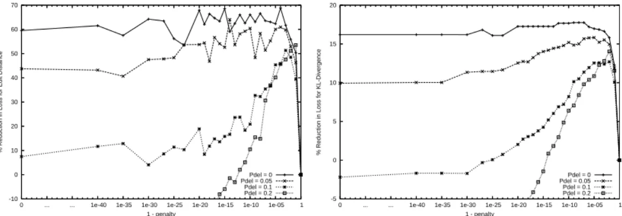
Figure 2.2: Reduction in edit distance (left) and KL-Divergence (right) for ALARM
The ALARM and INSURANCE problems
Figures 2.2 and 2.3 show the average percent reduction in loss, in terms of edit dis-tance and KL-divergence, achieved by multitask learning over single-task learning for a training set of 1000 points on the ALARM and INSURANCE-IND problems. The figures for the ALARM-IND and INSURANCE problems are similar and are not included. On the x-axis we vary the penalty parameter of the multitask prior on a log-scale.7 Note that the x-axis plots 1−penalty. The higher the penalty
(the lower 1−penalty), the more similar the learned structures will be, with all the structures being identical for a penalty of one (1−penalty = 0, left end of graphs). Each line in the figure corresponds to a particular value of Pdel. Error
bars are omitted to maintain the figure readable.
The trends in the graphs are exactly as expected. For all values of Pdel, as the
penalty increases, the performance increases because the learning algorithm takes into account information from the other tasks when deciding whether to add a new arc or not. If the penalty is too high, however, the algorithm loses the ability to find true differences between tasks and the performance drops. As the tasks become more similar (lower values of Pdel), the best performance is obtained at
7
The log-scale is needed because we are working in the probability space so 1−δ needs to
-10 -5 0 5 10 15 20 25
0 ... ... 1e-40 1e-35 1e-30 1e-25 1e-20 1e-15 1e-10 1e-05 1
% Reduction in Loss for Edit Distance
1 - penalty Pdel = 0 Pdel = 0.05 Pdel = 0.1 Pdel = 0.2 -10 -5 0 5 10
0 ... ... 1e-40 1e-35 1e-30 1e-25 1e-20 1e-15 1e-10 1e-05 1
% Reduction in Loss for KL-Divergence
1 - penalty
Pdel = 0 Pdel = 0.05 Pdel = 0.1 Pdel = 0.2
Figure 2.3: Reduction in edit distance (left) and KL-Divergence (right) for INSURANCE-IND
higher penalties. Also as the tasks become more similar, more information can be extracted from the related tasks, so usually multitask learning provides more benefit. As expected, multitask structure learning provides a larger improvement in edit distance than in KL-divergence. This happens because multitask structure learning helps to correctly identify the arcs that encode weaker dependencies (or in-dependences) which have a smaller effect on KL-divergence. The arcs that encode strong dependencies, and have the biggest effect on KL-divergence, can be easily learned without help from the other tasks. multitask learning provides similar ben-efits whether the tasks have highly correlated parameters (ALARM and INSUR-ANCE problems) or independent parameters (ALARM-IND and INSURINSUR-ANCE- INSURANCE-IND problems). This shows that making the parameters independenta priori (see Section 2.3) does not hurt the performance of multitask learning. However, if we were able to take advantage of the similarity between the parameters of the different tasks, we could presumably improve performance even further.
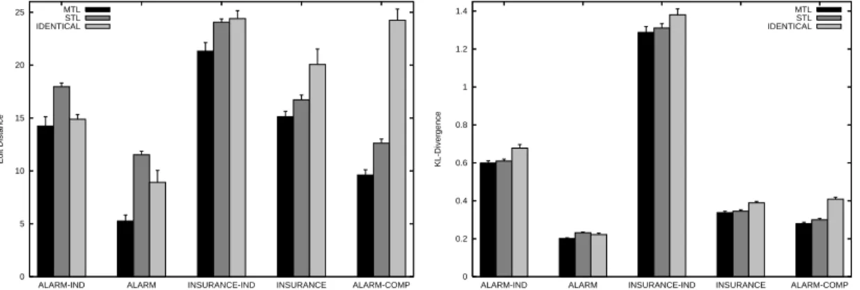
Figure 2.4 shows the edit distance (left) and KL-divergence (right) performance of multitask structure learning when using the different multitask priors proposed in Section 2.3.1: the Paired prior from equation 2.8 with the reversed edges penal-ized twice (Paired/Double) or only once (Paired/Single) and the Edit prior from
0 5 10 15 20 25
ALARM-IND ALARM INSURANCE-IND INSURANCE ALARM-COMP
Edit Distance Paired/Double Paired/Single Edit 0 0.2 0.4 0.6 0.8 1 1.2 1.4
ALARM-IND ALARM INSURANCE-IND INSURANCE ALARM-COMP
KL-Divergence
Paired/Double Paired/Single Edit
Figure 2.4: Edit distance (left) and KL-Div (right) for different multitask priors
0 5 10 15 20 25
ALARM-IND ALARM INSURANCE-IND INSURANCE ALARM-COMP
Edit Distance MTL STL IDENTICAL 0 0.2 0.4 0.6 0.8 1 1.2 1.4 ALARM-COMP INSURANCE INSURANCE-IND ALARM ALARM-IND KL-Divergence MTL STL IDENTICAL
Figure 2.5: Edit distance (left) and KL-Div (right) for STL, learning identical structures and MTL
equation 2.7. Each group of bars corresponds to one problem. For ALARM-IND, ALARM, INSURANCE-IND and INSURANCE Pdel is set to 0.05. The training
set has 1000 cases, with a validation set of 50 cases for selecting the penalty pa-rameter for the multitask prior as described in the beginning of this section. While there is some variability between the performance of the different priors, it is quite small, and never statistically significant. This suggests that multitask learning is relatively robust to the specific type of multitask prior, as long as it appropriately encourages sharing between the tasks. So one can safely use either type of prior without having to worry about selecting the best prior for the problem. Unless otherwise specified, in his chapter we use the Paired prior with double penalty on reversed edges.
Figure 2.5 shows the edit distance and KL-Divergence performance for single task learning (STL), learning identical networks via the algorithm presented in Section 2.3.1 (IDENTICAL), and multitask learning (MTL) for the five problems. The training set has 1000 instances with 50 instances used to select the penalty parameter for the multitask prior. Single-task learning and identical structure learning use both the training and the validation data to learn both the structure and the parameters of the Bayes Nets. The figure shows that multitask learn-ing yields a 10%-54% reduction in edit distance and a 2% - 13% reduction in KL-divergence when compared to single task structure learning. All differences except for KL-divergence on ALARM-IND and INSURANCE-IND problems are .95 significant according to paired T-tests. When compared to learning identical structures, multitask learning reduces the KL-divergence 7% - 32% and the num-ber of incorrect arcs in the learned structures by 4% - 60%. All differences are .95 significant, except for edit distance on the ALARM-IND problem. Since the five tasks for the ALARM, INSURANCE, and ALARM-COMP problems share a large number of their parameters, simply pooling the data might work well. However, this is not the case. Except for the ALARM problem, where it achieves about the same edit distance as learning identical structures, pooling the data has much worse performance both in terms of edit distance and in terms of KL-divergence.
For a qualitative perspective, Figure 2.6 shows the true structures and the structures learned by multitask learning and single-task learning for the five tasks (one per row) on one trial of the ALARM-COMP problem. The figure clearly shows that multitask learning finds more accurate structures by taking advantage of the similarity between the five tasks, while still preserving some of the true differences between them.
1 2 4 7 3 5 6 36 8 28 9 15 16 22 33 35 10 11 14 12 13 32 17 20 26 18 19 23 21 34 24 25 37 27 30 31 29 1 2 4 7 3 5 6 36 8 28 9 15 22 33 35 10 11 14 12 13 16 32 17 20 26 18 19 23 21 34 24 25 37 27 30 31 29 1 2 7 19 29 3 4 6 5 36 8 28 9 22 33 35 10 11 14 12 13 16 15 32 17 20 26 18 23 21 34 24 25 37 27 30 31 1 4 5 2 3 6 7 36 8 28 9 15 16 22 33 35 10 11 14 12 13 32 17 20 26 18 19 23 21 34 24 25 37 27 30 31 29 1 2 5 3 4 6 7 36 8 28 9 15 16 22 33 35 10 11 12 13 14 32 17 20 26 18 19 23 21 34 24 25 37 27 30 31 29 1 5 2 3 4 6 7 36 8 11 28 9 22 34 35 10 19 13 12 14 16 15 32 17 20 33 26 18 23 21 24 25 37 27 30 31 29 1 2 4 7 3 5 6 36 8 28 9 15 16 22 33 35 10 13 11 12 14 21 34 32 17 20 26 18 19 23 24 25 37 27 30 31 29 1 2 4 3 5 6 7 36 8 28 9 15 22 35 10 13 16 33 11 12 14 34 32 17 20 26 18 19 23 21 24 25 37 27 30 31 29 1 4 5 7 2 3 6 36 8 28 9 15 22 35 10 13 16 33 11 12 14 34 32 17 20 26 18 19 27 23 21 24 25 37 30 31 29 1 2 4 7 3 5 6 36 8 30 9 15 16 22 33 35 10 11 14 12 13 32 17 20 26 18 19 23 21 34 24 25 37 27 28 31 29 1 2 4 3 5 6 7 8 9 15 22 33 35 10 11 12 13 14 32 16 17 20 26 18 19 23 21 34 24 25 37 27 29 28 30 31 36 1 2 4 7 3 24 5 6 8 9 15 22 35 10 11 13 21 12 14 32 16 17 20 26 18 19 23 34 25 37 27 28 29 30 31 33 36 1 4 5 2 3 6 7 36 8 30 9 15 16 22 33 35 10 11 14 12 13 32 17 20 26 18 19 23 21 34 24 25 37 27 28 31 29 1 2 4 5 3 6 7 8 9 15 22 33 35 10 11 12 13 14 32 16 17 20 26 18 19 23 21 34 24 25 37 27 29 28 31 30 36 1 4 2 3 5 6 7 8 9 22 35 10 11 18 12 13 14 15 32 33 16 20 17 26 21 19 23 24 25 37 27 28 31 29 30 34 36
Figure 2.6: The true structures (left), structures learned by MTL (middle) and STL (right) for ALARM-COMP
TRUE STRUCTURE MTL STL T AS K 1 T AS K 2 T AS K 3 T AS K 4 T AS K 5
0 5 10 15 20 25 30 250 500 1000 2000 4000 8000 16000 Edit Distance
Training Set Size
STL MTL 0 0.2 0.4 0.6 0.8 1 1.2 250 500 1000 2000 4000 8000 16000 KL-Divergence
Training Set Size
STL MTL
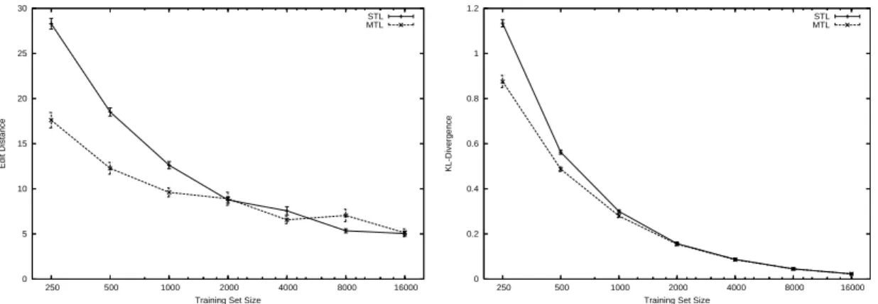
Figure 2.7: Edit distance (left) and KL-Divergence (right) vs. train set size for ALARM-COMP.
set size varies from 250 to 16000 cases (MTL uses 5% of the training points as a validation set to select the penalty parameter). As expected, the benefit from multitask learning is larger when the data is scarce and it diminishes as more training data is available. This is consistent with the behavior of multitask learning in other learning setting (see e.g. (Caruana, 1997)). For smaller training set sizes multitask learning needs about half as much data as single-task learning to achieve the same edit distance. In terms of KL-divergence, multitask learning provides smaller savings in sample size. One reason for this is that, as discussed before, multitask learning yields lower improvements in KL-divergence than in edit distance. For the most part however, the smaller savings in sample size are due to the fact that more training data leads not only to more accurate structures, but also to more accurate parameters. Since multitask structure learning only improves the structure and not the parameters, it is not able to make up for the loss of large amounts of training data.
The BIRD problem
The results on the BIRD problem mimic the ones in the previous section. Fig-ure 2.8 shows the average (across the 6 BCRs/tasks) mean log likelihood on a large independent test set for multitask structure learning as a function of the penalty
-40.42 -40.4 -40.38 -40.36 -40.34 -40.32 -40.3 -40.28 -40.26 -40.24 -40.22
0 ... ... 1e-40 1e-35 1e-30 1e-25 1e-20 1e-15 1e-10 1e-05 1
Mean Log Likelihood
1 - penalty
Paried/Double Edit
Figure 2.8: Average mean log likelihood vs. the penalty parameter for multitask structure learning on the BIRD problem.
parameter of the multitask prior. Each line corresponds to a different type of mul-titask prior. The x-axis plots 1−penalty, so the right most point corresponds to no penalty (single task learning) and the leftmost point corresponds to a penalty of one (learning identical structures). Higher mean log likelihood represents bet-ter performance. As with the five problems in the previous section, the type of multitask prior does not have a significant impact on the performance of multitask learning. As the penalty parameter increases (1−penalty decreases), information starts to be transfered between the different tasks and the performance quickly increases. After reaching a peak, the performance starts to decrease slowly as the penalty increases further.
Note that, because the tasks are not all defined on the same set of variables (see Section 2.3.4), the algorithm for learning identical structures for all tasks from Section 2.3.1 can not be directly applied. Our algorithm on the other hand can handle this situation and learns a set of identical structures for all tasks that performs reasonably well (left end of Figure 2.8).
Figure 2.9 shows the average mean log likelihood performance of multitask structure learning and single task structure learning as a function of the training set size. multitask learning uses 5% of the training data to select the penalty
pa--41.8 -41.6 -41.4 -41.2 -41 -40.8 -40.6 -40.4 -40.2 -40 -39.8 -39.6 250 500 750 1000
Mean Log Likelihood
Training Set Size
STL MTL
Figure 2.9: Average mean log likelihood vs. training set size for the BIRD problem. rameter for the multitask prior. As with the other problems, the benefit from mul-titask learning is larger for smaller training set sizes. As the training size increases single-task learning catches up and eventually outperforms multitask learning. Un-fortunately, since we do not know the real network structures for this problem, we can not directly asses the quality of the learned structures. The results in the previous sections, however, suggest that if one would be able to measure the edit distance between the true and the learned structures, the improvement provided by multitask learning in terms of edit distance probably would be even larger than the improvement provided in terms of average mean log likelihood.
2.4
Task Selection for Multitask Structure Learning
In any multitask learning setting there is a trade-off between correct transfer of features that are truly common between tasks, and incorrect transfer of features that in reality are distinct. More correct transfer translates into more benefit from multitask learning while incorrect transfer diminishes or even eliminates this benefit.
In multitask structure learning this trade-off is controlled via the multitask prior. If the tasks are closely related (i.e. their true structures are very similar)
then there is less opportunity for incorrect transfer and the multitask prior can safely encourage more sharing between tasks leading to higher benefits. Conversely, if the tasks are more dissimilar then incorrect transfer becomes more of a concern and the sharing between tasks needs to be toned down. The problem arises when some of the tasks are closely related, but others are quite dissimilar. In this case, multitask structures learning is either forced to lower the sharing between tasks and miss some opportunities for correct transfer from the closely related tasks, or to suffer from incorrect transfer from the dissimilar tasks. In both cases, the performance of multitask structure learning will be lower than if it were to only use the closely related tasks.
In what follows, we slightly change the problem setup, and assume that there is a singleprincipal task that we are interested in learning a good network structure for. If more than one task is important, then the procedure can be repeated with each important task as the principal task. We also assume that there exists a pool of potentially related extra tasks, but we are not interested in their network structures. Under these assumptions, the goal of task selection is to find a set of tasks that, when used as extra tasks in multitask structure learning, maximize the performance of the principal task.
As discussed above, the more related a task is to the principal task, the higher the benefit it provides. This justifies the following task selection procedure: first order all the extra tasks by a measure of their relatedness to a principal task, then select the first (most related) N tasks to use as related tasks. N, the number of tasks to be selected, can either be specified by the user, or selected using an independent validation set.
This task selection procedure relies on having a measure of task relatedness. In the rest of the section we propose two such task relatedness measures.
2.4.1
A Direct Measure of Task Relatedness
Unlike most multitask learning settings, where the notion of task relatedness is not well defined, in the multitask structure learning setting there is a clear definition of relatedness: two tasks are related if they have similar structures. So any measure of similarity/dissimilarity between the true Bayes Net structures of two tasks provides a direct measure of the similarity/dissimilarity between the two tasks.
Since the true network structures are not available, we need to approximate the similarity between two tasks without having access to the true structures them-selves. A simple way to do this is to first learn the network structures for each task from the training data (in a single-task manner), then use the learned net-works to compute the similarity between the different tasks. One potential problem with this approach is that the greedy search procedure used to learn the network structures is a high variance procedure. This variance might make the learned networks artificially dissimilar leading to a poor, high variance, approximation of the similarity between different tasks.
This problem can be alleviated by encouraging the greedy search procedure to follow similar search paths for all task. Luckily, multitask structure learning does just that: it gives greedy search an incentive to make similar decisions for every task, making the search paths for all tasks similar. This incentive, quantified by the penalty parameter of the multitask prior, should be large enough to cut down the variance, but small enough not to make the learned structures artificially similar. In our experiments using a penalty parameter of 0.9 worked well.
To put it all together, the procedure we propose for measuring task relatedness consists of the following two steps:
1. Learn the structures for all the tasks using multitask structure learning with a small penalty parameter.
2. For each pair of tasks, use the similarity between their learned structures as a measure of similarity between the two tasks.
Note that the multitask structure learning at step 1 is only used as a pre-processing step. The structures learned are used only to compute the similarity between the tasks.
The measure of structure similarity/dissimilarity that is used to evaluate the task relatedness should reflect, if possible, the same prior beliefs about how the structures should be shared that are encoded in the multitask structure learning prior. For example if the prior belief is that part of the network structure should not be shared (e.g. the prior in Section 2.3 have a penalty of 0 for some of the arcs) then the similarity/dissimilarity measure should also ignore the respective part of the structure. In our experiments, we used the edit distance between two structures as a measure of dissimilarity between structures.
An added bonus of this method of assessing task relatedness is that it generates a proper distance metric between tasks. This is a desired property, especially if one wants to cluster the tasks rather than just order them.
2.4.2
An Indirect Measure of Task Relatedness
Another measure of task relatedness can be obtained using the following procedure: 1. Learn the structure of the first task using only data from the first task. 2. Keeping the structure fixed, learn the parameters using only data from the
second task.
3. Compute the mean log likelihood of an independent validation set from the second task.
Steps 2 and 3 can of course be replaced with a cross-validation procedure in order to obtain a more accurate estimate of the mean log likelihood performance. In our experiments we use ten-fold cross validation, and use the average mean log likelihood over the ten folds as a measure of task relatedness.
This task relatedness measure is based on the intuition that the more related the tasks are, the more the network structure of one task should be compatible with the other task leading to a better mean log likelihood. Measuring task relatedness this way however, has a number of disadvantages when compared to the direct measure proposed in the previous section: it does not measure quite the right thing, it is not a metric (it is not even symmetric) and it can not be adapted to reflect different prior beliefs about how the structures should be shared.
2.4.3
Empirical Evaluation
We test the task selection method using a variation of the ALARM-COMP prob-lem, and the bird ecology data.
Given the number of tasks to be selected, N, we evaluate the performance of multitask structure learning with task selection using the following procedure:
1. Compute the similarity between each extra task and the principal task. 2. Select the most similar N tasks to use as related tasks.
3. Learn the network structure of the principal task and the N selected tasks using multitask structure learning.
4. Report the Edit Distance and KL-Divergence between the learned network and the true network for the principal task.
0.2 0.21 0.22 0.23 0.24 0.25 0.26 0.27 1 2 3 4 5 6 7 8 9 10 11 12 13 14 15 16 KL-Divergence
Number of Selected Tasks
DIRECT INDIRECT TRUE DIRECT, Optimal Penalty INDIRECT, Optimal Penalty TRUE, Optimal Penalty
Figure 2.10: KL-Divergence of the principal task vs. the number of selected tasks for the ALARM-COMP problem.
The ALARM-COMP problem
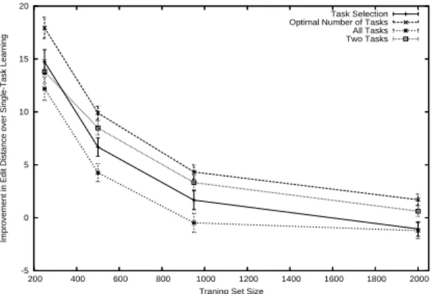
As a first test, we attempt to recover the structure of the original ALARM network. The pool of extra tasks consist of all fifteen tasks that can be generated using the ALARM-COMP method described in Section 2.3.4: four tasks where only one of the four components is changed, six tasks where two components are changed, four tasks where three components are changed, and one task where every component is changed. Note that the arcs between components are never changed (they are the same as in the original ALARM network), so all the extra tasks have some degree of similarity to the principal task. All results in this section are averages across fifty random trials.
Figure 2.10 shows the KL-Divergence between the true and the learned net-works for the principal task (the original ALARM network) as N, the number of tasks to be selected by the task selection procedure, varies from 0 (single task learning) to 15 (no task selection) for a training set of 1000 points. The two groups of lines in the graph show the performance when the penalty parameter for the multitask prior is selected using a small validation set of 50 points (the upper group), and when the penalty parameter is selected optimally (the lower group). Each group has three lines corresponding to three different measure of task