Resolution of Defaulted Loan Contracts
An Empirical Analysis of Default Resolution Time
and Loss Given Default
Jennifer Betz
Center of Finance
Faculty of Business, Economics, and Management Information Systems
An Empirical Analysis of Default Resolution Time
and Loss Given Default
A dissertation in partial fulfillment of the requirements for the degree of Doktor der Wirtschaftswissenschaft (Dr. rer. pol.)
submitted to the
Faculty of Business, Economics, and Management Information Systems
University Regensburg
submitted by
Jennifer Betz
, M.Sc. in Business AdministrationAdvisors
Prof. Dr. Daniel R ¨osch
Prof. Dr. Gregor Dorfleitner
Date of disputation July, 11th 2018
First and foremost, I would like to express my true gratitude to Prof. Dr. Daniel R¨osch for his continuous support, his huge enthusiasm, and unending patience. I would like to thank him for always having an open door and for being the most encouraging supervisor I could ever imagine. It is a tremendous privilege and pleasure to have him as my first advisor. I am grateful to Prof. Dr. Gregor Dorfleitner for being my second advisor. Furthermore, I would like to thank him for raising my enthusiasm in research and for encouraging me to pursue this path.
I am grateful to all of my colleagues for any statistical and non-statistical discussion and, more than anything, for an amazing time. In particular, I would like to thank my two co-authors, Dr. Ralf Kellner and Dr. Steffen Kr ¨uger. Steffen – thank you for one or another lesson in math and for sharing your office with me. Ralf – thank you for your hard deadlines, each and every coffee at math, and for representing an example worth following.
Last but not least, I would like to thank my wonderful family and awesome friends. Above all, I am grateful to Sebastian Ertl for his love, his constant encouragement, and for listening to weird statistical problems in the middle of the night.
I would like to dedicate this thesis to the most wonderful parents in this world, Suzanne and Helmut Betz. All I am, I am because of you. Thank you for your unconditional love, your care, and your continuous support during my entire life. Thank you for teaching me not to quit if goals are worth reaching. Dad – thank you for reminding me to take a break from time to time. Mom – thank you for your eternal belief in me, even in times I have lost it.
Contents
List of Figures v
List of Tables vii
Introduction 1
1 What drives the time to resolution of defaulted bank loans? 9
1.1 Introduction . . . 10
1.2 Data description . . . 12
1.3 Determinants of the TTR . . . 19
1.3.1 General drivers of the TTR . . . 19
1.3.2 Country specific differences . . . 24
1.3.3 Comparison to general drivers of LGD . . . 32
1.4 Robustness . . . 36
1.5 Conclusion . . . 38
1.A Appendix|Log transformation . . . . 40
1.B Appendix|Truncated regression . . . . 44
1.C Appendix|Alternative dependent variable . . . . 47
1.D Appendix|LGD concepts . . . . 49
2 Macroeconomic effects and frailties in the resolution of non-performing loans 50 2.1 Introduction . . . 51
2.2 Why care about systematic effects among DRTs? . . . 54
2.3 Methods and data . . . 58
2.3.1 Methods . . . 58
2.3.2 Data . . . 60
2.4 Results . . . 65
2.4.1 Overview of formal and informal proceedings of resolution . . . 65
2.4.2 Loan specific impacts on resolution . . . 69
2.5 Implications of systematic DRTs . . . 81
2.5.1 Implications on loan level . . . 82
2.5.2 Implications on portfolio level . . . 85
2.6 Conclusion . . . 88
2.A Appendix|Estimation of the Cox model . . . . 90
2.B Appendix|Further analyses . . . . 92
3 Systematic effects among loss given defaults and their implications on downturn estimation 99 3.1 Introduction . . . 100
3.2 Literature review . . . 101
3.3 Background . . . 103
3.4 Methods . . . 104
3.5 Data and results . . . 111
3.5.1 Data . . . 111
3.5.2 Results . . . 116
3.6 Analysis of downturn LGDs . . . 129
3.7 Conclusion . . . 134
3.A Appendix|Bayesian model specification . . . 136
3.B Appendix|Bayesian convergence diagnostics . . . 139
3.C Appendix|Further figures . . . 150
3.D Appendix|Further tables . . . 161
4 Time matters: How default resolution times impact final loss rates 164 4.1 Introduction . . . 165
4.2 Data and methods . . . 168
4.2.1 Data . . . 168
4.2.2 Methods . . . 172
4.3 Empirical results . . . 177
4.4 Validation . . . 185
4.5 Conclusion . . . 190
4.A Appendix|Bayesian model specification . . . 192
4.B Appendix|Bayesian convergence diagnostics . . . 194
Conclusion 204
List of Figures
1.1 Relationship between the TTR and average LGD . . . 14
1.2 Histograms and kernel densities of the TTR . . . 16
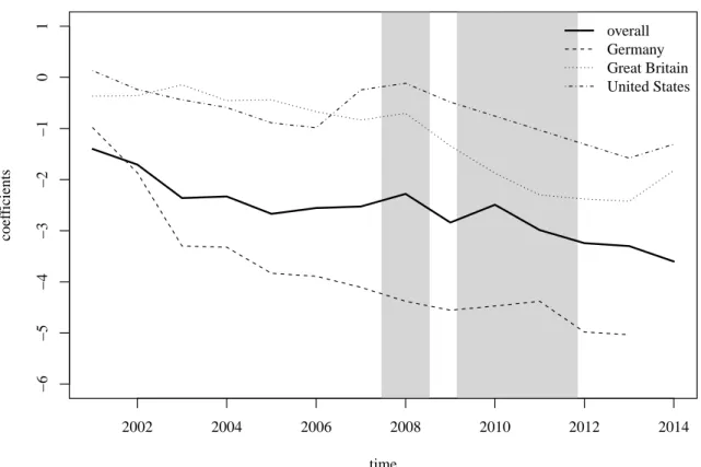
1.3 Progression for the time coefficients in the regression models . . . 29
1.4 Boxplots of LGDs on country level . . . 32
1.A.1 Boxplots of the TTR and its logarithm divided by seniority . . . 42
1.A.2 Boxplots of the TTR and its logarithm divided by collateral . . . 42
1.A.3 Boxplots of the TTR and its logarithm divided by industry . . . 42
2.1 Systematic movements in DRTs . . . 54
2.2 Relation of DRT and non-discounted RR . . . 55
2.3 Additional required amount of stable funding . . . 57
2.4 Resolution time levels . . . 59
2.5 Observed resolution rates . . . 63
2.6 Descriptive statistics of macroeconomic variables . . . 66
2.7 Baseline intensities of resolution . . . 72
2.8 Time-dependent frailties as systematic components of resolution . . . 79
2.9 Relation of DRT and non-discounted RR (representative sample) . . . 82
2.10 Density of DRT . . . 84
2.11 Kernel density estimates of loss on portfolio level . . . 87
2.12 Mean and VaR(95%) of loss on portfolio level . . . 88
2.B.1 Behavior of loan portfolios and default incidence . . . 92
2.B.2 Frailties when including interactions of covariates and recessions . . . 93
2.B.3 Frailty for joint country regression . . . 96
3.1 Histogram and time patterns of LGDs . . . 114
3.2 Random effect in time line (US) . . . 123
3.3 Random effect in time line (GB) . . . 124
3.4 Random effect in time line (Europe) . . . 125
3.6 Posterior and downturn distribution for crises periods based on the macro
model containing the NPL ratio (US) . . . 132
3.7 Downturn distribution for crises periods based on alternative concepts (US) . 133 3.B.1 Trace plots of component model (US) . . . 140
3.B.2 Trace plots of component model (GB) . . . 141
3.B.3 Trace plots of component model (Europe) . . . 142
3.B.4 Trace plots of probability model (US) . . . 145
3.B.5 Trace plots of probability model (GB) . . . 146
3.B.6 Trace plots of probability model (Europe) . . . 147
3.C.1 Exemplary JAGS model file . . . 150
3.C.2 Random effect vs. average LGD . . . 151
3.C.3 Random effect vs. macro variables (US) . . . 152
3.C.4 Random effect vs. macro variables (GB) . . . 153
3.C.5 Random effect vs. macro variables (Europe) . . . 154
3.C.6 Posterior predictive distribution . . . 155
3.C.7 Posterior and downturn distribution for crises periods (GB) . . . 156
3.C.8 Posterior and downturn distribution for crises periods (Europe) . . . 157
3.C.9 Posterior and downturn distribution based on out-of-time estimation . . . 158
3.C.10 Posterior and downturn distribution for crises periods based on the macro model containing the EI (GB) . . . 159
3.C.11 Posterior and downturn distribution for crises periods based on the macro model containing the HPI (Europe) . . . 159
3.C.12 Downturn distribution for crises periods based on alternative concepts (GB) . 160 3.C.13 Downturn distribution for crises periods based on alternative concepts (Europe)160 4.1 Relation of DRT and LGD . . . 169
4.2 Time patterns of average DRTs and average LGDs . . . 171
4.3 Random effect of the LGD model . . . 180
4.4 Random effect of the hierarchical model . . . 184
4.5 Validation (in sample) . . . 187
4.6 Validation (out of sample) . . . 188
4.7 Validation (out of sample out of time) . . . 189
4.8 Validation in the time line . . . 190
4.B.1 Trace plots of the component parameters (LGD model) . . . 195
4.B.3 Trace plots of the covariate parameters and the random effect parameter (LGD model) . . . 197 4.B.4 Trace plots of the component parameters (hierarchical model) . . . 199 4.B.5 Trace plots of the cut points (hierarchical model) . . . 200 4.B.6 Trace plots of the covariate parameters and impact parameter (hierarchical
model) . . . 201 4.B.7 Trace plots of the intercept and covariate parameters (hierarchical model) . . . 202 4.B.8 Trace plots of the standard error and the random effect parameters (hierarchical
1.1 Descriptive statistics . . . 15
1.2 Industry sectors regarding to equity indices . . . 18
1.3 Regression results of the TTR for the overall data set . . . 20
1.4 Insolvency codes in Germany, Great Britain, and the United States . . . 25
1.5 Regression results of the TTR on country level . . . 28
1.6 Determination of . . . 33
1.7 Regression results of the LGD for the overall data set . . . 34
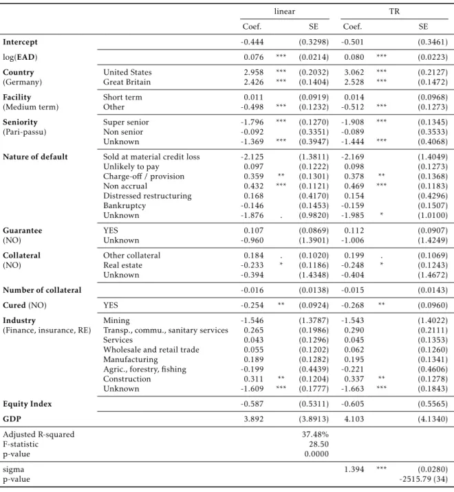
1.A.1 Regression results of the log transformation of the TTR for the overall data set 43 1.B.1 Regression results of the TTR for the linear and the truncated regression (TR) regarding 2008 . . . 45
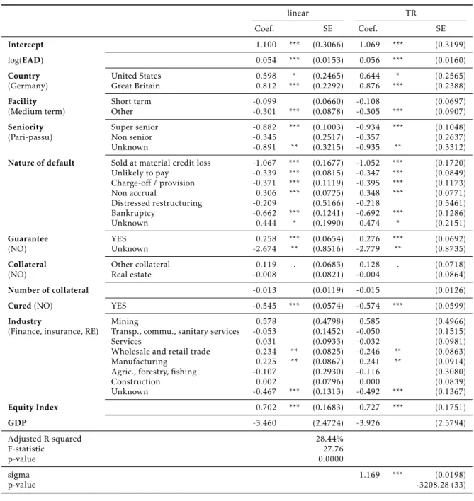
1.B.2 Regression results of the TTR for the linear and the truncated regression (TR) regarding 2009 . . . 46
1.C.1 Regression results of the loan duration for the overall data set . . . 48
1.D.1 GCD transaction types . . . 49
2.1 Descriptive statistics of DRT . . . 62
2.2 Descriptive statistics of loan specific characteristics . . . 64
2.3 Pairwise correlations of macroeconomic variables . . . 65
2.4 Overview of formal and informal proceedings . . . 67
2.5 Regression results for Model I . . . 69
2.6 Regression results for Model II . . . 75
2.7 Regression results for Model III . . . 77
2.8 Frailty impact on mean DRT . . . 78
2.9 Inferences of systematic factors on the distribution of DRTs . . . 84
2.10 Non-discounted RR by DRT buckets . . . 85
2.11 Inferences of systematic factors on the distribution of portfolio DRTs . . . 86
2.B.1 Regression results for Model III when including interactions of covariates and recessions (parameter estimates non-recession) . . . 94
2.B.2 Regression results for Model III when including interactions of covariates and
recessions (interactions to recessions) . . . 95
2.B.3 Regression results for Model I, II and III across countries . . . 97
2.B.4 Regression results for Model II with different macroeconomic variables . . . . 98
3.1 Results of component model . . . 117
3.2 Results of probability model (specification I) . . . 118
3.3 Results of probability model (specification II) . . . 119
3.4 Results of macro models . . . 127
3.B.1 Gelman-Rubin diagnostic of component model . . . 143
3.B.2 Heidelberger-Welch diagnostic of component model . . . 144
3.B.3 Gelman-Rubin diagnostic of probability model . . . 148
3.B.4 Heidelberger-Welch diagnostic of probability model . . . 149
3.D.1 Literature review . . . 161
3.D.2 Composition of European sample . . . 162
3.D.3 Descriptive statistics . . . 162
3.D.4 Pairwise correlations of macro variables and random effect . . . 163
3.D.5 Results of combined models . . . 163
4.1 Descriptive statistics . . . 170
4.2 Estimation sample and validation samples . . . 172
4.3 Results of the LGD model . . . 178
4.4 Results of the hierarchical model . . . 181
4.B.1 Convergence diagnostics of LGD model . . . 194
Motivation and research questions
Financial stability is indispensable for a robust economic system. However, the financial system is exposed to systemic risk. Extensive cascade effects might expand initially financial crises to the entire economic system as in the Global Financial Crisis (GFC). Although causes seem to be limited to the financial sector, effects on the real economy were serve. After the collapse of Lehman Brothers in September 2008, tightened credit conditions in the financial sector transmitted to the real economy. Companies struggled to roll over debt and were confronted with higher interest rates and shorter terms. Campello et al. (2010) suggest that 57% of U.S. American corporations were concerned by tighten credit conditions. Due to limited access to credit markets, smaller companies were severely affected. These corporations are critical for the U.S. American labor market as they employ 40% of the workforce. As consequence, reported unemployment rate increased to 10.1% in October 2009. Combined with the depressed housing and stock markets, household net wealth decreased by 17 trillion USD. In this context, Brian Moynihan (CEO, Bank of America) stated that ”[...] we, as an industry, caused a lot of damage. Never has it been clearer how poor business judgments we have made have affected Main Street.” (see Financial Crisis Inquiry Commission, 2011). In the final report, the Financial Crisis Inquiry Commission concludes that the GFC was avoidable. Inter alia, they mention failures in financial regulation and supervision and malfunctions in the risk management of systemically important banks as causes of the GFC (see Financial Crisis Inquiry Commission, 2011).
As reaction to the crisis, the Basel Committee on Banking Supervision and the Bank of Interna-tional Settlement adapted regulations of capital requirements (Basel II, see Basel Committee on Banking Supervision, 2006) to prevent future crises. These regulations are referred to as
Basel III (see Basel Committee on Banking Supervision, 2010). Just recently, the post-crisis reform was finalized (see Basel Committee on Banking Supervision, 2017). Failures causing crises might not only be found in the regulatory framework but also in the risk management of systemically important banks. Credit risk is the most substantial type of risk for the majority of financial institutions (see European Banking Authority, 2016b). In the advanced Internal Rating Based (IRB) approach of the Basel regulations, banks are permitted to use own empirical models to quantify capital requirements for credit risk. These capital requirements are calculated based on three central credit risk parameters – theProbability of Default(PD), theLoss Given Default(LGD), and theExposure At Default(EAD). While own empirical models for the PD are allowed under the foundation IRB approach, own LGD and EAD estimates are reserved for the advanced IRB approach. Compared to PD modeling (see, e.g., Altman, 1968; Martin, 1977; Campbell et al., 2008; Hilscher and Wilson, 2017; Das et al., 2007; Duffie et al., 2009), the topic of LGD and EAD modeling is rather sparse in academic literature.
This thesis aims to shed light on the topic of LGD modeling. Most of the LGD literature is based onmarket-basedLGDs (see, e.g., Qi and Zhao, 2011; Loterman et al., 2012, for comparative studies). These are calculated as one minus the price of defaulted debt instruments 30 days after default (share to par value). Market-based LGDs are available for traded debt such as bonds. Considering loan contracts, only workoutLGDs are available in most of the cases. Workout LGDs are calculated based on actual recovery cash flows during the resolution process. Thus, characteristics of workout LGDs differ considerably compared to market-based LGDs. First, workout LGDs are shaped by an even more extreme distributional form. Multi-modality seems to be more pronounced and, thus, higher probability masses at the extremes of no loss (LGD = 0) and total loss (LGD = 1) occur. Both modes are shaped by bindings, i.e., LGD values which are exactly zero or exactly one. Second, systematic effects among average LGDs differ due to the underlying process. While market-based LGDs arise at a certain point in time, i.e., 30 days after default, workout LGDs develop over a longer time period – the Time To Resolution(TTR) or Default Resolution Time(DRT).1This hardens the identification of economically and statistically significant (evident) systematic variables, e.g., macro(-economic) variables, as the economic surrounding during the entire resolution process might impact workout LGDs. However, the identification of systematic variables is crucial as LGD predictions are required to reflect economic downturn conditions (see Basel Committee on Banking Supervision, 2006, 2005). Third, workout LGDs are shaped by the resolution bias. Assuming positive dependencies of DRTs and LGDs, bad loan contracts are characterized by long DRTs and high LGDs. These 1 In this thesis, both terms – TTR and DRT – are used as synonyms.
loans are underrepresented at the end of the observation period as only LGDs of loans with short DRTs and, thus, low LGDs, are observable. This might entail parameters distortions and, consequently, an underestimation of LGDs.
Given the characteristics of workout LGDs, the consideration of the resolution process seems to be crucial in the context of defaulted loan contracts. This thesis pursues an comprehensive empirical analysis of the two central parameters of the resolution process – the DRT and the LGD. Hereby, it aims to answer following research questions.
Research question I|What are the drivers of DRTs?
The first paper of this thesis (see Chapter 1,What drives the time to resolution of defaulted bank loans?), aims to answer the question concerning general drivers of DRTs. Loan-specific and macro(-economic) variables are considered as covariates. Positive dependency structures of DRTs and LGDs emphasize the importance of DRTs in credit risk management. Long DRTs are accompanied with higher uncertainty regarding the timing of recovery cash flows. Furthermore, long resolution processes increase liquidity and interest rate risk.
Research question II|How are systematic effects among DRTs?
The second paper of this thesis (see Chapter 2,Macroeconomic effects and frailties in the resolution of non-performing loans), aims to answer the question concerning systematic effects among DRTs. Observable and unobservable systematic factors are considered. Systematic movements in DRTs might imply time-dependent correlation structures, i.e., averagely higher (lower) DRTs at certain points in time. Financial institutions might be able to compensate single defaulted loan contracts with high DRTs, however, correlations might increase the systematic risk of credit portfolios and, thus, further burden liquidity in crises periods.
Research question III|How are systematic effects among LGDs?
The third paper of this thesis (see Chapter 3,Systematic effects among LGDs and their implications on downturn estimation), aims to answer the question concerning systematic effects among LGDs. Following Basel Committee on Banking Supervision (2006, 2005), LGD predictions are required to reflect economic downturn conditions. Thus, the identification of systematic factors is crucial. However, common macro(-economic) variables might not be suited due to the complexity of identifying reasonable observable variables considering workout LGDs.
Unobservable systematic factors in terms of random effects are applied to analyze their ability to generate sufficiently conservative downturn predictions.
Research question IV|How are the dependency structures among DRTs and LGDs?
The forth paper of this thesis (see Chapter 4,Time matters: How default resolution times impact final loss rates), aims to answer the question concerning the dependency structures among DRTs and LGDs. A combined modeling approach is developed to deeply examine the dependence structure among DRTs and LGDs allowing for a direct and an indirect channel. Furthermore, effects of the resolution bias are quantified on an in sample and out of sample perspective comparing a pure (standard) LGD model with the combined modeling approach.
Literature
Although the DRT is crucial considering default resolution and, thus, the LGD, of defaulted loan contracts, most of the literature refers to the resolution of bankruptcy. Furthermore, a majority of publications relate to U.S. data, i.e., the resolution of Chapter 7 and Chapter 11 bankruptcies. Bandopadhyaya (1994) applies a hazard rate model to analyze the time spend under Chapter 11, whereas, Helwege (1999) uses Ordinary Least Square (OLS) regression to examine borrower specific influences on the DRT. Bris et al. (2006) run OLS and Heckman models to compare Chapter 7 and Chapter 11 resolutions. Partington et al. (2001), Denis and Rodgers (2007), and Wong et al. (2007) apply survival analysis.2
In contrast, the literature on LGD modeling has widened considerably in the last decades (see, e.g., Qi and Zhao, 2011; Loterman et al., 2012, for comparative studies). Given the demand for LGD predictions which reflect economic downturn conditions (see Basel Committee on Banking Supervision, 2006, 2005), the identification of systematic variables is crucial in an LGD modeling context. A common tool to consider systematic effects are observable, i.e., macro(-economic), variables. However, the identification of economically and statistically significant (evident) variables is ambiguous. Thus, some authors completely neglect systematic variables (see Bastos, 2010; Bijak and Thomas, 2015; Calabrese, 2014; G ¨urtler and Hibbeln, 2013; Matuszyk et al., 2010; Somers and Whittaker, 2007). In other publications, univariate significance (evidence) can not be confirmed in a multivariate context (see Acharya et al., 2007; Brumma et al., 2014; Caselli et al., 2008; Dermine and Neto de Carvalho, 2006; Grunert and Weber, 2009). Reasons might be found in non-linear impacts of observable systematic variables on LGDs. Acharya et al. 2 A comprehensive literature review regarding the DRT can be found in Chapter 1 (Section 1.1, Introduction) and
(2007) find statistical significance of industry distress dummies, but not for continuous variables. Using quantile regression techniques, Kr ¨uger and R¨osch (2017) identify statistically significant macro(-economic) variables on the inner quantiles of the LGD distribution. Again, this can be traced back to non-linear influences. In parts of the literature, statistical significance (evidence) is not reported (see Altman and Kalotay, 2014; Tobback et al., 2014; Yao et al., 2015). Statistical significance (evidence) might be found where data sets of bonds (see Jankowitsch et al., 2014; Nazemi et al., 2017; Qi and Zhao, 2011), credit cards (Bellotti and Crook, 2012; Yao et al., 2017), or mortgages (Leow et al., 2014; Qi and Yang, 2009) are applied. Bond data sets are usually characterized by market-based LGDs, thus, the identification of economically and statistically significant (evident) macro(-economic) variables might be more straightforward as the LGD is not the result of a complex resolution process, but determined 30 days after default occurred. Credit cards and mortgages belong to the bulk businesses of financial institutions. Hence, resolution processes might be standardized to a higher extend compared to corporate loans.3
To the best of my knowledge, no publication exists so far which covers the dependency structures of DRTs and LGDs. However, the importance of DRTs in an LGD modeling context is indicated in the related literature. Dermine and Neto de Carvalho (2006) apply mortality analysis on a data set of defaulted loan contracts, whereas, G ¨urtler and Hibbeln (2013) are, inter alia, concerned with the resolution bias. They suggest to restrict the data set to avoid biased estimates. Chapter 4 (Time matters: How default resolution times impact final loss rates) of this thesis analyzes the possibility to diminish effects of the resolution bias by considering censored observations, i.e., unresolved loan contracts, by a combined modeling approach for DRTs and LGDs. In the credit risk literature, joint modeling approaches are common for PDs and LGDs. Hereby, multivariate random effects are applied to consider time-dependent comovements. (see Bade et al., 2011; R¨osch and Scheule, 2010, 2014)
Contributions
Related to research questions I, II, III, and IV which are stated above, the main contributions of this thesis can be structured by the independent research papers which are presented in the individual chapters of this thesis (see Chapter 1, 2, 3, and 4).
Contribution I|What drives the time to resolution of defaulted bank loans?
Research question I refers to general drivers of the DRT – i.e., the aim of the first research paperWhat drives the time to resolution of defaulted bank loans? is to analyze which loan-specific 3 A comprehensive literature review regarding the LGD can be found in Chapter 3 (Section 3.2, Literature review).
and macro(-economic) variables impact the duration of the resolution process. Using OLS re-gressions, collateralization, seniority, industry, nature of default, and the macro(-economic) environment are identified as important drivers of the DRT. The analysis is conducted for Germany, the United States, and Great Britain. By this means, two major bankruptcy regimes are compared. The German insolvency codes are creditor friendly, whereas, the Anglo-American regulations are rather debtor orientated. The most striking deviations in causalities refer to collateralization and seniority. This can be traced back to the insolvency codes of the considered countries. While the access to collateral in the event of default is straightforward in Germany, it is more complicated in the United States and Great Britain. As consequence, collateralization reduces the DRT to a higher degree in Germany. Creditors seem to be aware of this divergence and seek for the best security mechanism in the limits set by local insolvency codes. Thus, collateralization appears to be more common in Germany, while Anglo-American creditors demand higher ranks in the seniority order.
By the inclusion of year fixed effects, first indications of time-dependent comovement in DRTs arise. Average DRTs seem to be higher (lower) during downturns (upturns). This is also true considering the LGD as dependent variable. Furthermore, LGDs are driven by similar variables, particularly, collateralization and macro(-economic) variables. Significant year fixed effects indicate similar time patterns in LGDs compared to DRTs.
Contribution II|Macroeconomic effects and frailties in the resolution of non-performing loans
Research question II refers to systematic effects among DRTs. As first indications of time-dependent comovement in DRTs arise (seeContribution Ior Chapter 1), the second research paperMacroeconomic effects and frailties in the resolution of non-performing loansaims to analyze systematic effects among DRTs in more detail. Using Cox Proportional Hazard (PH) regressions, three model specifications are compared. In the first specification (model I), loan-specific vari-ables are applied to explain cross-sectional variation in DRTs. The second specification (model II) additionally includes observable systematic effects, i.e., macro(-economic) variables, to account for time-dependent variations. In the third specification (model III), unobservable system-atic effects, i.e., frailty effects, are introduced. These unobservable systematic effects seem to impact DRTs to a rather high extend even after controlling for common loan-specific and macro(-economic) variables. Stated differently, DRTs seem to be clustered in the time line. Economic consequences of clustered DRTs might be considerable. First, the liquidity of financial institutions is burdened in downturn periods as DRTs are systematically longer. Aside from
the direct availability of liquidity, the implementation of the Net Stable Funding Ratio (NSFR), where additional medium and long term liquidity is demanded for certain facilities, e.g., non-performing loans (see Board of Governors of the Federal Reserve System, 2016), adds additional pressure on the liquidity of financial institutions. Second, portfolio loss distributions of non-performing loan contracts are affected by clustered DRTs. Due to dependency structures of DRTs and LGDs, systematic patterns in DRTs are transfered to the loss side. The portfolio loss distribution is shifted towards higher values in downturn periods. Furthermore, the range of the distribution is broadened independent of the economic surrounding. This indicates that expected portfolio losses rise in downturns, while unexpected losses are constantly increased.
Contribution III|Systematic effects among LGDs and their implications on downturn estimation
Research question III refers to systematic effects among LGDs. Observable and, in particular, unobservable systematic effects have considerable impacts on DRTs (see Contribution IIor Chapter 2). Thus, LGDs might be shaped by time-dependent comovements. This is of high relevance considering the demand for LGD predictions which reflect economic downturn conditions (see Basel Committee on Banking Supervision, 2006, 2005). Using a Bayesian Finite Mixture Model (FMM) with a probabilistic substructure, LGD distributions depending on covariates are estimated in the third research paper Systematic effects among LGDs and their implications on downturn estimation. Time-dependent random effects are included in the modeling framework to quantify the systematic nature of LGDs. By this means, deviations among the considered regions, i.e., the United States and Europe, arise. While realizations of the random effect seem to origin independently from an identical distribution in the United States, systematic patterns are characterized by cyclical nature expressed by an autoregressive (AR) process in Europe. The realizations of the random effects are compared with time patterns of common macro(-economic) variables. Thereby, considerable discrepancies occur. These deviations are emphasized when macro(-economic) variables are included in the modeling framework as their impacts seem not to be evident or limited regarding their magnitude.
Furthermore, a methodology to generate appropriate downturn estimations based on random effects is suggested and compared to approaches in the literature. The most common approach refers to the use of macro(-economic) variables in the modeling framework. Due to the limited evidence and magnitude, downturn estimates based on macro(-economic) variables seem to underestimate the probability mass of high losses, while the suggested methodology delivers sufficiently conservative estimates. Further approaches proposed by Calabrese (2014) and Bijak and Thomas (2015) tend to be over-conservative.
Contribution IV|Time matters: How default resolution times impact final loss rates
Research question IV refers to dependency structures of DRTs and LGDs. As an interconnection of DRTs and LGDs appears descriptively (seeContribution Ior Chapter 1 andContribution II or Chapter 2), dependencies of the two parameters are conceivable. In the fourth research paper Time matters: How default resolution times impact final loss rates, a joint modeling approach for DRTs and LGDs is developed. Therefor, an Accelerated Failure Time (AFT) model for the DRT is combined with an FMM with probabilistic substructure for the LGD (seeContribution III or Chapter 3). This approach allows for direct and indirect dependencies. To reflect direct dependencies, the DRT is included into the LGD model. Multivariate normally distributed random effects are implemented to display indirect dependencies, i.e., comovements in the time line. Positive dependency structures of DRTs and LGDs arise which are even more pronounced in extreme economic surroundings. In downturns (upturns), DRTs are longer (shorter) which burdens financial market liquidity. Moreover, LGDs are even higher in downturns due to the strengthened dependence.
The dependence of DRTs and LGDs introduces the resolution bias. In more recent time periods, only LGDs of loan contracts with short DRTs are observable. These loans tend to exhibit high LGDs due to the positive dependence. Thus, loans with long DRTs and high LGDs are underrepresented towards the end of the observation period. Applying a pure (standard) LGD model causes parameter distortions and, consequently, an underestimation of average LGDs on an out of sample perspective. Effects of the resolution bias are diminished by the combined approach. Thus, LGD predictions are adequate on an out of sample perspective.
Structure
This thesis consists of four independent research papers with varying co-authors.4 Chapter 1 presents the first paper (What drives the time to resolution of defaulted bank loans?). The second paper (Macroeconomic effects and frailties in the resolution of non-performing loans) is subject to Chapter 2. In Chapter 3, the third paper (Systematic effects among LGDs and their implications on downturn estimation) is propound. The fourth and last paper (Time matters: How default resolution times impact final loss rates) is comprised in Chapter 4. The Conclusion summarizes, discusses, and provides an outlook.
What drives the time to resolution
of defaulted bank loans?
This chapter is joint work with Ralf Kellner*and Daniel R¨osch†published as:
Betz, J., R. Kellner, D. R¨osch (2016). What drives the time to resolution of defaulted bank loans?Finance Research Letters 18, 7–31.
https://doi.org/10.1016/j.frl.2016.03.013
Abstract
Using a unique data base of Global Credit Data with individual loan information from small and medium sized entities in Germany, Great Britain and the United States, we evaluate the time to resolution of defaulted loans. A comparison across countries reveals country specific drivers for the resolution time which can be explained fairly well by differences in the regulatory and legal framework. Lenders seem to be aware of these differences and adjust their lending behavior in the limits set by these bankruptcy systems of the countries.
Keywords: credit risk; bankruptcy; resolution of financial distress; time to resolution; resolution bias
JEL classification: C51, G01, G28
* University Regensburg, Chair of Statistics and Risk Management, 93040 Regensburg, Germany,
email:[email protected].
† University Regensburg, Chair of Statistics and Risk Management, 93040 Regensburg, Germany,
1.1
Introduction
The time to resolution (TTR) of defaulted loan contracts is of great relevance to all kinds of creditors. Following Hotchkiss et al. (2008), indirect costs – e.g. opportunity costs and reputational losses – are characterized by a considerable magnitude and importance. However, these cost are not directly captured in the loss rate. As they are challenging to measure, the TTR might serve as a proxy (see, e.g., Franks and Torous, 1989; Bris et al., 2006; Annabi et al., 2012). Furthermore, the TTR seems to be positively correlated with the loss given default (LGD) of loan contracts. High TTRs increase uncertainty regarding the timing of cash flows during resolution and, therefore, liquidity and interest rate risk. To the best of our knowledge, no analysis exists so far which deeply examines drivers for the TTR on a transnational basis even though a profound understanding of it seems crucial in an international setting. A reason for missing studies in this field of literature might be found in the lack of data availability. Thus, our paper uses access to a unique loss database provided by Global Credit Data (GCD)1and conducts a detailed and comprehensive analysis of the TTR across Germany, Great Britain, and the United States. We provide insights which components of loans contribute to a short TTR and to which extent it depends on external factors such as the macroeconomic environment. Thereby, substantial differences among Germany, Great Britain, and the United States arise. These might be ascribed to discrepancies in the insolvency regimes.
While there exists a variety of analyses which examine drivers and estimation methods for the loss rate (see, e.g., Grunert and Weber, 2009; Qi and Yang, 2009; Bastos, 2010; Qi and Zhao, 2011; Loterman et al., 2012), the literature regarding the TTR is more limited even though its importance is indicated in the related analyses. Using a database from a Portuguese bank, Dermine and Neto de Carvalho (2006) analyze recovery rates (RRs) by means of survival time analysis. Their results show the importance of the resolution process as the impact of determinants of RRs change over time. In addition, they point out the importance of the timing of cash flows during the resolution process in the presence of interest rate risk. G ¨urtler and Hibbeln (2013) empirically find LGDs to be positively correlated with the TTR and quicker resolution times for defaulted loans which return back to performance. Davydenko and Franks (2008) detect transnational discrepancies caused by varying legislations with respect to the LGD. This might hold true for the TTR. However, previous analyses are restricted to individual 1 GCD is a non profit initiative which aims to help banks to measure their credit risk by collecting and analyzing
historical loss data. They are formally known as the Pan-European Credit Data Consortium (PECDC). See
countries while data sets are usually specific regarding their origin, i.e, banks or courts. Most studies consider the bankruptcy system in the United States – in particular Chapter 11. Helwege (1999) analyzes the TTR of junk bonds using ordinary-least-square (OLS) regressions. In contrast to our analysis, he focuses on borrower specific characteristics and uses a bankruptcy portfolio of minor debtor quality. Bris et al. (2006) use a data set of bankruptcies in Arizona and New York. They run OLS and Heckman models with the log transformation of the TTR as dependent variable and find that the outcome of bankruptcy (reorganization vs. liquidation) has no influence on the TTR. Denis and Rodgers (2007) and Wong et al. (2007) apply survival methods for examining the TTR of Chapter 11 bankruptcies. Overall they detect firm size, pre-default performance and the macroeconomic environment to be important drivers for TTR while accounting information seems to be less relevant. Few analyses have been made with respect to the TTR in other countries. Focusing on Portugal, the main interest of Bonfim et al. (2012) is on access to credit after default. They find that large firms tend to have shorter TTR. This contradicts with results in the United States from Denis and Rodgers (2007) and indicates country specific differences regarding the TTR. Dewaelheyns and Van Hulle (2009) examine bankruptcies in Belgium and observe that, among others, secured debt and industry conditions play an important role for the TTR. However, non of these analyses examine transnational differences with respect to the TTR.
Hence, we try to fill this gap and contribute to the literature in three ways. First, we investigate important drivers for the TTR of loan contracts using a database containing loans of small and medium sized entities (SMEs) from Germany, Great Britain, and the United States. Thereby, we cover two major bankruptcy regimes, i.e., Germany being traditionally creditor friendly and the Anglo American area more debtor orientated. In a second step, we examine whether deviations in the insolvency codes impact the determinants of the TTR on an inner-country basis and, thus, whether adjustments of lending regularities arise. This approach is motivated by Davydenko and Franks (2008) who show how differences in creditors’ rights impact the general lending behavior in France, Germany, and the United Kingdom. Third, we analyze effects of the macroeconomic environment on the TTR. By including defaults from 2000 until 2014, our analysis covers at least one complete economic cycle.
After controlling for explanatory variables, we find that the resolution process in Germany is shortest compared to Great Britain and the United States. The TTR of American (British) loan contracts is c.p. on average 0.1 (0.5) years longer. This is in line with a higher degree of efficiency regarding the resolution of insolvency in Germany that is assigned by the World Bank.
For the overall dataset, we find seniority, nature of default, collateralization, industry, and the macroeconomic environment to be important determinants for the TTR. Additionally, we exam-ine significant differences across countries. The most important results refer to collateralization and its impact on the seniority order. This seems to be driven by varying regulations regarding access to collateral during resolution and the importance of the seniority order during the bankruptcy proceeding given a certain access to collateral. Assuming easy access to collateral during resolution, its existence should reduce the TTR. In Germany,real estatebacked loans as well as loans secured byother collateraltypes are resolved faster by 0.1 and 0.2 years, respectively. The access to collateral seems to be more complicated in the Anglo American counties asother collateralenhances TTR by 0.1 years andreal estateis insignificant in the United States.
It seems that creditors are aware of these country specific features as they seek for the best safety mechanism in the limits set by the insolvency code by adjusting their lending behavior. As the access to collateral is easier in Germany compared to Great Britain and the United States, a majority of German loans is collateralized (72% general, 53%real estate). On the contrary, collateralization in Great Britain (67% general, 42%real estate) and the United States (64% general, 12%real estate) is less usual. Creditors in the Anglo American area seem to compensate this by demanding the highest rank in the seniority order (super senior). In Great Britain (44%) and the United States (84%), a higher fraction of loans exhibit thesuper senior status while German creditors do not depend on being the one and only preferred claimant (5%super senior). This seems to work for creditors in Great Britain as thesuper seniorstatus reduces TTR by 1.2 years. In the United States it suffices to be among preferred claimants as no significant difference regarding TTR occurs among situations with one single and more than one (pari-passu) preferred claimants. However, being not among preferred claimants increases the TTR by 1.4 years.
The remainder of this paper is structured as follows. Section 1.2 provides the data description and descriptive statistics. Section 1.3 presents our main analysis. Section 1.4 provides several robustness tests. Section 1.5 concludes.
1.2
Data description
Our data set consists of a subsample of the unique loss data base composed by GCD. The data base contains historical loss data from 44 member banks. In this paper, we analyze loans of SMEs whose jurisdiction is located in Germany, Great Britain, and the United States. We
focus on these countries as they represent two major bankruptcy regimes, i.e., Germany being traditionally creditor friendly and the Anglo American countries more debtor orientated. The time span of the entire data base reaches from September 1971 until Juli 2014. To ensure a consistent default definition and, thereby, unbiased estimation results, we refer to the default definition set by the Basel Committee on Banking Supervision (2006). A default occurs if an obligor is ”unlikely to pay” or ”past due more than 90 days on any material credit obligation” (§452).2 Pursuant to Brumma et al. (2014), this definition is implemented since the year 2000 which is why we restrict the time period from 2000 to 2014. Furthermore, we eliminate loans with EADs smaller than 500 EUR to satisfy the materiality threshold of the European Banking Authority (2016a). Despite the reference to borrower level, we apply the rule on loan level as loans of this size seem unreasonable. To correct for minor input errors, we follow H¨ocht and Zagst (2010) and H¨ocht et al. (2011) who developed selection criteria on cash flow basis. We apply this approach with the distinction that we separately consider payments during and after the resolution process. Hence, the first criterion is calculated as the sum of all relevant transactions (including charge-offs) divided by the outstanding amount of the loan. Loans falling below 90% or exceeding 110% are sorted out. To verify post resolution payments, we evolve a second criterion. Thereby, the sum of all post resolution payments is divided by a fictional outstanding amount at the resolution date. The barriers are set to−10% and 110%.
Finally, we eliminate loans with abnormal low and high LGDs (<−50% and>150%).3 A subset
of 24,870 individual loans remains.
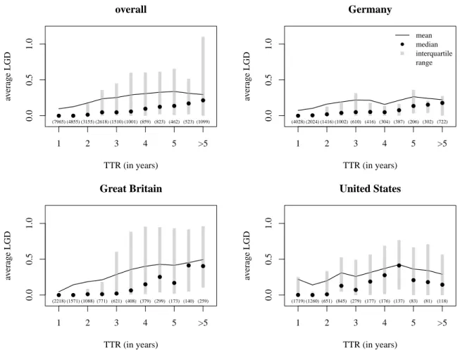
Figure 1.1 shows the relation between the average LGD and the TTR (in years) for the entire data set and the three country subsets. The black lines display the average LGD for the specified TTR buckets. The interquartile ranges are represented by the gray boxes, whereby, the black dots are the medians. The quantity of loans in the buckets is given in brackets. Investigating the general relation of credit losses and the TTR, the upper left panel of Figure 1.1 shows a positive dependence between the average LGD and the TTR in the overall data set. A longer TTR comes along with higher LGDs, and vice versa. The results differ if the same relationship is regarded on country level. While the link between TTR and average LGD seems to increase monotonously in Great Britain, the peak in the United States arises around four and a half years after default occurs. In Germany, a slight drop in the average LGD appears for a TTR of four years.
Figure 1.2 shows histograms and corresponding kernel density estimates of the TTR for the 2 Note that we use default and financial distress in a synonymous way. The data set contains both, loans which are
subject to common resolution mechanisms (e.g., restructuring, liquidation) andcuredloans which returned back to performance after they got into financial distress.
Figure 1.1:Relationship between the TTR and average LGD for the overall dataset and on country level 0.0 0.5 1.0 overall TTR (in years) av erage LGD 1 2 3 4 5 >5 ● ● ● ● ● ● ● ● ● ● ● (7965) (4855) (3155) (2618) (1510) (1001) (859) (823) (462) (523) (1099) 0.0 0.5 1.0 Germany TTR (in years) av erage LGD 1 2 3 4 5 >5 ● ● ● ● ● ● ● ● ● ● ● (4028) (2024) (1416) (1002) (610) (416) (304) (387) (206) (302) (722) ● mean median interquartile range 0.0 0.5 1.0 Great Britain TTR (in years) av erage LGD 1 2 3 4 5 >5 ● ● ● ● ● ● ● ● ● ● ● (2218) (1571) (1088) (771) (621) (408) (379) (299) (173) (140) (259) 0.0 0.5 1.0 United States TTR (in years) av erage LGD 1 2 3 4 5 >5 ● ● ● ● ● ● ● ● ● ● ● (1719) (1260) (651) (845) (279) (177) (176) (137) (83) (81) (118)
Notes: Figure of the average LGD with respect to the resolution time.
overall sample and on country level. The distribution of the TTR is asymmetric and extremely skewed to the right. This indicates that most of the loans exhibit a rather short TTR, but very long resolution times are probable with a certain (small) likelihood. Differences between the countries under investigation can be observed. The overall sample, Germany, and Great Britain show a unimodal distribution while the United States are characterized by bimodality with the second modus around 1.7 years after default.
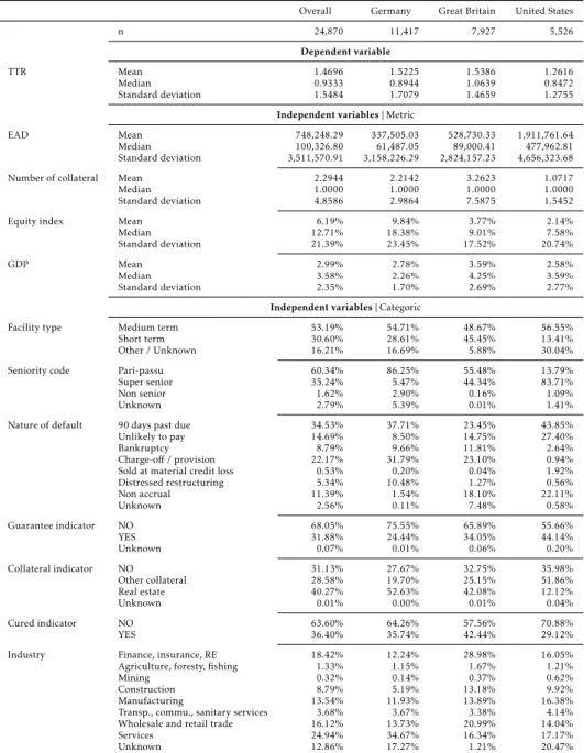
Descriptive statistics of considered quantities for the overall data set and on country level are displayed in Table 1.1. The first row reports the sample size. Most of the 24,870 loans are located in Germany (11,417 loans) followed by Great Britain (7,927 loans) and the United States (5,526 loans). Hence, the overall data set may be dominated by German loans. Furthermore, Table 1.1 contains descriptive statistics regarding dependent and independent variables of the subsequent regression analysis.4 The mean of the TTR is lowest for the United States (1.26 years) followed by Germany (1.52 years) and Great Britain (1.54 years).
Table 1.1:Descriptive statistics for the overall data set and on country level
Overall Germany Great Britain United States
n 24,870 11,417 7,927 5,526
Dependent variable
TTR Mean 1.4696 1.5225 1.5386 1.2616
Median 0.9333 0.8944 1.0639 0.8472 Standard deviation 1.5484 1.7079 1.4659 1.2755
Independent variables|Metric
EAD Mean 748,248.29 337,505.03 528,730.33 1,911,761.64 Median 100,326.80 61,487.05 89,000.41 477,962.81 Standard deviation 3,511,570.91 3,158,226.29 2,824,157.23 4,656,323.68 Number of collateral Mean 2.2944 2.2142 3.2623 1.0717 Median 1.0000 1.0000 1.0000 1.0000 Standard deviation 4.8586 2.9864 7.5875 1.5452 Equity index Mean 6.19% 9.84% 3.77% 2.14% Median 12.71% 18.38% 9.01% 7.58% Standard deviation 21.39% 23.45% 17.52% 20.74%
GDP Mean 2.99% 2.78% 3.59% 2.58%
Median 3.58% 2.26% 4.25% 3.59%
Standard deviation 2.35% 1.70% 2.69% 2.77%
Independent variables|Categoric
Facility type Medium term 53.19% 54.71% 48.67% 56.55% Short term 30.60% 28.61% 45.45% 13.41% Other / Unknown 16.21% 16.69% 5.88% 30.04% Seniority code Pari-passu 60.34% 86.25% 55.48% 13.79% Super senior 35.24% 5.47% 44.34% 83.71% Non senior 1.62% 2.90% 0.16% 1.09% Unknown 2.79% 5.39% 0.01% 1.41% Nature of default 90 days past due 34.53% 37.71% 23.45% 43.85% Unlikely to pay 14.69% 8.50% 14.75% 27.40% Bankruptcy 8.79% 9.66% 11.81% 2.64% Charge-off/ provision 22.17% 31.79% 23.10% 0.94% Sold at material credit loss 0.53% 0.20% 0.04% 1.92% Distressed restructuring 5.34% 10.48% 1.27% 0.56% Non accrual 11.39% 1.54% 18.10% 22.11% Unknown 2.56% 0.11% 7.48% 0.58% Guarantee indicator NO 68.05% 75.55% 65.89% 55.66% YES 31.88% 24.44% 34.05% 44.14% Unknown 0.07% 0.01% 0.06% 0.20% Collateral indicator NO 31.13% 27.67% 32.75% 35.98% Other collateral 28.58% 19.70% 25.15% 51.86% Real estate 40.27% 52.63% 42.08% 12.12% Unknown 0.01% 0.00% 0.01% 0.04% Cured indicator NO 63.60% 64.26% 57.56% 70.88% YES 36.40% 35.74% 42.44% 29.12% Industry Finance, insurance, RE 18.42% 12.24% 28.98% 16.05% Agriculture, foresty, fishing 1.33% 1.15% 1.67% 1.21%
Mining 0.32% 0.14% 0.37% 0.62%
Construction 8.79% 5.19% 13.18% 9.92% Manufacturing 13.54% 11.93% 13.89% 16.38% Transp., commu., sanitary services 3.68% 3.67% 3.38% 4.14% Wholesale and retail trade 16.12% 13.73% 20.99% 14.04% Services 24.94% 34.67% 16.34% 17.17% Unknown 12.86% 17.27% 1.21% 20.47%
Notes: The table contains mean, median, and standard deviation for variables of metric nature and proportions for variables of categoric nature, respectively.
Figure 1.2: Histograms and kernel densities of the TTR for the overall data set and on country level overall TTR (in years) density 0 2 4 6 8 10 12 14 0.0 0.5 1.0 Germany TTR (in years) density 0 2 4 6 8 10 12 14 0.0 0.5 1.0 Great Britain TTR (in years) density 0 2 4 6 8 10 12 14 0.0 0.5 1.0 United States TTR (in years) density 0 2 4 6 8 10 12 14 0.0 0.5 1.0
In Section 1.3, we additionally control for various potential input parameters. Classical metric determinants are the exposure at default (EAD) and macroeconomic variables. We further include the number of collateral as multiple types of collateral can be assigned to a single loan contract. In our data set, loans located in the United States are on average considerably larger (1,911,761.64 EUR) than their counterparts from Great Britain (528,730.33 EUR) and Germany (337,505.03 EUR). The reason for this difference may be found in the heterogeneous ease of getting credit. Since 2004, the World Bank published a score evaluating this topic. Amongst other legal subjects, the seriesDoing Businesscovers – under the sectionGetting Credit– the ease of receiving credit lines (see World Bank, 2015a,b,c,d). Thereby, not only the case of getting credit is analyzed but also its achievable quantity. The score is survey based and expressed as a distance to frontier with 100 representing the optimality. Regarding this score, the United States reaches the second place with a score of 95.00 followed by Great Britain (75.00, 17th place) and Germany (70.00, 24th place). Thus, the access to credit seems to be easier in the United States compared to Great Britain and Germany. The differences in the average EADs might reflect this consideration.
Corresponding to the number of collateral, loans located in Great Britain are on average collateralized with more assets (3.26) than those from Germany (2.21) and the United States (1.07). However, since the median reveals one for all, the majority of loans seems to be secured by a single collateral. To embed macroeconomic variables, several factors were tested with the return of the equity index and of the gross domestic product (GDP) being top of the range regarding the explanatory power in the affiliating analysis.5
In addition, several loan specific categoric variables are included – such as seniority, guarantee, collateral type, and industry indicators. These are also common determinants in modeling LGD (see, e.g., Acharya et al., 2007; Bastos, 2010). It is also controlled for the facility type, nature of default, and if the loan is cured or not, i.e., if the loan returned to performing after being in financial distress.6Table 1.1 displays the shares of the corresponding categories for the overall data set and divided by country. There are solely minor country differences concerning the facility type. Approximately, half of the loans are medium term facilities, whereas the other half is grouped amongst short term and other facilities. Great Britain exhibits the greatest share of short term facilities in the data set (45.45%). Loans located in Germany and the United States are characterized trough a slightly higher proportion in other facilities.
Regarding the seniority code,pari-passuis the prevailing type in the overall data set as well as in Germany (86.25%) and Great Britain (55.48%). In contrast, loans from the United States are mainlysuper senior(83.71%) and only a small fraction (13.79%) appears to bepari-passu.7 With respect to the nature of default, only minor country differences are observable. A majority of the loans entered default status due to the90 days past duecriterion (around one third). Whereas, the proportion is highest in the United States (43.85%), followed by Germany (37.71%) and Great Britain (23.45%). The default conditionunlikely to payin general is most common in Great Britain. The United States are shaped through the rather precise payment delay. Thereby, different default preconditions might be a reason. We return to this topic in more detail in Section 1.3.
Guarantees seem to be more common in the United States (44.14%) and Great Britain (34.05%) compared to Germany (24.44%). Overall, 31.88% of all loans are characterized by some kind of guarantee. Generally, collateralization appears to be more familiar in all considered countries. 5 The market indices are represented by the DAX, the FTSE, and the Dow Jones for Germany, Great Britain, and the
United States.
6 Return to performingindicates that the loan continues to exist after default because the obligor is back to a sound
rating.
7 Super seniordescribes a priority order where only one creditor has prior claims. If there is at least another claimant
Whilereal estaterepresents the dominating asset class in Germany (52.63%) and Great Britain (42.08%), it seems considerably less important in the United States (12.12%). A reason for this could lie in different legal and regulatory determinations regarding the handling of collateral during the resolution process. A detailed analysis of this observation follows in Section 1.3.
Overall, around one third of the defaulted loans achieve the cured state, i.e., returned to performing. This proportion is highest for loans located in Great Britain (42.44%), followed by Germany (35.74%) and the United States (29.12%). Again, this might be ascribed to different default preconditions (see Section 1.3). Regarding the industry, the overall data set is dominated by loans in theservicesector (24.94%) which is driven by great proportions in Germany (34.67%) and the United States (17.17% – highest share of all industries expect unknown). However, Great Britain is marked by high amounts in the industriesfinance, insurance, real estate (RE) (28.98%) andwholesale and retail trade(20.99%). This partly corresponds with general industry proportions. Table 1.2 contains the sector shares of the benchmark indices as of the 01.01.2014.
Table 1.2:Industry sectors regarding to equity indices DAX FTSE Dow Jones (DJ)
Oil and gas 0% 4% 7%
Basic materials 20% 9% 3% Industrials 13% 17% 17% Consumer goods 20% 13% 10% Health care 10% 5% 13% Consumer services 3% 20% 13% Telecommunications 3% 2% 3% Utilities 7% 5% 0% Financials 17% 24% 17% Technology 7% 2% 17%
MDAX FTSE250 DJmid cap
Oil and gas 0% 4% 8%
Basic materials 16% 5% 5% Industrials 30% 19% 26% Consumer goods 14% 6% 16% Health care 6% 4% 10% Consumer services 16% 20% 14% Telecommunications 0% 2% 0% Utilities 0% 1% 0% Financials 16% 36% 3% Technology 2% 4% 18%
SDAX FTSEsmall cap DJsmall cap
Oil and gas 0% 2% 5%
Basic material 0% 3% 8% Industrials 38% 25% 25% Consumer goods 18% 6% 8% Health care 2% 3% 16% Consumer services 22% 12% 15% Telecommunications 0% 1% 0% Utilities 0% 0% 0% Financials 20% 42% 2% Technology 0% 7% 21%
Notes: Proportions of the industry sector with respect to the equity indices in terms of the ICB (Industry Classification Benchmark) code.
Since we focus on SMEs it may be misleading to consider solely the DAX, FTSE, and the Dow Jones as they contain the largest companies of the economies. Therefore, the corresponding small and medium cap indices are taken into account. In Great Britain,financialsis the dominating sector (FTSE: 24%, FTSE 250: 36%, FTSE small cap: 42%) which meets the sector specification finance, insurance, real estate (RE). Whereas, it is less marked in Germany and the United States. In the GCD data base, Germany and the United States are characterized by a high proportion in theservicessector. However, Table 1.2 indicates that Germany and the United States are strongly shaped byindustrialswith respect to SMEs.
1.3
Determinants of the TTR
In this section, regression models are applied to study determinants of the TTR in general and to examine deviations on country level. Furthermore, qualitative analyses purpose to find reasons for this differences. By this means, we aim to provide new insights into the resolution process and what significant disparities might be relevant to creditors and regulators in distinct countries.
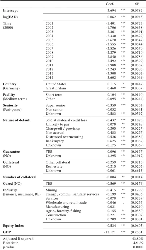
In the multiple regression model, the TTR serves as the dependent variable8while the quantities of Table 1.1 are used as regressors. Standard errors are clustered by year. Table 1.3 and 1.5 contain the results of the regression models for the overall data set and on country level. Inde-pendent variables are illustrated in the first column and according types (in case of categorical variables) are given in the second column.9 In a first step, general drivers of the TTR are derived. In the second part of this section, we focus on country specific differences.
1.3.1 General drivers of the TTR
Starting with the EAD, we find a significantly positive impact on the TTR in the overall data set. This implies that loans of larger size demand on average a longer TTR. The impact could be based on a higher level of complexity and administrative effort accompanied with the resolution of larger loans. In the model, the natural logarithm of the EAD is implemented. Hence, the relationship between the TTR and the loan size is characterized by a non-linear component. 8 Despite the non-negative restriction of the TTR, we apply the level specification of the linear regression due
to its higher explanatory power with respect to the adjusted R-squared compared to the log transformation. Appendix 1.A shows that our general results remain stable when regressing on log transformed TTR.
9 Noteworthy, not all categories are integrated in the subset models since some types are nonexistent in these
Table 1.3:Regression results of the TTR for the overall data set Coef. SE Intercept 3.694 *** (0.0782) log(EAD) 0.062 *** (0.0045) Time 2001 -1.401 *** (0.0723) (2000) 2002 -1.706 *** (0.0638) 2003 -2.361 *** (0.0591) 2004 -2.330 *** (0.0622) 2005 -2.670 *** (0.0547) 2006 -2.555 *** (0.0544) 2007 -2.526 *** (0.0570) 2008 -2.279 *** (0.0710) 2009 -2.840 *** (0.0786) 2010 -2.492 *** (0.0599) 2011 -2.988 *** (0.0587) 2012 -3.243 *** (0.0585) 2013 -3.300 *** (0.0604) 2014 -3.602 *** (0.1069)
Country United States 0.115 * (0.0447)
(Germany) Great Britain 0.460 *** (0.0337)
Facility Short term -0.104 *** (0.0190)
(Medium term) Other -0.095 *** (0.0244)
Seniority Super senior -0.359 *** (0.0254)
(Pari-passu) Non senior -0.032 (0.0641)
Unknown -0.583 *** (0.0592)
Nature of default Sold at material credit loss -0.432 *** (0.1023)
Unlikely to pay 0.078 ** (0.0248) Charge-off/ provision 0.205 *** (0.0227) Non accrual 0.483 *** (0.0277) Distressed restructuring 0.526 *** (0.0384) Bankruptcy 0.625 *** (0.0352) Unknown -0.175 *** (0.0369) Guarantee YES 0.096 *** (0.0177) (NO) Unknown -1.295 *** (0.3912)
Collateral Other collateral -0.259 *** (0.0215)
(NO) Real estate -0.215 *** (0.0205)
Unknown -0.061 (0.6613)
Number of collateral -0.004 ** (0.0014)
Cured(NO) YES -0.569 *** (0.0176)
Industry Mining -0.415 ** (0.1299)
(Finance, insurance, RE) Transp., commu., sanitary services -0.199 *** (0.0436)
Services -0.078 ** (0.0239)
Wholesale and retail trade -0.046 . (0.0255)
Manufacturing 0.021 (0.0290)
Agric., forestry, fishing 0.155 ** (0.0580) Construction 0.221 *** (0.0307) Unknown 0.209 *** (0.0381) Equity Index -0.534 *** (0.0605) GDP -12.171 *** (0.7551) Adjusted R-squared 43.80% F-statistic 421.92 p-value 0.0000
Notes: Results of the multiple linear regression regarding the overall data set. Significance codes: *** 0.001, ** 0.01, * 0.05,·0.1. Standard errors (SE) are clustered by year.
We include dummies for the default year of the loan contract to address two issues. Firstly, they control for time varying effects on the TTR, such as level shifts even if they are of non-linear nature. Additional impacts due to the macroeconomic environment that fail to be integrated trough variables might be indirectly taken into account as adverse conditions could have a worse impact than actually indicated by the GDP or equity indices. Secondly, time dummies might absorb effects of a potential resolution bias.10In the overall data set, the coefficients of these dummies have significantly negative impacts implying that the TTR decreases compared to the base year 2000. With exception of the years 2004, 2010, and the time period from 2006 to 2008, they are monotonously decreasing. This indicates a shorter resolution of distressed loans in recent years. The years 2004, 2010, and the period from 2006 to 2008 are marked by economic turmoil.11The breaks of the monotony in these years seems to refer to a rather longer TTR in a hard economic environment.
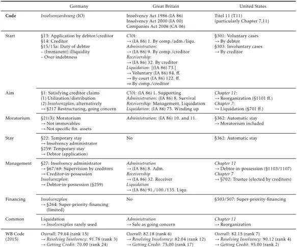
To analyze country specific differences, we primarily focus on the country dummies in this section.12 In Section 1.2, we determined the on average shortest TTR in the United States (1.26 years) and a rather longer one in Germany (1.52 years) and Great Britain (1.54 years). After controlling for other variables, a different picture appears. With Germany being the reference category, the coefficients of the country dummies show a significantly positive sign. This suggests that the resolution time isceteris paribus(c.p.) on average 0.1 years longer in the United States and even 0.5 years longer in Great Britain compared to Germany. This results seems to relate to the efficiency of default resolution. Again, we refer to theDoing Business series of the World Bank (see World Bank, 2015a,b,c,d). Under the sectionResolving Insolvency, the efficiency of the regulatory framework regarding the resolution of an insolvent company is evaluated. Thereby, a survey process is adopted and verified through a study of insolvency laws and regulations. Several assumptions about the insolvent company, the case, and the parties are made.13 The score is inspired by the methodology in Djankov et al. (2008) and expressed as a distance to frontier with 100 representing optimality. It is calculated contingent on two equally weighted indicators, namely,Recovery RateandStrength of Insolvency Framework Index. Thereby, the first is computed based on the reported time, costs, and outcome of the insolvency proceeding. The latter arises from several legal and regulatory conditions. According to this score, Germany reaches the third place with a score of 91.78 closely followed by the United 10The resolution bias belongs to the topic of sample selection. Excluding loans which are not completely resolved
leads to averagely shorter TTR in the recent years and might cause distorted parameter estimates (see Section 1.4).
11The time period from 2006 to 2008 represents the global financial crisis. The year 2010 is shaped by the European
debt crisis.
12A deeper insight into the deviations among the countries is presented in Section 1.3.2.
States with a score of 90.12 (fourth place). Amongst the considered countries, Great Britain is at the bottom of the range (82.04, 12th place). Thus, our results are confirmed by the World Bank score even though it is a purely judgmental survey process.
The variable facility distinguishes betweenmedium termandshort term. Whereas,medium term is defined as the reference. Theshort termcategory shows a significantly negative coefficient indicating that these loans tend to exhibit a shorter TTR compared to the reference category. This is noteworthy since we controlled for other more intuitive determinants, e.g., size, guarantees, and collateral. Possible explanations might be found in higher efforts with respect to resolving a medium termfacility.
Regarding seniority, loans are divided in the categoriessuper senior,pari-passu, andnon senior. The categorynon seniorcombines the original categoriessubordinated/juniorandequity. This pooling seems necessary owing to the quantity of both categories. The categorypari-passuserves as the reference. The coefficients ofsuper seniorandnon seniorshow negative signs. However, significance can only be observed for the first one. This indicates that loans of the category non seniordo not show a significantly different TTR compared topari-passu. The seniority type super senior, however, exhibits a shorter TTR which can be ascribed to the general nature of this category. Among the differences in the insolvency procedures of Germany, Great Britain, and the United States, a committee of creditors is involved leastwise at one point of the process.14 Being the one and only preferred claimant might grant this creditor comprehensive rights in the considered committees which can result in a shorter TTR.
As stated in Section 1.2, our analysis is based on defaulted loan contracts according to the definition set by the Basel Committee on Banking Supervision (2006). Thereby, default occurs either if the debtor is ”unlikely to pay” or ”past due more than 90 days on any material credit obligation” (§452). Thus, the main categories90 days past dueandunlikely to payare integrated in the model. In the data base, five additional categories are indicated. These are graded as subcategories of the more general oneunlikely to pay. Thereby, leeway in recording specific loan contracts is granted since it can be chosen between the general nature of defaultunlikely to payor a more specific one (bankruptcy,charge-off/provision,sold at material credit loss,distressed restructuring,non accrual). We do not to summarize these categories since they might supply additional information in the model context. The default definition 90 days past dueserves as the reference category. All dummy variables show statistically significant coefficients. The signs are mostly positive, except the one ofsold at material credit loss. This corresponds with 14SeeInsolvenzordung(§67, 69), Insolvency Act 1986 (4., 24., 98.), and Chapter 11 (§1102, 1126).
economic intuition: Selling an engagement should be linked to a rather short resolution process as the effort of either restructuring or liquidation is avoided. Loans defaulted due tobankruptcy tend to have on average the longest TTR since the involvement of public institutions – like courts – enhances the resolution process. Similar assumptions could be made regarding the categorydistressed restructuring.
The guarantee indicator shows a significantly positive sign indicating that loans provided with guarantees take on average longer to resolve. The fact that additional claims have to be established against the guarantor could lead to the observed increase. According Table 1.1, guarantees are more common in the United States (44.14%) than in Great Britain (34.05%) or Germany (24.44%).
However, collateralization seems to be a more common protection mechanism compared to guarantees. While 68.85% of all loan contracts exhibit segregation rights against one or more specific assets, only 31.88% include additional protection in form of guarantees. The collateral indicator is divided in the categories NO,other collateral, andreal estate. Since the loans are partly secured by several assets, real estateis indicated if at least one of them is a property. Therefore,other collateralclarifies that there is no real estate among the related securities. The coefficients of the categoriesother collateralandreal estateshow a significantly negative sign implying that collateral in general yields to a shorter TTR. A reason for this could lie in the simplicity and velocity of selling an identified asset compared to winding up the company or engaging a restructuring procedure. The coefficient of the categoryother collateralis slightly lower than the one ofreal estate. Accordingly, other assets seem to have a more decreasing effect on the TTR. This is in line with the economic intuition sinceother collateralcontains not only common assets, e.g., machinery, but also cash and general accounts which are easier and faster to liquidate compared toreal estate. Investigating the impact for the number of collateral per loan, we find a significantly negative impact.
Thecuredindicator provides information regarding the outcome of the resolution process. If a loan contract is classified as cured, it returned to performing, i.e., the obligor is back to a sound rating. This implies that outstanding claims – in the form of principal and interest obligations – will be fulfilled nearby. In the model,NOserves as the reference category. The curedindicator shows a significantly negative sign indicating a shorter TTR of loan contracts which returned to performing. These findings are in line with the results found by G ¨urtler and Hibbeln (2013), whose analysis is based on a data set provided by a German bank. They detect loans returning back to performance exhibit a shorter TTR.