Identifying key variables and interactions in statistical models
of building energy consumption using regularization
David Hsu
*210 S 34th Street, Philadelphia, PA 19104, USA
a r t i c l e i n f o
Article history:Received 2 September 2014 Received in revised form 9 January 2015 Accepted 4 February 2015 Available online 6 March 2015 Keywords: Energy consumption Buildings Variable selection Statistical models
a b s t r a c t
Statistical models can only be as good as the data put into them. Data about energy consumption continues to grow, particularly its non-technical aspects, but these variables are often interpreted differently among disciplines, datasets, and contexts. Selecting key variables and interactions is therefore an important step in achieving more accurate predictions, better interpretation, and identification of key subgroups for further analysis.
This paper therefore makes two main contributions to the modeling and analysis of energy con-sumption of buildings. First, it introduces regularization, also known as penalized regression, for prin-cipled selection of variables and interactions. Second, this approach is demonstrated by application to a comprehensive dataset of energy consumption for commercial office and multifamily buildings in New York City. Using cross-validation, this paperfinds that a newly-developed method, hierarchical group-lasso regularization, significantly outperforms ridge, lasso, elastic net and ordinary least squares ap-proaches in terms of prediction accuracy; develops a parsimonious model for large New York City buildings; and identifies several interactions between technical and non-technical parameters for further analysis, policy development and targeting. This method is generalizable to other local contexts, and is likely to be useful for the modeling of other sectors of energy consumption as well.
©2015 The Author. Published by Elsevier Ltd. This is an open access article under the CC BY license (http://creativecommons.org/licenses/by/4.0/).
1. Introduction
Statistical models enable empirically-observed measurements, that is, data from the real world, to be interpreted in terms of theory. In the phenomena of energy consumption, while physical laws and theories may governhowpeople can consume energy, there of course also important economic, social, behavioral, and geographic dimensions that explain other aspects of how people consume energy, most importantlywhy, but alsowho,where, and how much. Data for non-technical aspects of energy consumption have become increasingly available from new sources, and co-incides with growing recognition of the importance of this data for modeling, analysis, and understanding [1,2]. However, many of these non-technical aspects are often interpreted differently among various disciplines, datasets, and geographic contexts. This paper therefore addresses the critical issue of variable selection in sta-tistical models of energy consumption, because as this paper will show, this issue affects many of the goals of statistical modeling,
including accurate predictions, the interpretation of effects, and identification of key subgroups for further physics-based modeling and analysis.
This paper uses the sector of building energy consumption as a primary example because it is important in its own right, but also because it represents broadly how statistical models are used in modeling and analysis. Approximately 40% of all primary energy worldwide is consumed in and by buildings[3]. Increasing the ef-ficiency of buildings has been consistently identified over the past 40 years as a key strategy towards combating climate change and reducing energy consumption[4]. This has led to great interest in policies intended to reduce energy consumption in building stock, such as energy codes, labeling schemes, and technical standards for selected building systems. For existing building stock, proposed physical measures include weatherization, retrofit, and retro-commissioning, as well as management measures such as opera-tional and performance standards and behavioral feedback.
However, it can be difficult for many reasons to use the results of statistical models of building energy consumption to inform further modeling, analysis, and particularly, policy development such as regulations and standards; these reasons are most likely shared in other areas of energy analysis. First, rich variation in the built *Tel.:þ1 215 746 8543; fax:þ1 215 898 5731.
E-mail address:[email protected].
Contents lists available atScienceDirect
Energy
j o u r n a l h o me p a g e : w w w . e l s e v i e r . c o m/ l o ca t e / e n e r g y
http://dx.doi.org/10.1016/j.energy.2015.02.008
environment makes it possible to identify an almost unlimited number of possible factors and interactions that determine how buildings are built, occupied, modified, and consequently use en-ergy. Second, overly narrow disciplinary focus on particular pre-dictors may omit important interactions within the broader population of interest. Third, it is often difficult to generalize results from one context to another, sometimes because of lack of matching data, but also because fundamental interactions may differ by geographic context, with different people, policies and regulations, and infrastructure systems. Fourth, because it is expensive to gather comprehensive data, whether on buildings or in other sectors, results are often based on small underlying data-sets, which leads to two additional and interrelated problems. Fifth, statistical models often do not predict well out-of-sample, partic-ularly when based on small samples. Sixth, in high-dimensional problems that have more p (predictors) than n (observations), models can be easily overfit or‘saturated’, leading to wrong in-ferences and/or poor predictions.
Variable selection is therefore a critical but largely unaddressed issue in the energy consumption literature. The following review of related work will describe the key strands of the academic litera-ture, including: the interaction between physics-based and statis-tical models; the wide range of prospective new data sources; and the opportunities of “big” data. The review will also show that while there is an active andflourishing literature on variable se-lection in statistics, these methods have been little used in the modeling and analysis of energy consumption.
This paper therefore makes two main contributions, one methodological and one empirical. First, it introduces regulariza-tion to the energy consumpregulariza-tion literature, also known as penalized regression, specifically to select key variables and interactions and thereby to improve both prediction and interpretation of statistical models. The effectiveness of ridge, lasso, and elastic net methods are described for variable selection. A recently developed exten-sion, HGLR (hierarchical group-lasso regularization), is introduced because it can be used with the data structures typical of buildings and their related energy consumption, including important cate-gorical data and interaction effects. Second, this paper demon-strates this approach to variable selection by modeling a comprehensive dataset of energy consumption using a wide variety of both technical and non-technical parameters for commercial office and multifamily buildings in New York City. This is an important example that constitutes a large and diverse scale of governance and policymaking, and one that is being studied increasingly by other researchers. A dataset of whole building en-ergy consumption and many non-technical parameters for nearly one-third of all large buildings in New York City was assembled from diverse data sources, including the city's energy bench-marking laws and property tax data, as well asfinancial informa-tion from the real estate informainforma-tion providers and social and demographic information from the U.S. Census.
The next section will briefly summarize the broad literature on modeling energy consumption in buildings. The middle sections of this paper will describe the application of the lasso for model and variable selection, construction of the dataset, and discuss the re-sults. The paper concludes with a discussion of how this approach might be further applied in other areas of energy modeling and analysis, energy efficiency, and policy design.
2. Related work
2.1. Relationship of physics-based and statistical models
The literature on how to model and measure the energy con-sumption of buildings is very large. This section will therefore focus
on how empirical data and theory interact in the modeling of building energy consumption.
Models of building energy consumption are often divided into physics-based simulation and purely statistical approaches. The particulars of their application may depend on the scale at which they are used, but physics-based simulation models are typically based on theories of thermal diffusion and heat transfer, while sta-tistical models simply assume a mathematical relationship between observed energy consumption and building characteristics. This distinction is similar to the concept in systems engineering of white box and black box models, which either proceed fromfirst principles or no prior model, or theory-driven versus data-driven approaches. Physics-based simulation models are the dominant approach in the building industry. Recent surveys of building energy simulation programs discuss the inputs required for modeling, including but not limited to, their general modeling approaches; building enve-lope and geometries; daylighting and solar exposure; multi-zone airflow; renewable energy systems; electrical systems and equip-ment; HVAC (Heating, ventilation, air-conditioning and cooling) systems and equipment; occupancy patterns; and so on[5e7]. This level of detail is attractive because it enables modeling of the impact of changing particular technologies or construction methods. Still, physics-based simulation models require many data inputs about the technologies, processes, and behaviors that result in energy consumption in buildings, and then apply assumptions about how these interact. In order to model the aggregate energy consumption of many buildings, assumptions often must be made about the distribution of particular building features in the popu-lation, such as ages, sizes, and construction[8].
In contrast, statistical models are usually thought of as purely mathematical relationships between the variables. Regression analysis specifies how various covariates are combined with random variables in order to predict the energy consumption for the average building. Regression analysis can be performed on in-dividual buildings, given enough repeated measurements; or on entire populations or sectors of interest, given aggregate statistics or assumptions about the distribution of archetype buildings[9].
In practice, however, this distinction is not so readily discerned, because both model types have inherent limitations, and because these two types of models are often used to inform one another. On one hand, while physics-based models may be useful as a heuristic measure or tool during the design or construction phase, they often do not describe accurately the energy consumption of buildings when they are actually occupied, operated, managed, and main-tained. There is a significant body of evidence that building energy simulation models deviate significantly from observed energy performance, which has stimulated thinking about how to measure the observed performance of buildings differently [10e13]. A comprehensive survey[14]classifies the factors that contribute to the commonly observed gap between predicted and observed en-ergy consumption, andfinds that they can stem from the various stages in which buildings are modeled and operated, including the processes of design, construction, handover, and actual operation. Statistical models are therefore sometimes used to evaluate the performance of energy analysis models.
On the other hand, physics-based theories and assumptions are still necessary in statistical models to determine which variables are considered to be important, and how they should be defined and combined, and in what functional model specification, with linear or nonlinear relationships, or distribution of random errors, and so on. Many inputs into physics-based models are based on studies of building or material parameters, and a great deal of recent work has focused on how to calibrate model structure ac-cording to observed consumption, decompose larger models into smaller ones, and incorporate parameter uncertainty[15e22]. In
summary, physics-based and statistical models can be used to inform one another in the modeling and analysis of building energy consumption.
2.2. Multiple disciplines and variables
However, a major complication to both the physics-based and statistical approaches, and the general study of building energy consumption, is the sheer range of variables that prospectively affect building energy consumption. Physics-based models may require hundreds of engineering or physical measurements. Furthermore, interest in non-technical factors has grown, such as political, social, legal, psychological, behavioral, organizational, and demographic factors.
There is a rapidly growing literature detailing a wide range of factors that affect the observed energy consumption of actual buildings, such as different facility types, ownership patterns, occupant behaviors, and so on. Examples include occupancy pat-terns [23]; occupant behavior and comfort [24,25]; building maintenance practices [26]; the use of building intelligence and controls[27]; appliance or plug loads in buildings; or low-income residents[28]. Further work is needed in order to integrate the existing literature on technical factors in energy consumption with the wide range of possible non-technical factors.
2.3. “Big”data approaches
Increasing amounts of data, or so-called “big data”, has considerable potential to address these gaps. Disclosure laws are increasingly making large amounts of data available about energy consumption in buildings, but there are still a number of concep-tual and quality issues associated with self-reported data [29]. Administrative databases, such as property tax, construction permitting, and building inspection databases maintained by mu-nicipalities, may contain important information about building physical characteristics, as well as zoning, lot, andfinancial infor-mation. Commercial property brokers may also have a great deal of information about the financial and quality characteristics of buildings. Other prospective sources of information are sub-metered or sensor information at smaller scales within buildings; schedules and operations maintained by building staff; databases about energy systems and conservation measures maintained by utilities; operational databases maintained by building contractors or service staff. Most importantly, much of this data can and is being joined or‘federated’together.
Some work has already been done with relatively large new datasets. A study on a subset of comparable buildings in Stockholm used principal components analysis and partial least squares in order to identify key determinants of consumption for district heating consumption, building electricity use, cold water con-sumption, and total heat loss [30], and another used machine learning methods in order to identify the appropriate level of spatial and temporal granularity to forecast energy consumption in multifamily residential buildings[31]. As the amount of data con-tinues to increase in new studies, such as in Refs. [32], variable selection methods are necessary to identify key determinants of building energy consumption.
2.4. Variable selection as a key analysis issue
While OLS (ordinary least squares) regression remains a popular workhorse method because it is computationally straightforward and results in unbiased coefficients, depending on the conditioning and structure of the data itself, OLS can still result in biased co-efficients that are inflated in magnitude, have the wrong signs, or
which radically change depending on the model and variables that are selected[33].
For structured data withnunits or observations, andpfeatures, as p grows, the number of possible models quickly becomes intractable, with 2ppossible models with subsets of thepfeatures. Merelyp¼20 gives over a million possible subsets of features and therefore potential models to evaluate. Furthermore, if pairwise interactions are further included between predictors, then the additional number of possible interactions is described by the binomial coefficient
p 2
: merely p¼200 gives almost 20,000 additional possible models with interactions. Regression in high-dimensions when p>n introduces other structural problems. Since any vector of outcomes can be formed as a linear combi-nation of a sufficiently large number of predictor vectors, including too many predictors can lead to overfitting. Including too many predictors and unbiased coefficients leads to higher variance in out-of-sample mean squared error, and therefore less accurate predictions, in the well-known tradeoff between bias and variance error. Finally, models containing many features are difficult to interpret; parsimony is therefore an important value to strive for.
As a result, there is a large and active literature on variable se-lection in statistics. The lasso introduced by Tibshirani [34] is particularly useful for model and variable selection, particularly in large datasets wherenandpare large; in high-dimensional situ-ations, wherep>n[33]; and even in the presence of noisy variables [35e37].
The energy consumption literature seems not to have used regularization methods very much at all. Searching for the exact phrases “penalized regression” or “regularization” in Google Scholar yields only one paper in the core energy journals (Energy, Energy Policy, and Applied Energy). Searching for the names of specific methods such as“lasso”and“ridge”yields only a few more papers (10e20), mostly in economic models of energy use.
A few other studies have used different methods to identify key variables for energy consumption and modeling. Zhao and Magoules[38]has the most comprehensive literature review but they toofind little previous work concerned with feature selection, and their subsequent approach is to apply support vector regres-sion to select subsets of features to predict energy consumption. Other methods have been used to select or filter variables in particular situations, including principal components analysis of energy use[39], and neural networks and data mining methods to detect outliers[40]and faults[41].
3. Methodology 3.1. Regularization
This section will describe a general approach to dealing with data assembled from multiple domains and sources. This section shows how penalties can be added to the regression process, in order to aid in stable and efficient estimation, and to minimize or eliminate smaller magnitude coefficients in order to aid inter-pretation. The general linear regression problem is, in matrix notation:
Y¼Xbþε (1)
whereYis an1 vector;Xis thenpmatrix of predictors;
b
is thep-length vector of coefficients to be estimated; andεis normally distributed with mean zero and a constant (and unknown) variance of s2. Ordinary least squares (OLS) regression estimatesb
by minimizing the RSS (residual sum-of-squares) with respect tob
:argmin
b RSSðbÞ ¼
YXb2 (2)
Penalized regression methods broadly restate the problem of estimating coefficients as constrained optimization problems by adding penalties to the regression coefficients to achieve particular goals. Hoerl and Kennard [42] developed ridge regression to compare directly the importance of individual factors. Tibshirani [34]introduced the lasso method in order to add a differently-structured penalty that allows both continuous shrinkage and variable selection. Zou and Hastie[43]subsequently introduced the elastic net, which combines the ridge and lasso penalties. All of these approaches can be generally stated using the following like-lihood functionL, which is a function of parametersl1,l2, and the vector
b
:Lðl1;l2;bÞ ¼YXb2þl2b2þl1b
1 (3)
where the penalty terms are adjusted byl1andl2, respectively: b2¼X p j¼1 b2 j; and b1¼ Xp j¼1 bj (4)
Also, because the likelihood function and penalties depend on the magnitude of the coefficients, the columns of the responseY
and the predictor matrixXare centered and standardized to have mean zero and a standard deviation of 1. Lettinga¼l2=ðl1þl2Þ, the estimator for the coefficient vector
b
can then be stated as the following optimization problem:argmin b YXb2; subject toð1aÞb 1þab 2 tfor somet: (5) where the “budget” constraint on the coefficients is
ð1aÞb1þab2, also known as the elastic net penalty. Ifa¼0, this becomes the lasso penalty; ifa¼1, this becomes the ridge penalty. Closed form solutions can be obtained for OLS and ridge regression, but for the lasso and elastic net, estimation of the co-efficient vector
b
does not have a closed form solution because of the nonlinearities introduced by the absolute value sign, and must be estimated using optimization methods. Hastie et al. [33, pages 91] provide a thorough introduction to regularization, particularly for variable selection. The following subsections will describe properties of particular extensions of the lasso that can be used in order to address common issues in high-dimensional, multi-domain building energy data, and the software packages used to compute the different optimization problems.3.2. Other key issues
Three structural issues commonly arise in variable selection: multicollinearity, categorical predictors, and interactions. Each of these problems will be discussed in turn, and how these issues can be addressed using extensions of the lasso method.
First, multicollinearity is quite common in multi-domain data-sets, in which each dataset may contain predictors for a similar aspect of the observations, or in which particular predictors are simply high-correlated naturally. The elastic net penalty, a combi-nation of the ridge and lasso penalties, most effectively deals with multicollinearity, a common problem, particularly in high-dimensional regression wherep[n[43].
Second, categorical variables are quite common in data on building energy consumption, such as what type of heating system a building might have; the type of property use, or the type of ownership orfinancing structure. This is addressed using the group lasso, an extension of the lasso, in which entire groups of co-efficients enter the minimization criteria together or in ensembles, allowing categorical data or factors to be included or discarded from the optimization problem[44e46].
Third, andfinally, with high-dimensional, multi-domain data-sets, it is possible and interesting for there to exist a large number of unknown interactions, particularly between unrelated datasets. For example, it is plausible that predictors describing energy sys-tems and socio-demographic characteristics may interact in pre-dicting energy consumption behavior, or that predictors describing the use and maintenance of a space may affect its related energy consumption. As noted above, the number of possible pairwise interactions betweenppredictors is
p 2
.
One of the most attractive features of regularization methods such as the lasso is that it can be modified to take into account all of these issues. Yuan and Lin[44]introduced a group lasso formulation that allows variables to be grouped, therefore allowing predictors to be either categorical or continuous, and Bien et al.[47]introduce con-straints that preserve strong or weak hierarchy between interactions. Lim and Hastie[48]combine these improvements into hierarchical group lasso regularization (HGLR), which allow both continuous and categorical variables to be included, as well as all of the pairwise in-teractions between them, to be included as overlapping group lasso problems, with an enforced hierarchy in the interactions only be-tween the categorical levels. Non-zero coefficients for these cate-gorical variables are interpreted as differences from the estimated intercept, rather than from any reference category.
For HGLR, the model for the vector of quantitative responseYis:
Y¼mþX p i¼1 Xiqiþ X i<j Xi:jqi:jþε (6)
with intercept
m
, theith column of predictor matrix Xiwithp fea-tures as either categorical and continuous variables, and in-teractions between variables denoted by Xi:j. The loss function for the squared error loss is given by:LY;Xi:ip;Xi:j;m;q¼1 2 Ym,1þX p i¼1 XiqiþX i<j Xi:jqi:j2 2 (7) The optimization problem for the group-lasso obtains estimates as the solution to:
argmin m;b 1 2 Ym,1X j¼1 p Xjbj2 2 þlXp j¼1 gjbj 2 (8)
where
l
and thegjare used to penalize all of the coefficients and separate groups differently. Different groups of main effects and in-teractions can be added to the group-lasso problem to obtain the hi-erarchical interaction model. Proofs of how this condition enforces hierarchy and algorithmic details are presented in Lim and Hastie[48].3.3. Model selection&validation
This paper does not calculate the significance of the variables for several reasons. The chi-squared test is typically used to evaluate the addition of variables in two nested models. First, with datasets that are large in the number of observationsnand the number of predictorsp, it is relatively easy to get statistical but not practical
significance. Second, since each model has a varying number of parameters, each model would require adjustment of the numbers of degrees of freedom in each chi-squared test. Third, lasso-type models require test statistics that reflect the significance of the predictors entering the model sequentially or adaptively, in contrast to typical OLS approaches, which evaluate all of the pre-dictors simultaneously and which can lead to overfitting[49].
Instead, cross validation is used to obtain the most flexible model with the least amount of prediction error. The MSE (mean squared error) can be decomposed mathematically into a bias and variance component: Ey0bfðx0Þ 2 ¼Varbfðx0Þ þhBiasbfðx0Þ i2 þVarðεÞ (9)
whereEis the expectation, y0 is the observed response, and bfðx0Þis the prediction atx0. The lowest MSE will be the result of a
low bias and low variance component. This is obtained by first sampling approximately 90% of the observations (the training dataset),fitting a model, and then using thefitted model to predict the remaining 10% of the dataset (a test dataset). Each time this is done is called a“fold”. This is then performed ten times in order to calculate the most effective tuning value in terms of the MSE and its associated standard deviation. The most effective tuning value is typically taken at the lowest mean squared error, or within one standard deviation of the minimum, because of the inherent error in the MSE prediction itself over multiple folds.
One of the reviewers helpfully suggested that the stability of the variable selection process could be tested using bootstrapping methods. While application of these methods could not befit into the scope of this paper, the stability of feature selection has already been investigated using bootstrapping methods in a number of papers. Yuan and Lin[44]use bootstrapping methods tofind that the lasso and related methods with grouped variables are much more stable than traditional backwards-stepwise selection methods. Studies of the stability of lasso-based feature selection using bootstrapping are discussed in He and Yu[50], Meinshausen and Bühlmann[51]and Tibshirani[52].
3.4. Software
The lasso, elastic net, and ridge can all be computed using the glmnet package for the statistical software R. The HGLR method is computed using the glinternet package. All are available from www.cran.us.r-project.org[53e55].
4. Data
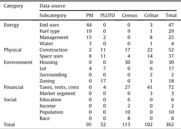
A comprehensive dataset from multiple domains was assembled in order to apply and evaluate different modeling methods for building energy consumption. Datasets for large buildings in New York City in both multifamily and commercial office categories were assembled, because large buildings represent 48% of all primary en-ergy use in New York City (compared to 17% transportation and 35% from small buildings), and multifamily and office buildings represent 87% of all grossfloor area of all large buildings[56]. The datasets were assembled from multiple data sources, including the U.S. Environ-mental Protection Agency's Portfolio Manager, the City of New York's PLUTO (primary land use tax lot output) database, real estate and financial information from the CoStar Group, and tract level infor-mation from the U.S. Census, including inforinfor-mation from the 2010 decadal Census, the 2011 American Housing Survey, and the 2013 ACS (American Community Survey).Table 1shows the general categories of information contained in each dataset, which frequently overlap in particular categories. The following section will describe how the data was cleaned, assembled, and treated for analysis.
The outcome variable to be modeled is the logarithm of site (metered, orfinal, as defined by EN-ISO) EUI (energy use intensity) of buildings, which is measured by energy use per unit area and is an intensive quantity, rather than the total energy use, an extensive quantity. The choice to model EUI was retained so results can be compared to other existing approaches, and the logarithm was used to correct for the extreme lefthand skew of the distribution of EUIs (i.e., there are many more low-intensity buildings than high). Site energy is used because all of the buildings are in the same region and to avoid using regional conversion factors to source (primary) energy.
Data about energy performance and specific end-use charac-teristics was obtained through the City of New York's annual benchmarking ordinance for commercial and multifamily build-ings, Local Law 84. The City of New York collects whole-property energy benchmarking data for commercial and multifamily prop-erties over 4645 square meters (50,000 square feet) using the U.S. Environmental Protection Agency's Portfolio Manager interface, including annualized energy use by fuel type, the distribution of space uses within the buildings, and selected measurements of end-uses for certain facility types. Energy information for parcels was then joined to key property and construction characteristics contained in City of New York's PLUTO database using unique parcel identification numbers. Furthermore, each of these parcels can be located within a unique census tract using the City's parcel shapefiles and the U.S. Census TIGER shapefiles. U.S. Census data was therefore downloaded for the 2010 Census, 2011 American Housing Survey, and the 2013 American Community Survey from the American FactFinder website. The census information was then spatially joined to each parcel using ArcGIS. CoStarfinancial infor-mation for the individual buildings was downloaded in February 2014. This information is gathered on a continuing basis from property sales and leasing brokers. After joining the parcels, this resulted in 5638 uniquely identified buildings, with complete en-ergy, tax, census, andfinancial information.
The dataset was then limited to multifamily housing and office buildings as classified in the Portfolio Manager database, resulting in 4072 multifamily and 937 office buildings. This classification is defined as when more than 50% of the gross area is used for that space use. This was further limited to buildings that constitute more then 75% of multifamily housing and office, respectively, since this eliminated only 4% of each category, and in order to get only the buildings typical of each category. This resulted in 4815 Table 1
Table Showing Number and Type of Variables from Each Dataset. Some of these variables are later eliminated in the cleaning process.
Category Data source
Subcategory PM PLUTO Census CoStar Total
Energy End uses 44 0 0 3 47
Fuel type 19 0 9 1 29 Management 15 2 0 8 25 Water 3 0 0 1 4 Physical Construction 2 11 17 22 52 Space uses 8 11 4 14 37 Environment Housing 0 0 30 0 30 Lot 4 7 0 6 17 Surrounding 0 0 0 2 2 Zoning 0 17 0 1 18
Financial Taxes, rents, costs 0 4 27 41 72
Market segment 0 0 0 3 3 Social Education 0 0 6 0 6 Income 0 0 2 0 2 Population 0 0 10 0 10 Race 0 0 8 0 8 Total 95 52 113 102 362
buildings, comprised of 3941 multifamily housing buildings and 874 office buildings.
Data for individual buildings then required further extensive cleaning and treatment for analysis, particularly between contin-uous and categorical variables. Buildings with an EUI of less than 0.15 and greater than 3.15 kWh per square meter per year were eliminated as data that was unlikely to be correct due to engi-neering judgement. For continuous variables that constituted a component of a total, such as one fuel type among many, or a portion of the overall population, percentages were calculated. Skew and kurtosis measurements were used to determine if loga-rithmic transforms were necessary in order to obtain systematically distributed independent variables, and therefore are expected to yield residuals that follow the normal distribution. Columns for continuous variables were eliminated entirely only if they were empty: for example, very few office buildings indicated information in the multifamily housingfields, and similarly, very few multi-family buildings contain any information about data centers. In-formation about individual buildings contained in text fields in Portfolio Manager and CoStar were transformed into dummy var-iables, such as information about amenities such as dishwashers or a property manager on site.
In order to ease both interpretation and estimation time, cate-gorical variables were eliminated if they resulted in too many sparsely populated levels, since this data is relatively unimportant compared to larger segments in the broader population. Similarly, the number of levels for each categorical variable was reduced by reclassifying any levels with a small number of observations (less than 20) into an“other”category, and then removing any buildings entirely with a small number of observations (less than 10) for any given categorical variable. These cleaning steps affected less than 1% of the data. Finally, any continuous and categorical columns that were perfectly correlated (with Pearson's
r
¼1) were eliminated, since these constitute the same data. This was usually the same data from multiple data sources. In penalized regression, all nu-merical coefficients must be standardized, since they are being penalized on the same scale. Indicator or dummy variables for categorical variables were not standardized.The resulting datasets for the analysis have 3902 multifamily housing buildings and the 846 office buildings, respectively. The number of categorical, continuous, and interaction variables is detailed in Table 2. Descriptive statistics for key variables are described inTable 3.
5. Results&discussion
The lasso, elastic net, and ridge models are all applied to the same dataset, although to apply these methods, categorical vari-ables and interactions must be recoded as a column of dummy indicator variables. Every possible interaction between continuous and categorical variables was allowed. This gives many possible interactions, 7402 for multifamily housing and 2023 for office buildings, which varies between the two datasets because of the different numbers of categorical levels eliminated in the cleaning process. Both are slightly less than the theoretical maximum of
p 2
, because levels of the same categorical variable do not interact with one another. In both cases, however,p[n, making this a high-dimensional problem with potential overfitting.
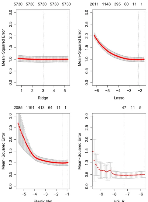
Figs. 1 and 2show the cross-validation results used to select the optimal
l
values, and therefore the optimum tuning or number of variables. Ten-fold cross validation is used to calculate the mean and standard error of the predictions. All of the models exhibit the classic U-shape of the bias-variance tradeoff. Ridge regression characteristically does not remove any variables, while the elastic net, lasso, and HGLR approaches all remove significant numbers of variables. The vertical axis shows that HGLR significantly out-performs the ridge, lasso, and elastic net approaches in terms of prediction error. Putting more structure into the optimization problem in terms of distinguishing between continuous and cate-gorical variables, and imposing hierarchical constraints on which interactions can be included, results in a 50% and 60% reduction in prediction error for multifamily and office buildings, respectively.Also,Figs. 1 and 2indicate that an incredibly small number of variables can be effective for cross-validated predictions. In com-mercial buildings,Fig. 1shows that HGLRfinds that as few as 6-10 variables can be used to obtain a MSE (mean squared error) for prediction that is within a standard deviation of the absolute minimum MSE obtained by models with 30e60 variables. For multifamily buildings, Fig. 2shows that one key variable can be used to obtain a prediction MSE that is within a standard deviation of models with 5e50 variables. This means that with proper identification of variables, future data collection requirements for similar analyses could be much less than needed at present.
The results obtained using HGLR were also compared to existing approaches. OLS could not be used because of the large number of interactions (7402 for multifamily and 2023 for office) already overfits the number of observed outcomes (3902 for multifamily and 846 for office). In order to provide a fair baseline comparison, variables identified from EPA's Energy Star technical methodology are used[57]. In order to provide a fair comparison similar to the existing Energy Star benchmarking methodology, the same vari-ables and regression models were used but new regression models Table 2
Descriptive statistics for multifamily and office data.
Number Multifamily Office
Observations (n) 3902 830
Continuous variables (pcont) 256 245
Categorical variables (pcat) 37 37
Categorical levels (m) 161 86
Pairwise interactions (Xi:j) 7402 2023
Table 3
Descriptive statistics for key continuous variables, including fuel use and types, space uses, andfinancial characteristics.
Variable Multifamily Office
Min. Mean Max. Min. Mean Max. Year built 1850 1947 2012 1600 1935 2009 Fuel use (% of Total)
Electricity 0.0 0.3 1.0 0.0 0.6 1.0 Natural gas 0.0 0.4 1.0 0.0 0.1 0.9 District steam 0.0 0.0 0.9 0.0 0.1 1.0 Fuel oil 2 0.0 0.0 1.0 0.0 0.0 0.8 Fuel oil 4 0.0 0.1 1.0 0.0 0.0 1.0 Fuel oil 56 0.0 0.2 1.0 0.0 0.1 1.0 Other 0.0 0.0 0.5 0.0 0.0 0.0
Space uses (LogSqFt)
Total 9.1 11.5 13.8 9.5 12.1 14.8
Multifamily, gross 9.1 11.5 13.8 0.0 0.0 0.0 Multifamily, taxed 0.0 11.2 13.9 0.0 0.0 0.0 Multifamily units (No.) 0.7 4.4 7.3 0.0 0.0 0.0
Office, gross 0.0 0.6 11.2 0.0 0.0 0.0
Office, taxed 0.0 1.4 12.4 9.1 11.5 13.8
Parking, gross 0.0 1.2 12.4 9.5 12.1 14.7 Financial (Log USD ($))
Operating expenses 5.7 13.1 16.1 0.7 2.8 7.6 Assessed total value 12.4 15.0 18.2 0.0 0.2 12.8
Tax per area 0.0 1.3 5.6 13.3 16.6 20.3
were applied to the office buildings specifically in the New York dataset. When the penalized regression methods are compared to existing OLS approaches inTable 4, OLS for office buildings using the variables selected in the USEPA's (U.S. Environmental Protec-tion Agency) Energy Star methodology performs on par with the lasso, ridge, and elastic net methods, all of which use different numbers of variables, but significantly underperforms the HGLR method, which predicts with 50% less relative MSE.
Ridge traces, or plots of coefficients versus the tuning parameter
l
show the relative importance of variables. Only the ridge traces for the HGLR approach for multifamily and office buildings are shown in Figs. 3 and 4, respectively. The top variables for each category are shown inTables 5 and 6. The variables selected in the two models and building types are very different.For multifamily buildings, the top main effects inTable 5are the percentage of total energy from electricity (0.58) and the per-centage of nearby buildings built in the 1970s (1.13). Several
indicators of space uses, such as the percentage of medical office cooled (0.33), the refrigeration retail density (0.48), and the log-arithm of the largest contiguous area in the building (4.05) all have strong effects on total energy consumption. This makes sense given the large number of mixed use buildings in New York, where almost all multifamily buildings contain other space uses, in particular large groundfloor retail areas that may consume unusual amounts of energy relative to multifamily buildings.
Notably for multifamily buildings, several socio-demographic characteristics are important and interact with the percentage of electricity used, including the percentage of African-American (main effect 0.17, interaction of0.63) and Asian residents (main effect of0.18, interaction of 0.53) in the census tract, and the percentage for which the rent-income ratio is high (0.72). These variables indicate strongly that a particular set of buildings, which consume a relatively high proportion of electricity and are situated within enclaves of these ethnic populations, deviate strongly from Fig. 1.Graph of prediction error by method and number of variables for office buildings. Vertical axis is the mean-squared prediction error, horizontal bottom axis is the logarithm of the tuning parameterl(different for each method), and the numbers on the horizontal top axis are the number of variables in each model. Center line of the curves represents the MSE (mean squared error) for 10-fold cross validation, while the grey shaded areas indicate the resulting standard error of the MSE. Vertical dotted lines indicate the optimum models selected by minimum cross-validated error (left vertical line) and the cross-validated error from the model with the least number of variables within 1 standard deviation of the minimum MSE (right vertical line).
the average building. Further investigation is of course necessary to understand the causal relationship between these variables, but this identifies two previously unknown groups of buildings, people, and effects that may constitute outliers above and below typical pattern of energy consumption.
For commercial office buildings, the top main effects inTable 6 are the percentages of energy used in four main categories: electricity (0.54), natural gas (0.28), district steam (3.86), and fuel oil 5 and 6 (0.98). The relatively high coefficient for steam en-ergy use also has interactions with electricity (4.35) and the log assessed tax per area (0.23). While the first effect is not sur-prising, since as the percentage of steam goes up, the percentage of electricity will probably go down, since they sum to 100; the second effect indicates that higher value buildings with steam systems use slightly less energy than similar steam-powered buildings.
The estimated interactions between key variables such as per-centage of energy from electricity and steam are illustrated in the contour plots inFig. 5. This plot shows that relatively small changes in the percentage of each building's energy from electricity and steam consumption can interact to have significant effects on en-ergy consumption: a half standard deviation change in both the percentage of energy from electricity and steam results in a swing of plus or minus two standard deviations in observed energy consumption.
Fig. 2.Graph of prediction error by method and number of variables for multifamily buildings. Visual elements and interpretation are the same as inFig. 1.
Table 4
Prediction error for EUI based on 10-fold cross validation. Prediction errors are re-ported as multiples of standard deviation of the observed outcome variable. OLS uses the variables selected by EPA in their technical methodology, but regresses them specifically to the NYC office dataset. The technical methodology for multi-family buildings has not yet been published.
Method Multifamily Office
Error SD Error SD OLS-NYC 0.99 1.63 Ridge 1.00 0.13 0.94 0.15 Lasso 0.99 0.10 0.86 0.10 Elastic net 0.99 0.12 0.84 0.09 HGLR 0.46 0.14 0.40 0.12
In addition, it is interesting that for office buildings, a large number of variables from the 2010 Census and 2011 American Housing Survey seem to play a role, in particular those describing the composition of surrounding multifamily units. This is a particular feature of surrounding areas for a subset of office buildings in New York City, and is another example of a useful result
in identifying particular subpopulations of interest in a local jurisdiction.
It is also worth noting that none of the categorical variables included in the analysis proved to be important determinants of energy consumption, relative to other more important continuous variables. This may indicate that the structure of the categorical variables either was not particularly important in determining energy consumption, or that variation that could be measured us-ing continuous variables within these groupus-ings was more impor-tant than any variation between the categorical groupings.
6. Conclusion
This paper began by arguing the importance of statistical models to understanding energy consumption in both buildings and other sectors. In order to overcome some of the endemic problems with the statistical modeling of energy consumption, this paper introduced a general method for variable selection to the energy consumption literature, in order to identify important Fig. 3.Graph of coefficient values versus tuning parameter, or“ridge traces”for
multifamily buildings. The vertical axis represents the coefficient values relative to one another as the tuning parameter is changed: each line denotes a different coefficient, with magnitudes plotted on a relative scale because all predictors are standardized. Again, the horizontal bottom axis is the logarithm of the tuning parameterl(different for each method), and the numbers on the horizontal top axis are the number of variables in each model. As the tuning parameter is changed from right to left, more variables and interactions progressively enter the model.
Fig. 4.Graph of coefficient values versus tuning parameter, or“ridge traces”for office buildings. Visual elements and interpretation are the same as inFig. 3above.
Table 5
Top Variables for Multifamily Buildings. Only the standardized variables with co-efficients greater than 0.1 shown. Asterisks denote variables aggregated by census tract from the 2010 Census and 2011 American Housing Survey.
Variable 1 Variable 2 b(std.)
Main effects Pct electricity 1 0.58
Medical off. pct cooled 1 0.33
Retail refrig density 1 0.48
Log max contig. Area 1 4.05
Pct black* 1 0.17
Pct asian* 1 0.18
Avg HH size owned* 1 0.12
Pct year built 1980s* 1 0.24
Pct year built 1970s* 1 1.13
Interactions Pct electricity Log assessed tax tot. 0.11 Pct electricity Pct black* 0.63 Pct electricity Pct asian* 0.53 Pct electricity Avg HH size owned* 0.58 Pct electricity Pct rent-income high* 0.72 Office Worker Density Retail Refrig. Density 0.19 LogOPExSqF Pct Year Built 1970s* 0.54 Asterisk indicates aggregated variables for the census tract of the building from the U.S. Census.
Table 6
Top Variables for Office Buildings. Only the standardized variables with coefficients greater than 0.1 shown. Asterisks denote variables aggregated by census tract from the 2010 Census and 2011 American Housing Survey.
Variable 1 Variable 2 b(std.)
Main effects Pct electricity 1 0.54
Pct natural gas 1 0.28
Pct district steam 1 3.86
Pct fuel oil 56 1 0.98
Log transit dist 1 0.41
Pct MF units (1)* 1 0.36
Pct MF units (3e4)* 1 73.02
Pct MF units (5e9)* 1 0.68
Pct more than 5 beds* 1 7.18
Pct HH bottled gas* 1 3.33
Pct no mortgage (10e15)* 1 0.23 Interactions Pct electricity Pct district steam 4.35 Pct electricity Pct Fuel Oil 56 1.18 Pct district steam Log tax per area 0.23 Log comm. Area Pct more THAN 5 beds* 0.57 Log Comm. Area Pct HH bottled gas* 0.27 Log Av. unit size Pct MF units (3e4)* 10.49 Log num. studios Pct MF units (1)* 0.20 Log num. studios Pct HH bottled gas* 1.70 Asterisk indicates aggregated variables for the census tract of the building from the U.S. Census.
variables and interactions, both from multiple, technical and non-technical, data sources. Datasets for nearly one-third of all large multifamily and commercial buildings in New York City were assembled from multiple data sources, and modeled using regularization methods. HGLR (hierarchical group-lasso regula-rization) significantly outperformed all other approaches, including the existing Energy Star technical methodology commonly used for benchmarking buildings in the United States. In addition, by building a model structure that accommodates the types of data structures and variables that commonly appear for buildings and their related energy consumption, HGLR clearly
outperformed all other methods in terms of prediction accuracy using 10-fold cross-validation. This also allowed identification of several novel interactions, specifically within New York City building stock.
Due to the rapid growth of benchmarking efforts as a major policy initiative, it is important to provide accurate predictions as a reference standard in order to measure the relative level of effi -ciency of existing buildings. Accurate prediction therefore should be the criteria for selection of variables for further research, and to understand which parts of the population may require further investigation.
Fig. 5.Interaction between electricity and steam use for office buildings. Relatively small changes in the percentage of each building's energy from electricity and steam con-sumption can interact to have significant effects on energy concon-sumption.
As demonstrated by the results above, certain variables can be isolated from the population of New York City buildings, in order to identify critical sub-populations of buildings that may have disproportionate impact on overall energy consumption and greenhouse gas emissions, and therefore constitute either partic-ularly promising (or lost) opportunities for energy efficiency. This approach would allow particular buildings to be targetedfirst in energy efficiency efforts such as through subsidies, incentives, regulation or penalties, either led by the city government or local utilities, in order to make the most effective intervention in building energy consumption.
One could object that thesefindings simply constitute correla-tions within the data and not causal relacorrela-tionships. This is possibly true, but this charge could be levied at any statistical model that is based on observational data and not on an explicitly causal or experimental research design. The intention of this analysis was to select variables through a principled statistical process in order to improve significantly out-of-sample predictions, as seen inFig. 4, and to identify key variables and interactions to support these predictions. This is an important step to support further analysis, either through subsequent physics-based or simulation models, or through additional data collection and gathering to improve sta-tistical analysis.
Furthermore, a general method for selecting key variables and interactions is important when considering how to generalize models from one context to another. Building energy consumption is subject to many local effects, including but not limited to, local construction practices, infrastructure networks, patterns of occu-pancy and use, zoning and other legal frameworks. Data is often limited in different jurisdictions. This paper demonstrated this approach in New York City, but this method could easily be applied to other scales. This is also likely true for statistical models in other sectors, beyond buildings.
Finally, robust variable selection opens up a number of other areas of research into the energy consumption of buildings. First, this should aid in more efficient data collection, since not all vari-ables are equally important for gathering, cleaning, and dissemi-nation. Second, since many classification approaches used for buildings such ask-means or hierarchical clustering are extremely sensitive to which and how many variables are used for, the key determinants of energy consumption should be used to classify buildings, and therefore reduce the overall building population to more manageable subcategories. Third, and similarly, since many efficiency and productivity measures suggested for benchmarking, such as the current technical methodology for Energy Star, as well as approaches such as data envelopment analysis and stochastic frontier analysis also critically depend on variable selection, then selecting key variables will also make more robust efficiency ana-lyses possible.
Acknowledgments&disclaimer
Thank you to the editors and three anonymous reviewers for their detailed and helpful comments, which considerably clarified and strengthened the paper.
Thank you to the City of New York Office of Long-Term Planning and Sustainability and CoStar for providing the data. Thank you to Albert Han, Daniel Suh, and Jeremy Strauss for their meticulous work in cleaning and assembly of data from many sources. Thank you to Hong Hu, Ting Meng, and Trevor Hastie for their comments and feedback. Any remaining errors in this article are solely the work of the author.
This material is based upon work supported by the Consortium for Building Energy Innovation, an energy innovation hub sponsored by the U.S. Department of Energy under Award Number DE-EE0004261.
References
[1] Schweber L, Leiringer R. Beyond the technical: a snapshot of energy and buildings research. Build Res Inform 2012;40:481e92.
[2] Sovacool BK. What are we doing here? analyzingfifteen years of energy scholarship and proposing a social science research agenda. Energy Res Soc Sci 2014;1:1e29.
[3] Perez-Lombard L, Ortiz J, Pout C. A review on buildings energy consumption information. Energy Build 2008;40:394e8.
[4] Pacala S, Socolow R. Stabilization wedges: solving the climate problem for the next 50 years with current technologies. Science 2004;305:968.
[5] Foucquier A, Robert S, Suard F, Stephan L, Jay A. State of the art in building modelling and energy performances prediction: a review. Renew Sustain Energy Rev 2013;23:272e88.
[6] Zhao HX, Magoules F. A review on the prediction of building energy con-sumption. Renew Sustain Energy Rev 2012;16:3586e92.
[7] Crawley DB, Hand JW, Kummert M, Griffith BT. Contrasting the capabilities of building energy performance simulation programs. Build Environ 2008;43: 661e73.
[8] Kavgic M, Mavrogianni A, Mumovic D, Summerfield A, Stevanovic Z, Djurovic-Petrovic M. A review of bottom-up building stock models for energy con-sumption in the residential sector. Build Environ 2010;45:1683e97. [9] Swan LG, Ugursal VI. Modeling of end-use energy consumption in the
resi-dential sector: a review of modeling techniques. Renew Sustain Energy Rev 2009;13:1819e35.
[10] Norford L, Socolow R, Hsieh E, Spadaro G. Two-to-one discrepancy between measured and predicted performance of a‘low-energy’office building: in-sights from a reconciliation based on the DOE-2 model. Energy Build 1994;21: 121e31.
[11] Chung W. Review of building energy-use performance benchmarking meth-odologies. Appl Energy 2011;88:1470e9.
[12] Frankel M, Heater M, Heller J. Sensitivity analysis: relative impact of design, commissioning, maintenance and operational variables on the energy. In: Conference proceedings of the 2012 ACEEE summer study on eneregy effi-ciency in buildings, Asilomar, CA; 2012.. In: http://www.aceee.org/files/ proceedings/2012/start.htm.
[13] Pang X, Wetter M, Bhattacharya P, Haves P. A framework for simulation-based real-time whole building performance assessment. Build Environ 2012;54: 100e8.
[14] de Wilde P. The gap between predicted and measured energy performance of buildings: a framework for investigation. Automation Constr 2014;41: 40e9.
[15] Reddy TA. Literature review on calibration of building energy simulation programs: uses, problems, procedures, uncertainty, and tools. ASHRAE Trans 2006;112:226e40.
[16] Raftery P, Keane M, Costa A. Calibrating whole building energy models: detailed case study using hourly measured data. Energy Build 2011;43:3666e79. [17] Rysanek AM, Choudhary R. A decoupled whole-building simulation engine for
rapid exhaustive search of low-carbon and low-energy building refurbish-ment options. Build Environ 2012;50:21e33.
[18] Rysanek AM, Choudhary R. Optimum building energy retrofits under technical and economic uncertainty. Energy Build 2013;57:324e37.
[19] Booth A, Choudhary R, Spiegelhalter D. Handling uncertainty in housing stock models. Build Environ 2012;48:35e47.
[20] Heo Y, Choudhary R, Augenbroe GA. Calibration of building energy models for retrofit analysis under uncertainty. Energy Build 2012;47:550e60. [21] Ryan EM, Sanquist TF. Validation of building energy modeling tools under
idealized and realistic conditions. Energy Build 2012;47:375e82.
[22] Manfren M, Aste N, Moshksar R. Calibration and uncertainty analysis for computer models a meta-model based approach for integrated building en-ergy simulation. Appl Enen-ergy 2013;103:627e41.
[23] Azar E., Menassa C.C., A comprehensive framework to quantify energy savings potential from improved operations of commercial building stocks, Energy Policy [online].
[24] Janda K.B., Building communities and social potential: between and beyond organizations and individuals in commercial properties, Energy Policy [online].
[25] Yang L, Yan H, Lam JC. Thermal comfort and building energy consumption implications a review. Appl Energy 2014;115:164e73.
[26] Mills E. Building commissioning: a golden opportunity for reducing energy costs and greenhouse gas emissions in the United States. Energy Effic 2011;4: 145e73.
[27] Nguyen TA, Aiello M. Energy intelligent buildings based on user activity: a survey. Energy Build 2013;56:244e57.
[28] Pivo G. Unequal access to energy efficiency in US multifamily rental housing: opportunities to improve. Build Res Information 2014;42:551e73. [29] Hsu D. Improving energy benchmarking with self-reported data. Build Res
Information 2014;42:641e56.
[30] Olofsson T, Andersson S, Sj€ogren JU. Building energy parameter investigations based on multivariate analysis. Energy Build 2009;41:71e80.
[31] Jain RK, Smith KM, Culligan PJ, Taylor JE. Forecasting energy consumption of multi-family residential buildings using support vector regression: investi-gating the impact of temporal and spatial monitoring granularity on perfor-mance accuracy. Appl Energy 2014;123:168e78.
[32] Shahrokni H, Levihn F, Brandt N. Big meter data analysis of the energy effi -ciency potential in stockholm's building stock. Energy Build 2014;78:153e64. [33] Hastie T, Tibshirani R, Friedman J. The elements of statistical learning: data mining, inference, and prediction. 2nd ed. Springer; 2009. http://statweb. stanford.edu/~tibs/ElemStatLearn/.
[34] Tibshirani R. Regression shrinkage and selection via the lasso. J Royal Stat Soc Ser B Methodol 1996;58:267e88.
[35] Zhao P, Rocha G, Yu B. The composite absolute penalties family for grouped and hierarchical variable selection. Ann Statistics 2009;37:3468e97. [36] Wainwright M. Sharp thresholds for high-dimensional and noisy sparsity
recovery using -constrained quadratic programming (lasso). IEEE Trans In-formation Theory 2009;55:2183e202.
[37] Candes EJ, Plan Y. Near-ideal model selection by 1 minimization. Ann Statis-tics 2009;37:2145e77.
[38] Zhao HX, Magoules F. Feature selection for predicting building energy con-sumption based on statistical learning method. J Algorithms Comput Technol 2012;6:59e78.
[39] Djuric N, Novakovic V. Identifying important variables of energy use in low energy office building by using multivariate analysis. Energy Build 2012;45: 91e8.
[40] Magoules F, Zhao HX, Elizondo D. Development of an RDP neural network for building energy consumption fault detection and diagnosis. Energy Build 2013;62:133e8.
[41] Fan C, Xiao F, Wang S. Development of prediction models for next-day building energy consumption and peak power demand using data mining techniques. Appl Energy 2014;127:1e10.
[42] Hoerl AE, Kennard RW. Ridge regression. In: Encyclopedia of statistical Sci-ences. John Wiley Sons, Inc; 2004. http://onlinelibrary.wiley.com/doi/10. 1002/0471667196.ess2280.pub2/abstract.
[43] Zou H, Hastie T. Regularization and variable selection via the elastic net. J Royal Stat Soc Series B (Statistical Methodol) 2005;67:301e20.
[44] Yuan M, Lin Y. Model selection and estimation in regression with grouped variables. J Royal Stat Soc Series B (Statistical Methodol) 2006;68:49e67. [45] Friedman J., Hastie T., Tibshirani R., A note on the group lasso and a sparse
group lasso, arXiv:1001.0736 [math, stat].
[46] Simon N, Friedman J, Hastie T, Tibshirani R. A sparse-group lasso. J Comput Graph Statistics 2013;22:231e45.
[47] Bien J, Taylor J, Tibshirani R. A lasso for hierarchical interactions. Ann Statistics 2013;41:1111e41.
[48] Lim M, Hastie T., Learning interactions through hierarchical group-lasso reg-ularization, J Comp Graphical Statistics [forthcoming].
[49] Lockhart R, Taylor J, Tibshirani RJ, Tibshirani R. A significance test for the lasso. Ann Statistics 2014;42:413e68.
[50] He Z, Yu W. Stable feature selection for biomarker discovery. Comput Biol Chem 2010;34:215e25.
[51] Meinshausen N, Bühlmann P. Stability selection. J Royal Stat Soc Series B (Statistical Methodol) 2010;72:417e73.
[52] Tibshirani R. Regression shrinkage and selection via the lasso: a retrospective. J Royal Stat Soc Series B (Statistical Methodol) 2011;73:273e82.
[53] R Development Core Team. R: a language and environment for statistical computing. 2013.http://www.R-project.org.
[54] Friedman J, Hastie T, Tibshirani R. Regularization paths for generalized linear models via coordinate descent. J Stat Softw 2010;33:1e22.
[55] Lim M, Hastie T. Glinternet: learning interactions via hierarchical group-lasso regularization. R package version 0.9.0 2013. http://CRAN.R-project.org/ package¼glinternet.
[56] City of New York. New york city local law 84 benchmarking report, Tech. rep. City of New York Office of Long-Term Planning and Sustainability. Sep. 2013., http://on.nyc.gov/Mi5w7K.
[57] U.S. Environmental Protection Agency. Energy star performance ratings: technical methodology, Tech. Rep. U.S. Environmental Protection Agency. Mar. 2011.,http://1.usa.gov/1ixo0ns.