operating characteristic analysis
Richard M. Everson and Jonathan E. Fieldsend School of Engineering, Computer Science and Mathematics, University of Exeter, Exeter, UK, EX4 4QF.
[email protected],[email protected]
Summary. Receiver operating characteristic (ROC) analysis is now a standard tool for the comparison of binary classifiers and the selection operating parameters when the costs of misclassification are unknown.
This chapter outlines the use of evolutionary multi-objective optimisation tech-niques for ROC analysis, in both its traditional binary classification setting, and in the novel multi-class ROC situation.
Methods for comparing classifier performance in the multi-class case, based on an analogue of the Gini coefficient, are described, which leads to a natural method of selecting the classifier operating point. Illustrations are given concerning synthetic data and an application to Short Term Conflict Alert.
1 Introduction
One of the fundamental problems of machine learning is deciding to which class an unknown example belongs on the basis of a number of examples whose correct class is known. Applications abound, for example: automatically distinguishing harvested potatoes from clods of earth; detecting fraudulent financial transactions; clinical screening; and deciding whether aircraft are likely to pass dangerously close to each other. The cost of making the wrong classification ranges from almost negligible or slightly embarrassing to – in the case of safety critical systems – life threatening.False positives, for example the incorrect identification of clods as potatoes, are inevitable in most practical situations and attempting to limit their number leads to a reduction in the number of true positives. Selecting a classifier and its operating parameters to simultaneously maximise the true positive rate while minimising the false positive rate is thus a multi-objective optimisation problem, which we address in this chapter.
Given a classifier that yields estimates of the exemplar’s probability of be-longing to each of the classes and when the relative costs of misclassification are known, it is straightforward to determine the decision rule that minimises
the average cost of misclassification. However, the true costs of misclassifica-tion are frequently unknown and difficult to determine precisely (e.g. [4, 1]). In such cases the practitioner must either guess the misclassification costs or explore the trade-offin classification rates as the decision rule is varied.
Receiver operating characteristic (ROC) analysis provides a convenient graphical display of the trade-offbetween true and false positive classification rates. Since its introduction in the medical and signal processing literatures [20, 39] ROC analysis has become a prominent method for selecting an op-erating point. The recent work of Provost and Fawcett [32, 31] reintroduced ROC analysis to the machine learning community; see [17, 21, 35] for a re-cent snapshot of methodologies and applications. The fundamental trade-off
between true and false positive rates permits ROC analysis to be cast as a multi-objective optimisation problem. In this chapter we review the foun-dations of ROC analysis and the application of evolutionary algorithms to finding classifiers with optimal ROC curves. The methodology is illustrated on a synthetic problem and on a safety related system employed to raise a warning if two aircraft are likely to become dangerously close. The evolution-ary optimisation point of view allows a straightforward generalisation of the two class classification methodology to multiple classes, which we describe in section 5.
ROC analysis is frequently used for evaluating and comparing classifiers, the area under the ROC curve (AUC) or, equivalently, the Gini coefficient. Although the straightforward analogue of the AUC is unsuitable for more than two classes, in section 6 we describe a straightforward generalisation of the Gini coefficient which quantifies the superiority of a classifier’s performance to random allocation and permits the comparison of classifiers on a particular problem.
2 Risk and cost
In general a classifier seeks to allocate an exemplar or measurementxto one of a number of classes,Ak. For the time being we permit the number of classes
Qto be greater than 2; we specialise to binary classification in section 3 and return to multi-class ROC analysis in sections 5 and 6.
Allocation ofx to the incorrect class, say Aj, usually incurs some, often
unknown, cost denoted byλkj. We count the cost of a correct classification as
zero:λkk = 0, but see Elkan [9] for a treatment of the general case. Denoting
the probability under some decision rule or classifier of assigning an exemplar toAjwhen its true class is in factAkasp(Aj| Ak) the overall risk or expected
cost is
R=!
j,k
where πk is the prior probability ofAk. The performance of some particular
classifier may be conveniently be summarised by aconfusion matrix or contin-gency table, ˆC, which summarises the results of classifying a set of examples. Each entry ˆCkj of the confusion matrix gives the number of examples, whose
true class was Ak, that were actually assigned toAj. Normalising the
confu-sion matrix so that each row sums to unity gives the confuconfu-sion rate matrix, which we denote by C, whose entries are estimates of the misclassification probabilities:p(Aj| Ak)≈Ckj. Thus the expected risk is estimated as
R=!
j,k
λkjCkjπk. (2)
The expected risk can be written in terms of the posterior probabilities of classification to each class. The conditional risk or average cost of assigningx to Aj is
R(Aj|x) =
!
k
λkjp(Ak|x) (3)
where p(Ak|x) is the posterior probability that xbelongs toAk. If α(xn) is
a decision rule or classifier that assignsx to one of the classesAk, then the
expected overall risk is
R= "
R(α(x)|x)p(x)dx. (4)
The expected risk is then minimised, being equal to the Bayes risk, whenxis assigned to the class with the minimum conditional risk (e.g., [8]). Choosing ‘zero-one costs’, λjk = 1−δjk, means that all misclassifications are equally
costly and the conditional risk is equal to the class posterior probability. The optimum assignment is therefore to the class with the greatest posterior prob-ability, which minimises the overall error rate.
When the costs of misclassification are known it is therefore straightfor-ward make assignments to achieve the Bayes risk (provided, of course, that the classifier yields accurate assessments of the posterior probabilitiesp(Ak|x)).
However, costs are frequently unknown and difficult to estimate, particularly when there are many classes; in this case it is useful to be able to compare the classification rates as the costs vary.
3 Binary ROC analysis
For binary classification, in whichx is assigned either toA1 or A2, the
con-ditional risk may be simply rewritten in terms of the posterior probability of assigning to A1, resulting in the rule: assign x to A1 if p(A1|x) > t =
0 0.1 0.2 0.3 0.4 0.5 0.6 0.7 0.8 0.9 1 0 0.1 0.2 0.3 0.4 0.5 0.6 0.7 0.8 0.9 1 FPR TPR
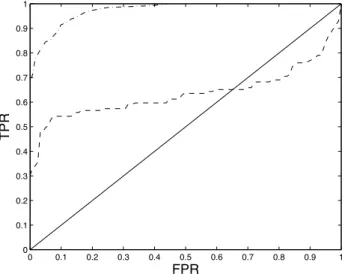
Fig. 1.ROC curves of maximum likelihood MLP (dashed-dotted line) and logistic regression (dashed line) classifiers. Curves traced out by varying costs. The ROC corresponding to random allocation is shown as the diagonal line.
degree of freedom in the binary cost matrix and, as might be expected, the entire range of classification rates for each class is swept out as the classifica-tion thresholdtvaries from 0 to 1. It is this variation of rates that the ROC curve exposes for binary classifiers. ROC analysis focuses on the classification of one particular class, sayA1,1 and plots the true positive classification rate
for A1 versus the false positive rate as the threshold t or, equivalently, the
ratio of misclassification costs is varied.
As an illustrative example we consider a two-class, two-feature synthetic data set based on a Gaussian mixture model data set introduced by Ripley [33]. Weights for the five components were (0.16,0.17,0.17,0.25,0.25): the first 3 components, with component means at (1,1)T,(−0.7,0.3)T and (0.3,0.3)T,
generateA1; while the remaining 2 components, with means at (−0.3,0.7)T
and (0.4,0.7)T, generateA
2. The covariances of all components are isotropic:
Σj = 0.03I. In the work described here 250 observations were used for
train-ing.
Figure 1 shows the ROC curve for a multi-layer perceptron (MLP) with 5 units in a single hidden layer, trained by minimising the cross entropy using quasi-Newton minimisation, which is tantamount to finding the maximum likelihood model, see for example, [3]. As illustrated by the figure, a range of true and false positive classification rates is available as the decision threshold
tis varied. The figure also shows the ROC curve for a logistic regressor [e.g. 3],
1
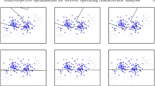
Fig. 2.Data points for an augmented version of Ripley’s synthetic data and decision boundaries of maximum likelihood classifiers at different false positive rates for the ‘circles’ class found by varying the decision thresholdt.First row:MLPs,Second row:
Logistic regression classifiers. First column: FPR = 0.04,Second column: FPR = 0.072,Third column: FPR = 0.144.
whose ROC curve is clearly inferior to the MLP’s because every point on the logistic regressor’s curve is dominated by (at least) one point on the MLP’s curve. This may be expected as the logistic regressor’s decision boundaries are constrained to be hyper-planes (straight lines in this 2D situation) and it therefore has much less flexibility than the MLP.
Figure 2 shows the decision regions for the MLP and logistic regressor when the false positive rate for the ‘circles’ class is 0.040, 0.072 and 0.144. As the figure shows the decision boundaries for the logistic regressor at different thresholds are parallel to each other because contours of posterior probability
p(Ak|x) are parallel straight lines, and there is little variation in the location
of the decision boundary as the false positive rate varies from 0.04 to 0.144. By contrast, the MLP decision boundaries are curved, better fitting the data, and the decision boundaries for different thresholds are not parallel because contours of posterior probability are not parallel. Nonetheless both sets of decision boundaries show the same general trend: a higher true positive rate is achieved by moving the decision boundary so as to encompass more A1
(circles) observations, which means that moreA2observations are erroneously
assigned as A1 resulting in an increased false positive rate.
The diagonal of the ROC plot (Figure 1) shows the performance of the classifier that allocates examples to A1 with constant probability, without
regard for the featuresx. If a classifier performs worse than random for some thresholds, such as the logistic regressor for FPR !0.63, then performance
equivalent to reflecting the ROC curve in the diagonal is obtained merely by swapping the class labels.
Portions of the logistic regressor ROC curve are markedly concave, and Scott et al. [34] and Provost and Fawcett [31, 32] have shown that classifiers with operating characteristics on the convex hull of the ROC curve can be constructed by stochastically combining classifiers on the ROC curve itself.
3.1 Pareto optimality
So far we have considered ROC curves for a single classifier as the decision thresholdt is varied. It is useful, however, to consider the classifiers that are obtained by varying, not only the decision threshold, but the classifier param-eters, such as the weights in a neural network or the thresholds in a decision tree. In general we denote these classifier parameters by w. This leads nat-urally to a multi-objective optimisation problem which may be solved using current evolutionary methods. In order to permit straightforward generali-sation to problems with more than two classes, rather than attempting to maximise the true positive rate and minimise the false positive rate, we con-sider the equivalent problem of minimising the false positive rates for both classes, which in terms of the confusion rate matrix are C12 and C21. We
therefore seek solutions to the multi-objective minimisation problem:
minimise Cjk(w,λ) for all j#=k. (5)
Here we have made explicit the dependence of the false positive rates on both the parameterswand the misclassification costsλ. For notational convenience and because they will be treated as a single entity, we write the costs and classifier parameters as a single vector of generalised parameters,θ={λ,w}; to distinguish θ from the classifier parameters w we use the optimisation terminologydecision vector to refer toθ.
If all the misclassification rates for one classifier with decision vectorθare no worse than the classification rates for another classifierφand at least one rate is better, then the classifier and costs determined byθ is said tostrictly dominate that with decision vectorφ. Thusθ strictly dominatesφ(denoted θ≺φ) iff:
Cjk(θ)≤Cjk(φ) ∀j, k and
Cjk(θ)< Cjk(φ) for some j, k. (6)
Less stringently,θ weakly dominates φ(denoted θ'φ) iff:
Cjk(θ)≤Cjk(φ) ∀j, k. (7)
A setEof decision vectors is said to be anon-dominated set if no member of the set is dominated by any other member:
A solution to the minimisation problem (5) is thusPareto optimal if it is not dominated by any other feasible solution, and the non-dominated set of all Pareto optimal solutions is known as the Pareto front. The Pareto optimal ROC curve may be thought of as the non-dominated set formed from the union of the ROC curves for each fixed parameter set w; however, multi-objective evolutionary techniques permit more efficient location of the Pareto front when the classifier has many parameters.
Recent years have seen the development of a number of evolutionary tech-niques based on dominance measures for locating the Pareto front; see [5, 6] and [36] for recent reviews. Kupinski and Anastasio [26] and Anastasio et al. [2] introduced the use of multi-objective evolutionary algorithms (MOEAs) to optimise ROC curves for binary problems, illustrating the method on a synthetic data set and for medical imaging problems; and we have used a sim-ilar methodology for locating optimal ROC curves for safety-related systems [13, 11]. In the following section we describe a straightforward evolutionary algorithm for locating the Pareto front for binary and multi-class problems. We illustrate the method on a synthetic problem for two different classifiers in Section 4.1.
4 Evolving classifiers
The algorithm we describe is based on a simple analogue of mutation-based evolution (such as [15, 13, 23, 24, 28, 27]), but any recent elitist MOEA could equally well be used [5, 6, 7, 18, 36, 38].
The algorithm, an evolution strategy (ES), maintains a set or archiveEof decision vectors, whose members are mutually non-dominating, which forms the current approximation to the Pareto front and is a source of elite solu-tions for evolution. As the computation progresses members ofEare selected, copied and their decision vectors perturbed, and the objectives corresponding to the perturbed decision vector evaluated; if the perturbed solution is not dominated by any element ofE, it is inserted intoE and any members ofE
which are dominated by the new entrant are removed. Therefore the archive can only move towards the Pareto front: it is in essence a greedy search where the archive E is the current point of the search and perturbations toE that are not dominated by the currentE are always accepted.
Algorithm 1 describes the procedure in more detail. The archive E is initialised by evaluating the misclassification rates for a number (here 100) of randomly chosen parameter values and costs, and discarding those which are dominated by another element of the initial set. Then at each generation a single element,θ is selected fromE (line 3 of Algorithm 1); selection may be uniformly random, but partitioned quasi-random selection (PQRS) [15] was used here to promote exploration of the front. PQRS prevents clustering of solutions in a particular region of the front biasing the search because they
Algorithm 1Multi-objective evolution scheme for ROC surfaces. 1:E:= initialise()
2:fort:= 1 :T Loop forT generations 3: {w,λ}=θ:= select(E) PQRS
4: w!:= perturb(w) Perturb parameters
5: fori:= 1 :L Loop over weight samples 6: λ!:= sample() Sample costs
7: C:= classify(w!,λ!) Evaluate classification rates
8: θ!:={w!,λ!}
9: ifθ!!"φ∀φ∈E
10: E:={φ∈E|φ⊀θ!}Remove dominated elements
11: E:=E∪θ! Insertθ!
12: end
13: end
14:end
are selected more frequently, thus increasing the efficiency and range of the search.
The selectedparent decision vector is copied, after which the costsλand classifier parametersw are treated separately. The parametersw of the clas-sifier are perturbed or, in the nomenclature of evolutionary algorithms, mu-tated, to form achild,w!(line 4). Here we seek to encourage wide exploration of parameter space by additively perturbing each of the parameters with a random numberδdrawn from a heavy tailed distribution (such as the Lapla-cian density, p(δ) ∝ e−|δ|). The Laplacian distribution has tails that decay relatively slowly, thus ensuring that there is a high probability of exploring regions distant from the current solutions, facilitating escape from local min-ima [37].
With a proposed parameter setw!on hand the procedure then investigates
the misclassification rates as the costs are varied with fixed parameters. In or-der to do this we generateLsample costsλ!and evaluate the misclassification rates for each of them. Since the misclassification costs are non-negative and sum to unity, a straightforward way of producing samples is to make draws from a Dirichlet distribution:
p(λ) =Dir(λ|α1, . . . ,αD) (9) = Γ( #D i=1αi) $D i=1Γ(αi) % 1− D−1 ! i=1 λi &αD−1 D−1 ' i=1 λαi−1 i (10)
where the index i labels the D ≡ Q(Q−1) off-diagonal entries in the cost matrix. Samples from a Dirichlet density lie on the simplex#
kjλkj = 1. The
αjk≥0 determine the density of the samples; since we have no preference for
particular costs here, we set all theαkj = 1 so that the simplex (that is, cost
0 0.1 0.2 0.3 0.4 0.5 0.6 0.7 0.8 0.9 1 0 0.1 0.2 0.3 0.4 0.5 0.6 0.7 0.8 0.9 1 FPR TPR
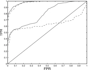
Fig. 3. ROC curves of maximum likelihood MLP (dashed-dotted line) and logis-tic regression (dashed line) classifiers, along with the optimised ROC curves for each classifier type. The ROC corresponding to random allocation is shown as the diagonal line.
The misclassification rates for each cost sampleλ! and classifier param-eters w are used to make class assignments for each example in the given dataset (line 7). Usually this step consists of merely modifying the posterior probabilitiesp(Ak|x) to find the assignment with the minimum expected cost
and is therefore computationally inexpensive as the probabilities need only be computed once for each w!. The misclassification ratesCkj(θ!) (j#=k)
com-prise the objective values for the decision vector θ! = {w!,λ} and decision vectors that are not dominated by any member of the archiveE are inserted intoE(line 11) and any decision vectors inEthat are dominated by the new entrant are removed (line 10). Since artificially limiting the archive size may inhibit convergence, the archive is permitted to grow without limit. Although managing the number of solutions in the archive has not proved a compu-tational bottleneck, data structures to efficiently maintain and query large archives may be used for very large archives [15, 22].
A (µ+λ) evolution strategy (ES) is defined as one in which µ decision vectors are selected as parents at each generation and perturbed to generate
λoffspring.2The set of offspring and parents are then truncated or replicated
to provide the µ parents for the following generation. Although Algorithm 1 is based on a (1 + 1)-ES, it is interesting to note that each parent θ is perturbed to yieldLoffspring, all of whom have the classifier parametersw!in
2
We adhere to the optimisation terminology for (µ+λ)-ES, although there is a potential for confusion with the costsλkj.
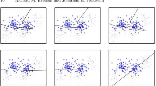
Fig. 4. Decision boundaries of optimised classifiers at different false positive rates. First row: MLPs, Second row: Logistic regression classifiers. First column:
FPR=0.04,Second column: FPR=0.072,Third column: FPR=0.144.
common. With linear costs, evaluation of the objectives for manyλ! samples is inexpensive. Nonlinear costs could be incorporated in a straightforward manner, although it would necessitate complete reclassification for each λ! sample and it would therefore be more efficient to resamplew with eachλ!.
Although we have assumed complete ignorance as to the misclassification costs, some imprecise information may often be available; for example the approximate bounds on the ratios of theλjk may be known. In this case the
evolutionary algorithm is easily focused on the relevant region by setting the Dirichlet parametersαjk appearing in (9) to be in the ratio of the expected
costs, with their magnitudes setting the variance in the cost ratios.
4.1 Illustration
Figure 3 shows the optimised ROC curve for a MLP with 5 hidden units and the optimised ROC curve for the logistic regressor, along with the origi-nal ROC curve of thesingle maximum likelihood MLP and logistic regressor classifiers from Figure 1. We emphasise that the optimised ROC curves are generally comprised of operating points for several parameter values. The ROC curve of the optimised logistic regressor is again clearly inferior to the MLP’s optimised ROC – however, the optimised ROCs are clearly superior to the ROC curves for the single maximum likelihood classifier of each family. A user is thus able to select an operating point and corresponding classifier parameters from the optimised ROC curves.
Figure 4 shows the decision regions for the optimised MLPs and logistic regressors when the false positive rateC12 is 0.040, 0.072 and 0.144. As each
point on the ROC curve may be derived from a different model parameterisa-tion as well as corresponding to different cost matrices, the decision boundaries for the logistic regressor at different thresholds are no longer parallel to each other. The MLP decision contours also show a greater difference than those from Figure 2 – again demonstrating the extra flexibility available through parameter variation. Both sets of decision boundaries again show the same general trend moving along the ROC curve from left to right, with a higher true positive rate forA1 being achieved by moving the decision boundary so
as to encompass moreA1observations and sacrificing the correct classification
ofA2 points.
4.2 Short Term Conflict Alert
As an illustration of the utility of multi-objective ROC analysis we describe its application to the optimisation of a Short Term Conflict Alert (STCA) sys-tem. This system, covering UK airspace, is responsible for providing advisory alerts to air traffic controllers if two aircraft are likely to become dangerously close. Ground-based radar is used to monitor the positions and heights of aircraft in the airspace. Having filtered out pairs of aircraft that are simply too far apart to be in any danger of collision in the next few minutes, the system makes predictions using three modules – the linear predictive filter, the current proximity filter and the manoeuvre hazard filter – whose results are combined into a final prediction. The three modules each have a number of parameters which may have different values when aircraft are in different airspace categories (for example, en route or stacked) so that w the vector describing the adjustable parameters has over 1500 entries.
Skilled staffof the National Air Traffic Services (NATS, the principal civil air traffic control authority for the UK) manually adjust ortunethese param-eters in order to reduce the number of false positive alerts while maintaining the true positive alerts. This tuning is performed manually on the basis of a database comprised of 170 000 aircraft pairs, containing historical and recent encounters. However, the receiver operating characteristics of the STCA sys-tem have been unknown, hampering the choice of the optimal operating point and parameters.
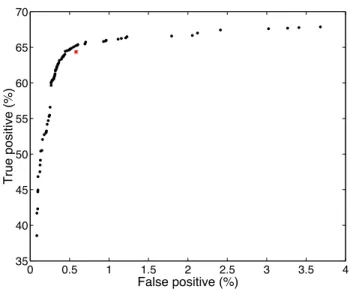
Figure 5 shows the Pareto optimal ROC front located after T = 6000 iterations of an MOEA which was permitted to adjust the 900 or so parameters that are routinely adjusted by NATS staff. The true and false positive rates corresponding to the manually tuned parameters w# are also marked as a cross. As the figure shows, the optimisation has located an ROC curve, several points of which dominate the manually tuned operating point. Although the ROC curve allows the choice of operating points that are a little better than the manually tuned operating point, we view as more important, however, the production of the ROC curve itself, because it reveals the true positive versus false positive rate trade-off, permitting a principled choice of the operating point to be made. In fact the current operating pointw#is close to the corner
0 0.5 1 1.5 2 2.5 3 3.5 4 35 40 45 50 55 60 65 70 False positive (%) True positive (%)
Fig. 5. Dots show estimates of the Pareto optimal ROC curve for STCA obtained after 6000 evaluations of a multi-objective optimiser. The cross indicates the man-ually tuned operating pointw!.
of the Pareto optimal curve. Choosing an operating point to the left of the corner would result in a rapidly diminishing true positive rate for little gain in the false positive rate; whereas operating points to the right of the corner provide small increases in the true positive rate at the expense of relatively large increases in the false positive rate.
Full details of the methods used and the results may be found in [13, 11], in which it is shown that the optimisation of the ROC curve can be carried out simultaneously with the optimisation of other objectives, for example the warning time of a possible conflict given to air traffic controllers.
5 Multi-class ROC analysis
ROC analysis for binary classification focuses on the true and false positive rates for a particular class, although the true and false positive rates for the other class are easily derived from these. However, when discriminating betweenQ > 2 classes, focussing on a single class is likely to be misleading. We consider instead the rates at which each class is misclassified into each of the other classes. With Q classes this leads us to considerD ≡Q(Q−1) misclassification ratesCkj for allj#=k. That is, we consider the off-diagonal
elements of the confusion matrix. The true positive rates, corresponding to the diagonal elements of C,are easily determined from the off-diagonal elements since each columns sums to unity. The two objective minimisation problem
for binary classification naturally generalises in the multi-class case to a D -dimensional multi-objective minimisation of the off-diagonal elements of the confusion rate matrix (5).
As in the binary classification case, the absolute magnitude of the misclas-sification costs is not important and we assume that they are normalised so that they sum to one:#
j#=kλkj = 1. There are, therefore,D−1 =Q(Q−1)−1
degrees of freedom in the cost matrix, so that the Pareto front in general has dimensionD−1 and may be thought of as a hyper-surface dividing the D -dimensional objective space of misclassification rates.
The minimisation problem (5) and Algorithm 1 were defined in such a way that they can be directly applied to the optimisation of ROC surfaces for multi-class problems, as we now illustrate.
5.1 Illustration
The synthetic data used above is simply extended to Q= 3 classes by aug-menting it with an additional Gaussian centre, so that each of the three classes is defined by a mixture of two Gaussian densities, all with isotropic covariances Σj = 0.3I. All the centres are equally weighted and ifµjifori= 1,2 denotes
the means of the two Gaussian components generating samples for class j, the centres are: µ11 = (0.7,0.3)T, µ12 = (0.3,0.3)T, µ21 = (−0.7,0.7)T,
µ22= (0.4,0.7)T,µ31= (1.0,1.0)T,µ32= (0.0,1.0)T.
We again use the MOEA to discover the Pareto optimal ROC surface for an MLP with five hidden units and softmax output units classifying 300 examples of the synthetic data. The MOEA was run for T = 10000 evalu-ations of the classifier, resulting in an estimated Pareto front or ROC sur-face comprising approximately 4800 mutually non-dominating parameter and cost combinations. The archive was initialised by training a single MLP using quasi-Newton optimisation of the data likelihood [e.g. 3] which finds a point on or near the Pareto front corresponding to equal misclassification costs; subse-quent iterations of the evolutionary algorithm are therefore largely concerned with exploring the Pareto front rather than locating it.
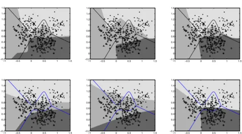
Decision regions corresponding to various places on the Pareto optimal ROC surface are shown in the top row of Figure 6. The left panel shows regions that yield the smallest total misclassification error. This point has very similar decision regions to the Bayes optimal decision regions for equal costs (equal cost decision boundaries are shown as solid lines) as may be expected since the overlap between classes is approximately comparable and there are equal numbers in each class. Note that although no explicit measures were taken to prevent over-fitting, the decision boundaries are smooth and do not show signs of over-fitting.
By contrast with decision regions that are optimal for roughly equal costs, the middle and right panels show decision regions for imbalanced costs. The middle panel shows decision regions corresponding to minimisingC21andC23:
−1 −0.5 0 0.5 1 1.5 −0.2 0 0.2 0.4 0.6 0.8 1 1.2 1.4 1.6 −1 −0.5 0 0.5 1 1.5 −0.2 0 0.2 0.4 0.6 0.8 1 1.2 1.4 1.6 −1 −0.5 0 0.5 1 1.5 −0.2 0 0.2 0.4 0.6 0.8 1 1.2 1.4 1.6 −1 −0.5 0 0.5 1 1.5 −0.2 0 0.2 0.4 0.6 0.8 1 1.2 1.4 1.6 −1 −0.5 0 0.5 1 1.5 −0.2 0 0.2 0.4 0.6 0.8 1 1.2 1.4 1.6 −1 −0.5 0 0.5 1 1.5 −0.2 0 0.2 0.4 0.6 0.8 1 1.2 1.4 1.6
Fig. 6. Decision regions for various MLPtop row and multinomial logisticbottom rowclassifiers on the multi-class ROC surface. Grey scale background shows the class to which a point would be assigned. Solid lines show the ideal equal-cost decision boundary. Symbols show actual training data.Left column:Parameters correspond-ing to minimum total misclassification error on the traincorrespond-ing data.Middle column:
Decision regions corresponding to the minimum C21 and C23 and conditioned on this, minimumC31andC13.Right column:Decision regions corresponding to min-imisingC12andC32.
everyA2example (triangles) is correctly classified, no matter what the cost.
For these data there are many parameterisations correctly classifying every
A2in the training data and we display the decision regions that also minimise
C31 and C13. For these data, it is possible to makeC31 = C13 = 0 because
A1 andA3 are adjacent only along a boundary distant fromA2points; such
complete minimisation will not be generally possible. Of course, the penalty to be paid for minimising theA2rates together withC31andC13is thatC32
andC12 are large.
The top-right panel of Figure 6 shows the reverse situation: here the costs for misclassifying eitherA1 orA3 asC2 are high. With these data, although
not in general, it is possible to reduceC12 and C32 to zero, as shown by the
decision regions which ensure thatA2examples (triangles) are only classified
correctly when it does not result in incorrect assignment of the other two classes toA2. In this case the greatest misclassification rate isC23 (triangles
as crosses).
The bottom row of Figure 6 shows decision boundaries for a multinomial logistic regressor [e.g. 3] corresponding to the same points on the Pareto opti-mal ROC surface as shown in the top row for the MLP. (The MOEA was run for 5000 generations resulting in an estimated Pareto front of approximately 9000 non-dominating cost and parameter combinations, although very similar
results are obtained after 2000 generations.) The logistic regressor is less flex-ible than an MLP, having only (d+ 1)Qparameters, wheredis the dimension of the input space. On this 2-dimensional, 3-class data it therefore has only 9 adjustable parameters (compared with the 33 for the MLP), and the decision boundaries are therefore less convoluted and less well fit to the data than those for the MLP. The same trends are evident although the classification rates are lower.
The decision regions illustrated in the middle and right columns of Figure 6 may thought of as lying on the periphery of the Pareto surface because they correspond to one or more objectives being exactly minimised. These points are the analogues of the extreme ends of the usual two-class ROC curve where the true and false positive rates for both classes are extremised. The curvature of the ROC curve in these regions is usually small, signifying that large changes in the costs yield large changes in either the true or false positive rate, but only small changes in the other. We observe a similar behaviour here: quite large changes in theλkjin these regions yield quite small changes in the all the
misclassification rates except the one which has been extremised suggesting that the curvature of the Pareto surface is low in these areas.
As we described for the STCA example, a common use of the two-class ROC curve is to locate a ‘knee’, a point of high curvature. The parameters at the knee are chosen as the operational parameters because the knee signifies the transition from rapid variation of true positive rate to rapid variation of false positive rate. A disadvantage of the multi-class ROC front is that its high dimension makes visualisation difficult, even forQ= 3 where the Pareto front is embedded in 6-dimensional space. Visualisation of these high-dimensional fronts is an area of active research; see [14] for an overview. Although, direct visualisation of the front and therefore the curvature is difficult an alternative strategy is to calculate the curvature of the manifold defined by the Pareto front and use that for selecting operating points. To date endeavours in this direction have yielded only crude approximations to the curvature even for
Q= 3 class problems and we do not present them here. However, an alterna-tive method of selecting a classifier in binary problems is to choose the one most distant from the diagonal of the ROC plot, and this idea can be naturally extended to the multi-class ROC surface, as we discuss in section 6.
As noted above, direct visualisation of the multi-class ROC surface is difficult because it is embedded in at least a 6-dimensional space. One possibility, which is explored in more depth in [10, 14], is to project the Pareto front into two or three dimensions using a data-determined nonlin-ear mapping such as Neuroscale [29] or the Self Organising Map [25] (see
http://www.dcs.ex.ac.uk/~reverson/research/mcrocfor examples). An alternative which we briefly discuss here is to project the Pareto front into false positive space. We denote byFkthe false positive rate for classk, without
0 0.5 1 0 0.2 0.4 0.6 0.8 1 0 0.5 1 F 1 F 2 F3 0 0.5 1 0 0.5 1 0 0.5 1 F 1 F2 F3 2 as 1 3 as 1 1 as 2 3 as 2 1 as 3 2 as 3
Fig. 7.The estimated Pareto front for synthetic data classified with a multinomial logistic regression classifier viewed in false positive space. Axes show the false posi-tive rates for each class and different grey scales represent the class into which the greatest number of misclassifications are made. (Points better than random shown.)
Fk(w,λ) =
!
j#=k
Ckj k= 1, . . . , Q (11)
where we emphasise the dependence of the false positive rates on the param-eterisation and costs. Each point on the Pareto front is then plotted at the coordinates given by itsQfalse positive rates. This visualisation clearly loses information on how a point is misclassified, but colour or grey scale can be utilised to indicate the class that is most misclassified. Figure 7 shows the
es-timated Pareto front for the logistic classifier visualised in this manner.3Note
that, along with all other projection methods, the projection into the lower dimensional false positive space does not preserve the mutual non-dominance between points on the front, which appears as a thickened cloud in three di-mensions. Nonetheless this sort of visualisation can be useful for navigating the Pareto front.
6 Comparing classifiers: the Gini coe
ffi
cient
In two class problems the area under the ROC curve (AUC) is often used to compare classifiers. As clearly explained by Hand and Till [19], the AUC measures a classifier’s ability to separate two classes over the range of possi-ble costs and thus be estimated using the Mann-Wilcoxon-Whitney test [19]. Unfortunately no such test is presently available for the multi-class case. The Gini coefficient is linearly related to the AUC, being twice the area between the ROC curve and the diagonal of the ROC plot. In this section we show how a natural generalisation of the Gini coefficient can be used to compare classifiers. We also draw attention to Ferri et al. [12] who give another view of the volume under multi-class ROC surfaces.
By analogy with the AUC, we might use the volume of the Q(Q− 1)-dimensional hypercube that is dominated by elements of the ROC surface for classifierAas a measure ofA’s performance. In binary and multi-class prob-lems alike its maximum value is 1 whenAclassifies perfectly. If the classifier allocates to classes at random, without regard to the features x, then the ROC surface is the simplex in Q(Q−1)-dimensional space with vertices at distanceQ−1 along each coordinate vector. The volume of the unit hypercube dominated by this simplex is [10]:
1 [Q(Q−1)]!
(
(Q−1)Q(Q−1)−Q(Q−1)(Q−2)Q(Q−1)). (12)
WhenQ= 2 this volume (area) is just 1/2,corresponding to the area under the diagonal in a conventional ROC plot.4 However, when Q >2 the volume
not dominated by the random allocation simplex is very small; even when
Q = 3, the volume not dominated is ≈0.0806. Since almost all of the unit hypercube is dominated by the random allocation simplex, we disregard this volume and instead define G(A) to be the analogue of the Gini coefficient in two dimensions, namely the proportion of the volume of the Q(Q− 1)-dimensional unit hypercube that is dominated by elements of the ROC surface,
3
The Q Fk themselves may be directly minimised, but the information on how misclassifications are made is irrecoverably lost; see also Mossman [30] who equiv-alently maximises the true positive rates.
4
Although binary ROC plots are usually made in terms of true positive rates versus false positive rates for one class, the false positive rate for the other class is just 1 minus the true positive rate for the other class.
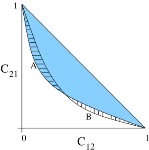
C
21C
12 0 1 1 A BFig. 8. Illustration of theG and δ measures for Q = 2. The shaded area corre-sponds to 1
2G(A), horizontal hatching indicatesδ(A, B) and vertical hatching indi-catesδ(B, A).
but is not dominated by the random allocation simplex. This is illustrated by the shaded area in Figure 8 for the Q = 2 case. In binary classification problems this corresponds to twice the area between the ROC curve and the diagonal. In multi-class problems G(A) quantifies how much better than random allocation isA. It can be simply estimated by Monte Carlo sampling of the region in the unit hypercube not dominated by the random allocation simplex.
If every point on the optimal ROC surface for classifierAis dominated by a point on the ROC surface for classifierB, then classifierBis clearly superior to classifierA. In general, however, neither ROC surface will completely dom-inate the other: regions ofA’s surfaceRA will be dominated elements ofRB
and vice versa; this corresponds to ROC curves that cross in binary problems. LetP denote the truncated pyramidal volume in the unit hypercube that is not dominated by the random allocation simplex. (In Figure 8P is the area bounded by the origin and the points (0,1) and (1,0), but when Q≥3 note that the random allocation simplex intersects the coordinate axes at (Q−1) and P is that part of the region between the simplex and the origin that also lies within the unit hypercube.) Then, to quantify the classifiers’ relative performance we defineδ(A, B) to be the volume ofP that is dominated by el-ements ofRAand not by elements ofRB (marked in Figure 8 with horizontal
lines). Note thatδ(A, B) is not a metric, because although it is non-negative, it is not symmetric. Also ifRAandRBare subsets of the same non-dominated
set W (i.e., RA ⊆W and RB ⊆W) thenδ(A, B) and δ(B, A) may have a
range of values depending on their precise composition [16]. Situations like this are rare in practice, however, and measures likeδhave proved useful for comparing Pareto fronts.
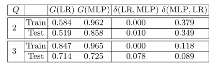
Table 1. Generalised Gini coefficients and exclusively dominated volume compar-isons of the logistic regression (LR) and MLP classifiers.
Q G(LR)G(MLP)δ(LR,MLP)δ(MLP,LR) 2 Train 0.584 0.962 0.000 0.379
Test 0.519 0.858 0.010 0.349 3 Train 0.847 0.965 0.000 0.118 Test 0.714 0.725 0.078 0.089
Table 1 shows the generalised Gini coefficient andδmeasures for the multi-nomial logistic regressor and MLP classifiers applied to the synthetic data in both the 2 and 3 class cases. The Gini coefficients indicate that both classifiers are better than random allocation and that a substantially greater volume of
P is dominated by the MLP than by the logistic regressor. Theδ measures show that, using the training data, the logistic regressor does not dominate any regions that are not dominated by the MLP, although on the test set of 1000 examples the measures indicate that the logistic regressor dominates parts of the misclassification space not dominated by the MLP.
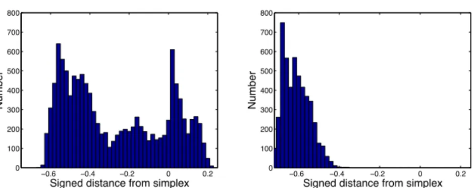
Figure 9 shows histograms of the distances from the random allocation simplex of points on the estimated Pareto fronts for the logistic regressor and MLP for the Q = 3 synthetic data. Negative distances correspond to classifiers inP, that is, closer to the origin than the random allocation simplex, while positive distances correspond to classifiers that, while non-dominated, lie beyond the random allocation simplex. These are classifiers for which a one or more misclassification rates has been allowed to become very poor in order to minimise others. As the histogram, shows the majority of classifiers are wholly better than random for both the MLP and the logistic regressor. However, the positive distances for the logistic regressor indicate that its relative inflexibility means that low misclassification rates for one class can only be achieved by sacrificing performance on others.
The distance from the random allocation simplex provides a method of se-lecting a single classifier from the Pareto front in the absence of other criteria on which to base the choice. Provided that the classifier lies within the unit hypercube, this criterion is equivalent to choosing the classifier which dom-inates the largest proportion of the region P. Figure 10 shows the decision regions for the logistic regressor and MLP corresponding to the most distant classifiers from which it can be seen that, in this case, the decision regions for these classifiers are quite close to the ideal equal-cost decision regions.
7 Conclusion
In this chapter we have considered from a multi-objective point of view the training of classifiers when the costs of misclassification are unknown. Even in
−0.6 −0.4 −0.2 0 0.2 0 100 200 300 400 500 600 700 800
Signed distance from simplex
Number −0.6 −0.4 −0.2 0 0.2 0 100 200 300 400 500 600 700 800
Signed distance from simplex
Number
Fig. 9.Distances from the random classifier simplex. Negative distances correspond to models inP.Left: Logistic regressor;Right: MLP.
Fig. 10.Decision regions for the logistic regression classifier (left) and MLP classifier (right) furthest from the random allocation simplex. Solid lines show the ideal equal-cost boundaries.
classification between two classes consideration of the costs of misclassification leads naturally to a multi-objective problem which is conventionally visualised using the receiver operating characteristic curve. The multi-objective optimi-sation framework permits the ROC curve for Q = 2 classes to be naturally generalised to a surface inQ(Q−1) dimensions in the general case. The result-ing trade-offsurface generalises the binary classification ROC curve because on it one misclassification rate cannot be improved without degrading at least one other. By viewing the classifier parameters and the misclassification costs as a single entity, we have presented a straightforward general evolutionary algorithm which is able to efficiently locate approximations to the optimal ROC surface for binary and multi-class problems alike. We remark that this algorithm is naturally able to handle other objectives (such as the warning time given to air traffic controllers in the STCA example) that the system designer must take into account.
An appealing quality of the ROC curve is that it can be plotted in two dimensions and an operating point selected from the plot. Unfortunately, the dimension of the Pareto optimal ROC surface grows as the square of the number of classes, which hampers visualisation. Projection into ‘false positive space’ is an effective visualisation method for 3-class problems as the false pos-itive rates summarise the gross overall performance, allowing further analysis of exactly which classes are misclassified into which to be focused in particular regions. We regard this method as more informative than approaches which directly minimise the false positive rates [30], and therefore ignore how mis-classifications are made. Nonetheless, it is likely that problems with more than three classes will require somea priori assessment of the important trade-offs because of the difficulty in interpreting 16 or more competing rates. Reliable calculation and visualisation of the curvature of the ROC surface is current work important for selecting operating points.
The Pareto optimal ROC surface yields a natural way of comparing clas-sifiers in terms of the volume that the clasclas-sifiers’ ROC surfaces dominate. We defined and illustrated a generalisation of the Gini index for multi-class problems that quantifies the superiority of a classifier to random allocation. This naturally leads to a criterion for selecting an operating point: choose the classifier most distant from the random allocation simplex. An alternative measure for comparing classifiers in multi-class problems is the pairwise M
measure described by Hand and Till [19]. However this describes the overall superiority of one classifier to another and does not permit selection of an operating point.
Finally we remark that the evaluation of the classification rates is inher-ently dependent on the available data. Here we have assumed that the data are of sufficient number that we can ignore any uncertainty associated with the particular data sample. Current research in this area involves bootstrapping these data in order to quantify the uncertainty in the ROC curve or surface [11] and the use of multi-objective optimisation in the presence of noise to permit reliable discovery of the Pareto optimal front with small quantities of data.
Acknowledgement
We are pleased to acknowledge support from EPSRC grant GR/R24357/01. We thank Trevor Bailey, Adolfo Hernandez, Wojtek Krzanowski, Derek Par-tridge, Vitaly Schetinin and Jufen Zhang for their helpful comments.
References
[1] N.M. Adams and D.J. Hand. Comparing classifiers when the misalloca-tion costs are uncertain. Pattern Recognition, 32:1139–1147, 1999.
[2] M. Anastasio, M. Kupinski, and R. Nishikawa. Optimization and FROC analysis of rule-based detection schemes using a multiobjective approach. IEEE Transactions on Medical Imaging, 17:1089–1093, 1998.
[3] C. Bishop. Neural Networks for Pattern Recognition. Clarendon Press, Oxford, 1995.
[4] A.P. Bradley. The use of the area under the ROC curve in the evaluation of machine learning algorithms.Pattern Recognition, 30:1145–1159, 1997. [5] C.A. Coello Coello. A Comprehensive Survey of Evolutionary-Based Mul-tiobjective Optimization Techniques. Knowledge and Information Sys-tems. An International Journal, 1(3):269–308, 1999.
[6] K. Deb. Multi-Objective Optimization Using Evolutionary Algorithms. Wiley, Chichester, 2001.
[7] K. Deb, A. Pratap, S. Agarwal, and T. Meyarivan. Fast and Elitist Mul-tiobjective Genetic Algorithm: NSGA–II. IEEE Transactions on Evolu-tionary Computation, 6(2):182–197, 2002.
[8] R.O. Duda and P.E. Hart. Pattern Classification and Scene Analysis. Wiley, New York, 1973.
[9] C. Elkan. The foundations of cost-sensitive learning. In IJCAI, pages 973–978, 2001.
[10] R.M. Everson and J.E. Fieldsend. Multi-class ROC analysis from a multi-objective optimisation perspective. Technical Report 421, Department of Computer Science, University of Exeter, April 2005.
[11] R.M. Everson and J.E. Fieldsend. Multi-objective optimisation of safety related systems: An application to short term conflict alert.IEEE Trans-actions on Evolutionary Computation, 2006. (In press).
[12] C. Ferri, J. Hern´andez-Orallo, and M.A. Salido. Volume under the ROC surface for multi-class problems. InECML 2003, pages 108–120, 2003. [13] J.E. Fieldsend and R.M. Everson. ROC Optimisation of Safety Related
Systems. In J. Hern´andez-Orallo, C. Ferri, N. Lachiche, and P. Flach, ed-itors,Proceedings of ROCAI 2004, part of the 16th European Conference on Artificial Intelligence (ECAI), pages 37–44, 2004.
[14] J.E. Fieldsend and R.M. Everson. Visualisation of multi-class ROC sur-faces. In Proceedings of the 2nd ROC Analysis in Machine Learning Workshop, part of the 22nd International Conference on Machine Learn-ing (ICML 2005), pages 49–56, 2005.
[15] J.E. Fieldsend, R.M. Everson, and S. Singh. Using Unconstrained Elite Archives for Multi-Objective Optimisation. IEEE Transactions on Evo-lutionary Computation, 7(3):305–323, 2003.
[16] J.E. Fieldsend, R.M. Everson, and S. Singh. Using Unconstrained Elite Archives for Multi-Objective Optimisation.IEEE Trans. Evol. Comp., 7 (3):305–323, 2003.
[17] P. Flach, H. Blockeel, C. Ferri, J. Hern´andez-Orallo, and J. Struyf. De-cision support for data mining: Introduction to ROC analysis and its applications. In D. Mladenic, N. Lavrac, M. Bohanec, and S. Moyle,
ed-itors,Data Mining and Decision Support: Integration and Collaboration, pages 81–90. Kluwer, 2003.
[18] C.M. Fonseca and P.J. Fleming. An Overview of Evolutionary Algorithms in Multiobjective Optimization. Evolutionary Computation, 3(1):1–16, 1995.
[19] D.J. Hand and R.J. Till. A simple generalisation of the area under the ROC curve for multiple class classification problems. Machine Learning, 45:171–186, 2001.
[20] J.A. Hanley and B.J. McNeil. The meaning and use of the area under a receiver operating characteristic (ROC) curve. Radiology, 82(143):29–36, 1982.
[21] J. Hern´andez-Orallo, C. Ferri, N. Lachiche, and P. Flach, editors. ROC Analysis in Artificial Intelligence, 1st International Workshop, ROCAI-2004, Valencia, Spain, 2004.
[22] M. T. Jensen. Reducing the Run-Time Complexity of Multiobjective EAs: The NSGA-II and Other Algorithms. IEEE Transactions on Evo-lutionary Computation, 7(5):503–515, 2003.
[23] J. Knowles and D. Corne. The Pareto Archived Evolution Strategy: A new baseline algorithm for Pareto multiobjective optimisation. In Pro-ceedings of the 1999 Congress on Evolutionary Computation, pages 98– 105, Piscataway, NJ, 1999. IEEE Service Center. URL citeseer.nj. nec.com/knowles99pareto.html.
[24] J.D. Knowles and D. Corne. Approximating the Nondominated Front Us-ing the Pareto Archived Evolution Strategy. Evolutionary Computation, 8(2):149–172, 2000.
[25] T. Kohonen. Self-Organising Maps. Springer, 1995.
[26] M.A. Kupinski and M.A. Anastasio. Multiobjective Genetic Optimiza-tion of Diagnostic Classifiers with ImplicaOptimiza-tions for Generating Receiver Operating Characterisitic Curves. IEEE Transactions on Medical Imag-ing, 18(8):675–685, 1999.
[27] M. Laumanns, L. Thiele, and E. Zitzler. Running Time Analysis of Multi-objective Evolutionary Algorithms on Pseudo-Boolean Functions. IEEE Transactions on Evolutionary Computation, 8(2):170–182, 2004.
[28] M. Laumanns, L. Thiele, E. Zitzler, E. Welzl, and K. Deb. Running Time Analysis of Multi-objective Evolutionary Algorithms on a Simple Discrete Optimization Problem. In J.J. Merelo Guerv´os, P. Adamidis, H-G Beyer, J-L Fern´andez-Villaca˜nas, and H-P Schwefel, editors, Parallel Problem Solving from Nature—PPSN VII, Lecture Notes in Computer Science, pages 44–53. Springer-Verlag, 2002.
[29] D. Lowe and M. E. Tipping. Feed-forward neural networks and topo-graphic mappings for exploratory data analysis. Neural Computing and Applications, 4:83–95, 1996.
[30] D. Mossman. Three-way ROCs. Medical Decision Making, 19(1):78–89, 1999.
[31] F. Provost and T. Fawcett. Analysis and visualisation of classifier per-formance: Comparison under imprecise class and cost distributions. In Proceedings of the Third International Conference on Knowledge Discov-ery and Data Mining, pages 43–48, Menlo Park, CA, 1997. AAAI Press. [32] F. Provost and T. Fawcett. Robust classification systems for imprecise environments. In Proceedings of the Fifteenth National Conference on Artificial Intelligence, pages 706–7, Madison, WI, 1998. AAAI Press. [33] B.D. Ripley. Neural networks and related methods for classification (with
discussion). Journal of the Royal Statistical Society Series B, 56(3):409– 456, 1994.
[34] M.J.J. Scott, M. Niranjan, and R.W. Prager. Parcel: feature sub-set selection in variable cost domains. Technical Report CUED/F-INFENG/TR.323, Cambridge University Engineering Department, 1998. [35] F. Tortorella, editor. Pattern Recognition Letters: Special Issue on ROC
Analysis in Pattern Recognition, volume 26, 2006.
[36] D. Van Veldhuizen and G. Lamont. Multiobjective Evolutionary Algo-rithms: Analyzing the State-of-the-Art.Evolutionary Computation, 8(2): 125–147, 2000.
[37] X. Yao, Y. Liu, and G. Lin. Evolutionary Programming Made Faster. IEEE Transactions on Evolutionary Computation, 3(2):82–102, 1999. [38] E. Zitzler and L. Thiele. Multiobjective Evolutionary Algorithms: A
Comparative Case Study and the Strength Pareto Approach. IEEE Transactions on Evolutionary Computation, 3(4):257–271, 1999.
[39] M.H. Zweig and G. Campbell. Receiver-operating characteristic (ROC) plots: a fundamental evaluation tool in clinical medicine. Clinical Chem-istry, 39:561–577, 1993.