Active Learning of Classification Models from Enriched Label-related Feedback
by
YanbingXue
BachelorofEngineering,ShandongUniversity,2013
Master of Science, University of Pittsburgh, 2015
Submitted to the Graduate Faculty of
the Dietrich School of Art and Science in partial fulfillment
of the requirements for the degree of
Doctor of Philosophy
Active Learning of Classification Models from Enriched Label-related Feedback Yanbing Xue, PhD
University of Pittsburgh, 2020
Our ability to learn accurate classification models from data is often limited by the number of available labeled data instances. This limitation is of particular concern when data instances need to be manually labeled by human annotators and when the labeling process carries a significant cost. Recent years witnessed increased research interest in developing methods in different directions capable of learning models from a smaller number of examples. One such direction is active learning, which finds the most informative unlabeled instances to be labeled next. Another, more recent direction showing a great promise utilizes enriched label-related feedback. In this case, such feedback from the human annotator provides additional information reflecting the relations among possible labels. The cost of such feedback is often negligible compared with the cost of instance review. The enriched label-related feedback may come in different forms. In this work, we propose, develop and study classification models for binary, multi-class and multi-label classification problems that utilize the different forms of enriched label-related feedback. We show that this new feedback can help us improve the quality of classification models compared with the standard class-label feedback. For each of the studied feedback forms, we also develop new active learning strategies for selecting the most informative unlabeled instances that are compatible with the respective feedback form, effectively combining two approaches for reducing the number of required labeled instances. We demonstrate the effectiveness of our new framework on both simulated and real-world datasets.
Keywords: active learning, classification, multi-class, multi-label, enriched label-related feedback, probabilistic score, Likert-scale feedback, ordered class set.
Table of Contents
Preface . . . xi
1.0 Introduction . . . 1
1.1 Building a classification model from human feedback . . . 2
1.1.1 Instance-based feedback . . . 4
1.1.2 Enriched-label related feedback . . . 5
1.1.3 Limitations of enriched label-related feedback . . . 7
1.2 Active learning . . . 8
1.3 Main hypothesis . . . 10
1.4 Methods developed in the thesis . . . 11
1.4.1 Learning of binary classification models from probabilistic scores and Likert-scale feedback . . . 11
1.4.2 Learning of multi-class classification models from probabilistic scores and ordered class sets . . . 12
1.4.3 Learning of multi-label classification from permutation subsets as multi-label ranking . . . 14
2.0 Background . . . 16
2.1 Binary classification learning . . . 16
2.1.1 Max-margin models . . . 17
2.1.2 Linear SVM . . . 18
2.1.3 Kernel SVM . . . 20
2.1.4 Summary . . . 22
2.2 Multi-class classification learning . . . 22
2.2.1 Multi-class support vector machine (MCSVM) . . . 23
2.2.2 Approximate multi-class support vector machine (AMSVM) . . . 24
2.2.3 Summary . . . 25
2.3.1 Binary relevance (BR) . . . 26
2.3.2 Labeling powerset (LP) . . . 27
2.3.3 Classifier chain (CC) . . . 27
2.3.4 Conditional random field (CRF) . . . 28
2.3.5 Conditional tree-structured Bayesian network (CTBN) . . . 28
2.3.6 Summary . . . 28 2.4 Learning to rank . . . 29 2.4.1 Instance ranking . . . 29 2.4.2 Label ranking . . . 30 2.4.3 Multi-label ranking . . . 30 2.4.4 Summary . . . 31
2.5 Reducing labeling efforts . . . 31
2.5.1 Active learning . . . 32
2.5.1.1 Uncertainty sampling . . . 32
2.5.1.2 Query-by-committee (QBC) . . . 33
2.5.1.3 Expectation-based strategies . . . 34
2.5.1.4 Active group learning (AGL) . . . 35
2.5.2 Learning with enriched label-related feedback . . . 35
2.5.2.1 Probabilistic scores . . . 35
2.5.2.2 Likert-scale labels . . . 37
2.5.2.3 Ordered class set (OCS) . . . 38
39 2.5.2.4 Permutationsubset . . . . 3.0 ActiveLearningof Binary Classification Models fromProbabilisticScores . . . 40
3.1 Introduction . . . 40
3.2 Methodology . . . 42
3.2.1 Problem description . . . 42
3.2.2 Method for learning with probabilistic scores . . . 42
3.2.3 Reducing the number of constraints via binning . . . 44
3.2.5 Active learning . . . 48
3.2.5.1 Expected model change . . . 48
3.2.5.2 Model change . . . 49
3.2.5.3 Distribution of ordinal categories . . . 49
3.2.5.4 Incremental training of add-one models . . . 50
3.3 Experiments and results . . . 51
3.3.1 Experiments of probabilistic scores on synthetic UCI data . . . 51
3.3.1.1 Benefit of probabilistic scores and active learning . . . 54
3.3.1.2 Effect of noise on probabilistic scores . . . 55
3.3.2 Experiments and results on time complexity . . . 56
3.3.3 Experiments of probabilistic scores on clinical data . . . 57
58 3.4 Summary . . . . 4.0 Active Learningof Binary Classification Models fromLikert-scale Feedback . . . 59
4.1 Introduction . . . 59
4.2 Methodology . . . 60
4.2.1 Problem settings . . . 60
4.2.2 Learning a classifier from Likert-scale labels . . . 61
4.2.2.1 Removing empty bins . . . 63
4.2.3 Active learning . . . 63
4.2.3.1 Expected model change . . . 63
4.2.3.2 Measuring model change . . . 64
4.2.3.3 Approximating the expectation . . . 64
4.2.3.4 Counting to preserve ordering information . . . 66
4.2.4 Training of add-one models . . . 66
4.3 Experiments and results . . . 66
4.3.1 Experiments on synthetic UCI-based data . . . 67
4.3.2 Experiments on clinical data . . . 70
5.0 Active Learningof Multi-class Classification Models
from Probabilistic Scores . . . 72
5.1 Introduction . . . 72
5.2 Methodology . . . 73
5.2.1 Multi-class support vector machine with probabilistic scores . . . 73
5.2.1.1 Problem settings . . . 73
5.2.1.2 Learning a multi-class classifier with probabilistic scores . . . 73
5.2.2 Active learning . . . 74
5.2.2.1 Expected approximate projection change . . . 75
5.2.2.2 Approximating expectation . . . 75
5.2.2.3 Approximating projection change . . . 76
5.3 Experiments and results . . . 77
5.3.1 Experiments on simulated data . . . 78
5.3.1.1 Data simulation . . . 78
5.3.1.2 Experimental settings . . . 78
5.3.1.3 Experimental results . . . 79
5.3.1.4 Noise simulation . . . 80
5.3.1.5 Experimental results with noise . . . 80
5.3.1.6 Experiments on time consumption . . . 80
5.3.2 Experiments on real-world data . . . 81
5.3.2.1 Experimental settings . . . 81
5.3.2.2 Experimental results . . . 82
82 5.4 Summary . . . . 6.0 Active Learningof Multi-class Classification Models from Ordered Class Sets . . . 84
6.1 Introduction . . . 84
6.2 Methodology . . . 85
6.2.1 Multi-class classifier with ordered class sets (OCS) . . . 86
6.2.1.1 Problem . . . 86
6.2.2 Active learning with OCS . . . 87
6.2.2.1 Expected model change (EMC) . . . 88
6.2.2.2 Estimating the probability of an unordered class set . . . 88
6.2.2.3 Estimating the conditional probability of an OCS . . . 89
6.2.2.4 Approximating the OCS change of an instance . . . 91
6.3 Experiments and results . . . 92
6.3.1 Experimental settings . . . 93
6.3.2 Experimental results . . . 95
95 6.4 Summary . . . . 7.0 Active Learningof Multi-Label Ranking, and Multi-label Classification Modelswith Permutation Subsets . . . 97
7.1 Introduction . . . 97
7.2 Methodology . . . 98
7.2.1 Problem . . . 99
7.2.2 The model . . . 99
7.2.3 An auxiliary max-margin multi-label ranker . . . 100
7.2.4 Active learning for multi-label ranking framework . . . 101
7.2.4.1 Expected model change (EMC) . . . 102
7.2.4.2 Finding the MLE of the label vector . . . 102
7.2.4.3 Estimating the conditional probability of a permutation subset . . . . 103
7.2.4.4 Approximating the change on the permutation subset of an instance . 105 7.3 Experiments and results . . . 107
7.3.1 Datasets . . . 107 7.3.2 Settings . . . 108 7.3.3 Experimental results . . . 111 7.4 Summary . . . 113 8.0 Conclusions . . . 114 8.1 Our contributions . . . 114 8.2 Open questions . . . 117 Bibliography . . . 120
List of Tables
1 Properties of all synthetic datasets in experiments. . . 68
2 Properties of two synthetic datasets in experiments. . . 80
3 Properties of all datasets (three synthetic and three real-world) in experiments. . . 93
List of Figures
1 Max-margin (support vector machines) idea. Left: many possible decisions; Right: maximum margin decision. . . 18 2 Soft-margin SVM for the linearly non-separable case. Slack variables ξi represent
distances betweenx1and margin hyperplanes. . . 19 3 Kernel SVM idea. Left: original 2D input space, positive and negative instances
are not linearly separable; Right: function φ mapping original input space to a higher-dimensional (3D) feature space, where positive and negatives can be linearly separable. . . 20 4 Relations among pairwise orderings, ordinal regression, actual and histogrammed
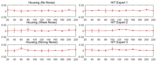
distribution on probabilistic scores (soft labels). . . 46 5 Average AUROC difference for two versions of the ordinal-regression-based method
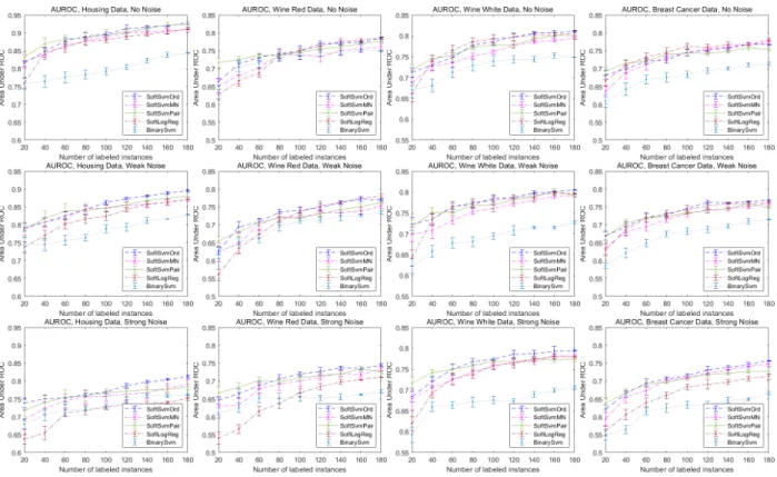
on six datasets. . . 47 6 Performance with random sampling on four synthetic datasets regarding different
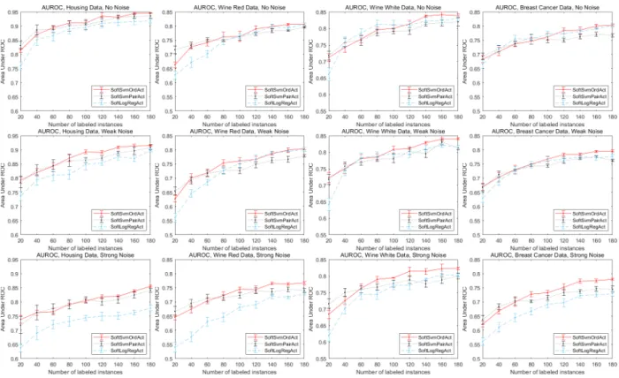
labeled instance numbers with no (top), weak (middle) and strong (bottom) noise. . . . 52 7 Performance with active learning on four synthetic datasets regarding different labeled
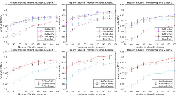
instance numbers with no (top), weak (middle) and strong (bottom) noise. . . 53 8 Performance on real-world HIT dataset annotated by three experts regarding different
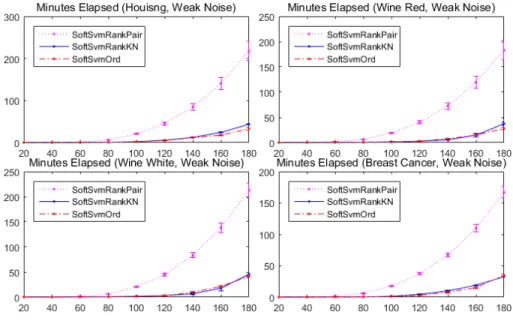
labeled instance numbers. . . 54 9 Time consumption (minutes) regarding different labeled instance numbers on four
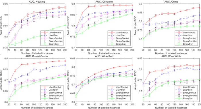
synthetic datasets with weak noise. . . 57 10 Performance regarding different labeled instance numbers on six synthetic datasets. . . 67 11 Performance on real-world HIT dataset annotated by three experts. . . 69 12 Performance (EMR) on two synthetic datasets regarding different labeled instance
numbers with no (top), weak (middle) and strong (bottom) noise. . . 78 13 Time consumption (minutes) on synthetic datasets regarding different labeled instance
14 Performance (EMR) of real-world Fact Sentiment data regarding different labeled instance numbers. . . 82 15 Performance (EMR) regarding different labeled instance numbers on two synthetic
datasets. . . 92 16 Performance (EMR) regarding different labeled instance numbers on three real-world
datasets. . . 92 17 A two-stage multi-label ranking modelfconsisting of a multi-label classifiergand an
auxiliary multi-label rankerh. . . 100 18 Performance (Micro-F1, Instance-F1, Normalized DCG) with random sampling
regarding different labeled instance numbers on all synthetic datasets. . . 109 19 Performance (Micro-F1, Instance-F1, Normalized DCG) with active learning regarding
different labeled instance numbers on all synthetic datasets. . . 110 20 Performance (Micro-F1, Instance-F1, Normalized DCG) with random sampling
regarding different labeled instance numbers on all real-world datasets. . . 111 21 Performance (Micro-F1, Instance-F1, Normalized DCG) with active learning regarding
Preface
I would like to thank everybody who made my journey to Ph.D. degree possible and joyful. First of all, I want to express my deepest gratitude to my advisor, Prof. Milos Hauskrecht, who has always supported me in both professional career and personal life. Milos taught me machine learning and data mining, and how to conduct high quality research in these fields. He also encouraged and guided me through difficult moments during my graduate school years in +Pittsburgh.
I would like to thank my thesis committee, Prof. Diane Litman, Prof. Adriana Kovashka, and Prof. Shyam Visweswaran, for their valuable feedback and discussions on my thesis research. Parts of this thesis are the results of collaboration with colleagues from University of Pittsburgh. In particular, I want to thank our fellow doctorate student, Zhipeng Luo (currently at Northwest Univ.), who helped me on several papers and gave me insights in some machine learning and optimization techniques. I also would like to thank all the other former and current members of Milos’ lab: Siqi Liu, Jeongmin Lee, Matt Barren, Dr. Charmgil Hong (currently at Handong Univ.), Dr. Zitao Liu (currently at TAL education group), Dr. Mahdi Pakdaman (currently at Microsoft), Dr. Eric Heim (currently at Carnegie Mellon Univ.), and Dr. Quang Nguyen (currently at Intuit).
I am also grateful to have many good friends in Pittsburgh, who made my life more enjoyable. In particular, I want to mention my best friend Xiaoyu Ge, who was always willing to help and gave me a lot of useful advices.
Finally, I am very grateful to my parents Wei and Shujian, my grandparents, and my cousins for their unlimited love, encouragement and support.
1.0 Introduction
In recent years, the world has witnessed a remarkable increase in the number and quality of classification models built from data. One important factor contributing to this improvement is the number of labeled data instances available to train these models. However, this improvement may not be possible when the original data are unlabeled or when the labels are obtained through additional human annotation effort. Take for example a patient’s health record. While some of the data (e.g., medications given, lab tests) are recorded, diagnoses of some conditions or adverse events that occurred during the hospitalization are not. In order to analyze and predict these conditions, individual patient instances must be first labeled by an expert. However, the process of labeling instances using subjective human assessments faces the following problem:
Collecting labels from human annotators can be extremely time-consuming and costly, especially in the domains where data assessments require a high level of expertise. In disease diagnostics, an experienced physician needs to spend about five minutes (on average) to review and evaluate one patient case [Nguyen et al., 2011a]; or in speech recognition, [Zhu, 2005] reports that a trained linguist may take up to seven hours to annotate one minute of audio record (e.g., 400 times as long). The challenge is to find ways to reduce the number of instances that need to be reviewed and labeled by an expert while improving the quality of the models learned from these instances. In this thesis, we study two complementary approaches for achieving this goal and for reducing the human annotation effort: enriched label-related feedback and active learning.
The text in the remainder of this chapter is organized as follows. We first review the different types of human feedback one can use to build classification models and introduce the enriched label-related feedback studied throughout the thesis. After that we discuss active learning strategies tailored to optimize the benefits of enriched label feedback aimed to further reduce the instance annotation cost. These two methods and their annotation benefits are the centerpieces of the main hypothesis of the thesis and its application to three classification problems: binary, multi-class and multi-label classification. Finally, we give a roadmap to the chapters of the thesis by introducing the key problems they aim to solve.
1.1 Building a classification model from human feedback
Our objective is to build a classification model. Let us assume we do not have labeled data instances to accomplish this task. What is it we can do? It is clear we need some help/feedback from a human to build a model. However, this feedback may come in different forms and with different advantages and shortcomings, say, at different cost for feedback provision. We divide the types of feedback the human experts may provide to build a classification model into three categories: (1) Model-based, (2) Instance-based, (3) Structure-based feedback.
• Model-based feedback relies on a human expert to define and build a complete classification model based on their knowledge. Typically the model is defined in some knowledge-representation language that is easy to use for a human, such as rules [Zhao et al., 2009] or decision trees [Tung, 2009]. The model-based approach expects the expert to select both the input features to use in the model and thresholds on the features. The advantage of model-based methods is their ability to handle high-dimensional data with many irrelevant features, as these are explicitly filtered out by humans. The limitation is that the burden of defining the model is squarely on the shoulders of the expert, the computational methods or tools only try to facilitate the process. Most often the hardest part of the model building process is parameter tuning. In real-world classification tasks, especially tasks with continuously numerical features, where the thresholds are not clear-cut values, the tuning of these by human experts typically requires search and iterative refinement of the model, which may significantly increase the cost.
• Instance-based feedback relies on a human to annotate a collection of prototypes used to describe the dataset. A prototype might be just one data instance, or some hypothetical instance computed from one or more of them (such as the weighted average of a set of instances). A new instance is classified by finding similar prototypes and using their classes in some way to form a prediction. In other words, human experts just need to provide the classes of some prototypes, where each prototype can be generated from one or more data instances, and the machine learning researchers are responsible to infer the implicit generalization of the dataset based on the classes of these prototypes. Enriched label-related feedback, the direction we explore in this
ability of parameter tuning. It is easy to find the optimal parameters simply by maximizing the accuracy or other desired evaluation metrics on the prototypes provided by the human experts. The main disadvantage is the amount of prototypes needed for obtaining a classification model, especially for a high-dimensional dataset. Model-based methods may eliminate the irrelevant features simply from the knowledge of the human experts, while instance-based methods may require many prototypes to infer such implicit irrelevancy.
• Structure-based feedback is an eclectic category in between pure model-based and instance-based methods. We use this category to cover human feedback that is not sufficient on its own to build a classification model but can still significantly aid the process. Briefly, like model-based methods, the human experts are asked to provide the information on the classification model. However, only some properties or structures of the model, typically the correlations among relevant features and class labels, or rough values of some parameters are provided based on the knowledge of the human experts. Hence the structure-based feedback needs to be combined with other knowledge or data to complete the model building process. An example of a structure based feedback is feature-based feedback [Druck et al., 2009]. It helps the model building processes by defining and selecting the input features to use in the model. It is one of the steps in the model-based approach, and by itself, it is not sufficient to define the full classification model so it needs to be combined with other approaches and other types of feedback to finalize the model building process. The benefit of the feature feedback is that it helps to narrow down the input features to use in the model, and as a result, it is very useful when data are high-dimensional and when they include many features irrelevant for the classification task. Another example of the structure-based feedback is a methods proposed by [Collins, 2003] for part-of-speech (POS) tagging in natural language processing, where each word in a sentence is assigned a POS tag (class) indicating its grammatical role in this sentence. This method asked the human experts to provide a collection of grammar trees representing the possible structures of English sentences. The human experts are also required to provide some labeled sentences, where each word is given its actual POS tag. Based on such information, the machine learning researchers inferred the probabilistic distribution of each word belonging to different POS tags, and found the POS tag sequence of a new sentence with highest joint probability that conforms to one of the given grammar trees.
1.1.1 Instance-based feedback
The work on enriched label-related feedback explored in this thesis falls under the umbrella of instance-based methods. However, instance-based methods are still a broad category. A sub-categorization will help to better locate enriched label-related feedback in instance-based methods. Briefly, instance-based methods can be sub-categorized based on the unit where feedback is provided:
• Group-based methods ask the human expert for the aggregated feedback of a group of data instances. In other words, the feedback from the human expert is based on a group of instances, indicating the aggregation of the feedback of all instances in this group. Multiple aggregate functions have been proposed in existing works. Multiple instance learning [Zhou and Zhang, 2002, Settles et al., 2008b] learns a binary classifier from groups of instances that are labeled by human experts as positive, if at least one instance in the group is positive, otherwise, the group is negative. Learning from label proportions [Luo and Hauskrecht, 2018a, Luo and Hauskrecht, 2018b, Luo and Hauskrecht, 2019, Luo and Hauskrecht, 2020] learns a binary classifier from groups of instances that are labeled by humans with proportion estimates, that is probability (or percentage) of positive instances in a group. The main disadvantage of group-based methods is the difficulty in group definition. Clearly the number of possible groups is exponential in the number of instances. Existing methods [Luo and Hauskrecht, 2018a, Luo and Hauskrecht, 2018b] define groups as hyper-cubes aligned to the coordinate axes in the feature space.
• Grouplet-based methods ask the human expert for the ordering or similarity information of a fixed-size small group. Unlike group-based methods, the grouplets in grouplet-based methods are always of a small fixed size (typically no more than four), the human expert provide the ordering or similarity information among the instances in this grouplet rather than aggregated feedback. [Joachims, 2002] for binary classification asked human experts to provide the ordering between two instances, since the positive instances should rank superior to the negative ones. There are also methods asking human experts for similarity information on triplets or quadruplets. Similarity information on triplets includes two instances that
are similar and one instance that is dissimilar to the former two; similarity information on quadruplets includes two instances that are similar and two instances that are dissimilar. Similarity information on triplets or quadruplets was first proposed for the learning of distance metrics [Heim et al., 2015, Heim et al., 2014, Heim and Hauskrecht, 2015], however, [Zhai et al., 2019, Chen et al., 2017] applied such information into multi-class classification since similarity information on triplets or quadruplets help aggregate intra-class instances and dis-separate inter-class instances. The main disadvantage of grouplet-based methods is fallacy hidden in the premise that the ordering or similarity information among instances is easy to obtain. This premise is true in some classification tasks when the orderings or similarities are explicit (e.g. images). However, when the ordering or similarity information is implicit or the evaluation of instances requires professional backgrounds (e.g. diagnosis), obtaining such information can be extraordinarily costly since the human annotator must evaluate all the instances in the grouplet. Another disadvantage of grouplet-based methods is the grouplet number. The maximal number of grouplets isK-polynomial to the instance number (Kis the grouplet size), which may limit the scalability of grouplet-based methods.
• Individual-instance-based methods directly ask human experts for feedback on individual data instances. Traditional instance-based methods only ask for a class label, that is, the class an individual instance belongs to. However, obtaining class labels can be very costly: in real-world classification tasks, the average time consumption of obtaining one class label ranges from minutes to hours. More sophisticated instance annotation methods ask for additional information that enhances or elaborates traditional class label feedback with information related to expert’s agreement with the label. We refer to such a feedback as enriched label related feedback and it is the main focus of the study in this thesis.
1.1.2 Enriched-label related feedback
Enriched label-related feedback assumes the human expert is able to provide, in addition to the class label, also information on his/her agreement with that label. The premise is simple: an expert who reviews the instance and gives a subjective class label can often provide us with additional information, reflecting the agreement or his/her uncertainty in the label decision. For example,
in binary classification, the human can differentiate examples that clearly, weakly or marginally represent a class. It is this type of information we seek to collect and incorporate into the model building process. Please note, we expect the added cost of this feedback is small compared to the cost of instance review and class-label decision.
There are multiple forms of enriched label-related feedback in different classification scenarios. The first form of enriched label-related feedback, to our knowledge, is probabilistic scores [Nguyen et al., 2011a, Nguyen et al., 2011b, Nguyen et al., 2013] in binary classification scenarios. Basically, in addition to a subjective class label, the human expert is also asked to provide a probabilistic score with additional information, reflecting his/her agreement in the label decision. Another form of enriched label-related feedback in binary classification scenarios is the Likert-scale feedback, where the human expert directly provides the agreement of class labels as ordinal categories. For example, when obtaining a feedback from a physician on whether the patient suffers from a particular disease or not, the physician can also provide his/her agreement in the presence of the disease on a 5-point Likert-scale feedback if he/she agrees, weakly agrees, is neutral, weakly disagrees, or disagrees with the disease. Probabilistic scores are also applicable to multi-class classification scenarios. In multi-class classification tasks, each data instance is associated with one of the multiple class labels. In addition to the class label associated with this instance, the human expert is asked to provide a probabilistic score indicating the agreement to the class label. There are also other forms of enriched label-related feedback reflecting the orderings with other classes/labels. In multi-class classification scenarios, the human expert can also be asked for the alternative classes: if the human expert does not highly agree with the class label of the data instance, s/he may also provide some other classes as alternative choices. A similar form of enriched label-related feedback also exists in multi-label classification scenarios. In multi-label classification tasks, each data instance is associated with a label vector of multiple binary values: if the binary value is positive, the instance is associated with this label, and vice versa. In multi-label classification tasks, the human expert can also be asked for the total orderings of the positive labels, since the human expert may have different agreement on different positive labels of an instance even though they are all marked by the human annotator as positive.
In this thesis, we aim to explore the different forms of enriched label-related feedback above to improve the model quality while not increase the number of labeled instances. A more detailed
introduction of our completed works to handle these enriched label-related feedback can be found in Section 1.4.
1.1.3 Limitations of enriched label-related feedback
Although enriched label-related feedback provides additional information for a data instance obtained from the annotator, it still suffers from the following risks which push us to move forward with it cautiously.
First, some forms of enriched label-related feedback may also contain noise along with additional information. This typically happens when the agreement on the classes/labels are presented as exact values. For example, when the annotator provides the confidence using probabilistic scores, these probabilistic score can be inconsistent and inaccurate [Nguyen et al., 2011a]. If the classification models are overly focused on these exact values, the hidden noise may negatively limit the performance of the classification models.
Second, the cost or time consumption of obtaining enriched label-related feedback may become non-trivial if the enriched label-related feedback is defined improperly. For example, in multi-class classification scenarios, we can ask the annotator to provide the confidence of all classes for each instance. If so, the annotation cost per instance will increase drastically when the class number is large, which contradicts our assumption that enriched label-related feedback can be obtained at a trivial cost and time consumption compared with obtaining the traditional class label of this instance.
Third, the time complexity of the classification models may become intolerable if the enriched label-related feedback is utilized improperly. For example, to eliminate the risk of the noise hidden in probabilistic scores, [Nguyen et al., 2011a, Nguyen et al., 2011b] proposed a method extracting pairwise orderings among instances from the probabilistic scores. However, the number of pairwise orderings is quadratically proportional to the instance number, leading to poor scalability, which limits the deployment of this method on larger datasets.
To eliminate the risks of enriched label-related feedback, we propose different techniques in this thesis. For example, our methods incorporating probabilistic scores are focused on the ordinal categories of confidence rather than the exact values, which eliminate the risks of the noise
hidden in the probabilistic scores. These methods are also focused on the ordinal categories rather than pairwise ordering among data instances, which reduce the time complexity. In the following subsections, we give a general overview of the works related to enriched label-related feedback we have completed, including the idea of utilizing different forms of enriched label-related feedback and how to alleviate the potential risks in different classification scenarios.
1.2 Active learning
Active learning [Lewis and Gale, 1994] is one of the most popular research directions for the problem of optimizing the time and cost of labeling. In active learning, model training and data instance annotation process are interleaved. Briefly, active learning sequentially selects and labels originally unlabeled instances that are most informative and believed to have the most significant potential to improve the model. The main challenge is for this work is to propose an active learning strategy is that it is highly related to the form of the enriched label-related feedback and the classification scenario. To address the problem, we propose complementary active learning strategies for different forms of enriched label-related feedback in different classification scenarios. There are multiple ways to assess the informativeness of an unlabeled instance. Perhaps the most popular strategy is uncertainty sampling [Lewis and Gale, 1994] which finds the unlabeled instance closest to the decision boundary of the classification model. However, uncertainty sampling is incompatible with enriched label-related feedback, since enriched label-related feedback of an instance indirectly reflects the distance of this instance to the decision boundary. Another popular strategy is query-by-committee [Seung et al., 1992, Tosh and Dasgupta, 2018] that trains a committee of multiple classification models and selects the unlabeled instance on which the committee disagrees the most. The models in the committee can be acquired from different training sets via, for example, bootstrapping all data instances [Breiman, 1996]. The limitation of query-by-committee is a potential bias introduced by the trained models. There are also more sophisticated active learning strategies named expected model change (EMC) which estimates the expected change that the unlabeled instance may bring to the classification model. Briefly, the strategy calculates the change in the model by assuming an unlabeled
instance being assigned to one of the possible labels and weights the change by an estimate of its probabilistic distribution of possible labels. The first implementation of expected model change [Tong and Koller, 2000, Settles et al., 2008b] for binary classification models with merely class labels measures the model change as the change of the model parameters. However, a large change of the parameters does not necessarily imply a large change in the predictions. Therefore, such model change typically overestimates the informativeness of the unlabeled instances. Moreover, the measurement of model change is also highly dependent on the feedback. In this thesis, we propose different approaches to measure different forms of enriched label-related feedback. For Likert-scale feedback, where the agreement of the class label is represented as one of the multiple ordinal categories, the model change can be estimated via the change of all the unlabeled instances on the predicted ordinal category. This is because such change on the ordinal category can reflect the change on the output of the classification model: if the predicted ordinal category does not change, the change on the output of the classification model is also negligible. For probabilistic scores, the model change can be estimated via the change of all the unlabeled instances on the output of the classification model. The model change can be also estimated via the change of all the unlabeled instances on the predicted category if we discretize the range of the probabilistic scores into multiple ordinal categories. For the alternative class choices in multi-class classification scenarios, the model change can be estimated via the change of all the unlabeled instances on the orderings of all the classes. We also emphasize the changes on the highly ranked classes since the change on them may affect the predicted class label. Similarly, for the total orderings of positive classes in multi-label classification scenarios, the model change can be estimated via the change of all the unlabeled instances on the orderings of all the positive labels. Moreover, the change of the binary prediction of each label should also be considered: if the one label changes from positive to negative, or vice versa, this change is greater than the change on orderings and should be emphasized.
In this thesis, we aim to explore the expected model change active learning strategy and tailor such strategy to be compatible with different forms of enriched label-related feedback in different classification scenarios to improve the model quality while not increase the number of labeled instances. A more detailed introduction of our completed works on the expected model change active learning strategy for different forms of enriched label-related feedback can be found in
Section 1.4.
1.3 Main hypothesis
The main hypothesis of our work is that with enriched label-related feedback and corresponding model learning strategies, the classification models can be built more efficiently, that is, with the same number of annotated instances, our methods can build higher performing models than methods that only utilize class-label information. Moreover, we hypothesize that learning from this new type of feedback can be further improved using matching active learning strategies. Please note that the new feedback and active learning are complementary approaches, and hence, can reduce the annotation effort both individually and jointly. In this thesis, we aim to explore the following hypotheses:
H1. Data with enriched label-related feedback and active learning can reduce the annotation effort both individually and jointly in binary classification scenarios;
H2. Data with enriched label-related feedback and active learning can reduce the annotation effort both individually and jointly in multi-class classification scenarios;
H3. Data with enriched label-related feedback and active learning can reduce the annotation effort both individually and jointly in multi-label classification scenarios.
In the following section, we briefly introduce the problems and methods for enriched label-related feedback and active learning methods we have developed in this thesis to study the above hypotheses and provide pointers to the corresponding chapters in the remainder of the document.
1.4 Methods developed in the thesis
1.4.1 Learning of binary classification models from probabilistic scores and Likert-scale feedback
Binary classification scenario is where each data instance belongs to one of the two classes (typically class 0 and class 1). In binary classification scenario, the enriched label-related feedback typically comes in two forms: (1) probabilistic scores, or (2) Likert-scale feedback [Likert, 1932]. Briefly, probabilistic scores are probabilities ranging in [0,1] (both inclusive), while Likert-scale feedback defines a set of ordinal categories. These two types of information can be used to indicate the strength of agreement (or belief) in the respective class labels. For example, when obtaining feedback from a physician on whether the patient suffers from a particular disease or not, the binary true/false feedback can be refined by obtaining physician’s belief in the presence of the disease on a probabilistic score (e.g.,70%), or a 5-point Likert-scale (e.g., strongly agree) by asking if s/he agrees, weakly agrees, is neutral, weakly disagrees, or disagrees.
Existing works [Nguyen et al., 2011a, Nguyen et al., 2011b] convert the probabilistic scores and Likert-scale feedback into pairwise orderings. Such methods show good performance and robustness against the noise in probabilistic scores. However, the number of pairwise orderings is quadratically proportional to the instance number, leading to the poor scalability of these methods. [Nguyen et al., 2013] developed new a new method based on ordinal regression [Chu and Keerthi, 2005] to learn the classification model from such two types of information and demonstrate its benefits over methods based on only class-label information. This method, apart from showing good performance and robustness against the noise in probabilistic scores, is also more scalable since the number of ordering relations obtained from ordinal regression is only linearly proportional to the instance number. However, [Nguyen et al., 2013] left a key quantity, the number of ordinal categories, undetermined. In this thesis, we propose to find the optimal number of ordinal categories via Freedman-Diaconis rule [Freedman and Diaconis, 1981].
To further improve the annotation efficiency of the above methods we enhance them with active learning strategies specifically tailored to the feedback they work with. Briefly, we propose an expected model change (EMC) [Tong and Koller, 2000, Settles et al., 2008b] active learning
strategy for both probabilistic scores and Likert-scale feedback. Such a strategy estimates the expected change of the predictions from all the add-one models of an unlabeled example. An add-one model of the unlabeled example is the model where adding this unlabeled example and a presumed probabilistic score or Likert-scale label into the labeled data. We use such an expected change of the unlabeled examples to select data examples that may help the model the best. To prevent the re-training of add-one models, which is typically inefficient and required for traditional EMC strategy, we also train the add-one models incrementally from the current model, which remarkably reduces the time consumption.
The details of methods for learning binary classification models from probabilistic scores will be discussed in Chapter 3; the details of learning of binary classification models from Likert-scale feedback will be discussed in Chapter 4.
1.4.2 Learning of multi-class classification models from probabilistic scores and ordered class sets
Multi-class classification models are typically learned from annotated data in which every data instance is associated with one class label indicating the top class choice assigned to it from among multiple classes (more than two) by a human annotator. In the multi-class classification scenario, the enriched label-related feedback can come in two forms (1) a probabilistic score, or (2) an ordered class set (OCS).
The probabilistic scores are similar to those used in the binary classification scenario. However, the ordered class sets are much different: human annotators can often express and provide additional information about the top class and its relation to other class choices. For example, when the annotation of a data instance is not a clearcut case, there are other likely class choices the annotator may have in mind. Associating multiple competing classes with one instance is common in various diagnostic tasks. For example, in the medical domain, a list of competing diagnostic classes is referred to as a differential diagnosis. Briefly, given the features (symptoms, observations, etc.) of a patient, the physician considers not only the leading diagnosis (class) but also other alternative diagnoses (classes) that are possible and may fit the patient’s case. More specifically, apart from the top class label for each data instance, we let the annotator also provide
information about other alternative classes, and express their descending priorities (or confidence) in the ordered set of classes.
Existing works [Nguyen et al., 2011a, Nguyen et al., 2011b, Nguyen et al., 2013] learning from probabilistic scores are only applicable for binary classification tasks. In this thesis, for the probabilistic scores, we use similar techniques in Section 1.4.1 based on ordinal regression [Chu and Keerthi, 2005]. OCS is a new form of enriched label-related feedback in multi-class classification tasks. To our knowledge, the work in this thesis is the first work utilizing such feedback. We build our methods for utilizing OCS in the learning process by splitting each OCS into two subsets: the subset with higher priority and the one with lower priority. Then we extract ranking information [Joachims, 2002, Herbrich et al., 1999] between these two subsets and incorporate them into approximate multi-class support vector machine (AMSVM) [He et al., 2012]. Our methods, apart from showing a good performance and robustness against the noise in probabilistic scores, is also more scalable since the number of ordering relations obtained is only linearly proportional to the instance number and to the class number.
Similarly to the binary classification problem, we aim to enhance the multi-class classification learning also with active learning methods. For the probabilistic scores, we propose an expected approximate performance change (EAPC) whose inspiration is similar to EMC in Section 1.4.1. For the ordered class sets, we propose a new variant of expected model change (EMC) [Tong and Koller, 2000, Settles et al., 2008b]. Briefly, when adding an unlabeled instance and a possible OCS of this instance into the current model, it calculates the change in the ordering induced by all one-vs-rest classifiers over all unlabeled instances. Since the OCS number of each instance is extremely large (factorial of the class space size), we also propose an approximation that subsamples the OCS’s of each unlabeled instance using t-test to find the optimal subsample size. To prevent the re-training of add-one models, which is typically inefficient and required for traditional EMC strategy, we also incorporate multiple techniques that remarkably reduce the time consumption. For EAPC for probabilistic scores, we approximate the projection change of each instance from the corresponding add-one models instead of training them. For EMC for OCS, we train the add-one models incrementally and approximate the OCS distribution by subsampling.
The details of our multi-class classification learning methods with probabilistic scores will be discussed in Chapter 5; the details of multi-class classification learning methods with OCS will be
discussed in Chapter 6.
1.4.3 Learning of multi-label classification from permutation subsets as multi-label ranking Multi-label classification models are typically learned from annotated data instances where each data instance is associated with a binary label vector, and where each scalar in the binary label vector has a0/1binary value indicating whether the data instance is relevant to this label or not. Human annotators can often provide additional information about the total orderings of the relevant labels (the labels annotated as1in the label vector) apart from the label vector itself. For example, when the relevant labels of a data instance are of different certainties, the annotator may provide such information via a permutation subset, which is useful for learning. Such permutation subset of a data instance indicates the annotator’s certainties towards the relevant labels in descending order. For example, in an image classification task, the annotator may be certain that there is a house in the image, while s/he may not be so certain whether there is also a dog, because the dog in the image is fuzzy and hard to recognize.
The learning of multi-label classification models from permutation subsets is identical to the learning of multi-label ranking models: multi-label ranking is a learning problem where the goal is to not only identify relevant labels from a set of predefined labels, but also to rank them according to their relevance to a data instance. Consequently, multi-label ranking can be considered as a generalization of multi-label classification and label ranking. Therefore, the key to learning a successful multi-label ranking model is the capture of the dependencies among the labels. However, existing works [Zhou et al., 2014, Jung and Tewari, 2018, Bucak et al., 2009] of multi-label ranking ignore the dependencies among the labels and are focused on the marginal probabilities of the labels. In this thesis, to capture the dependencies among the labels, we propose a multi-label ranking method that combines an auxiliary multi-label ranking support vector machine (MLRSVM) to effectively incorporate such permutation subsets into an existing multi-label classification model to reduce the annotation effort. We also show such auxiliary MLRSVM is a general multi-label ranking model than can be combined with any existing multi-label classification models that support gradient-based learning algorithms. Such a multi-label ranking method can also be applied to the learning of multi-label classification
models from permutation subsets. By conducting experiments on multiple datasets, our method shows it can successfully capture dependencies among labels, leading to better performance when compared with existing methods.
We propose a new active learning strategy based on the expected model change (EMC) [Tong and Koller, 2000, Settles et al., 2008b] also for the permutation subsets in the multi-label classification scenarios. Briefly, when adding an unlabeled instance and a possible permutation subset of this instance into the current model, it calculates the change in the rankings of the relevant labels overall unlabeled instances. The relevant labels are given by the existing multi-label classification model, while the rankings of the relevant labels are given by the auxiliary multi-label ranking model. Since the permutation subset number of each instance is extremely large (exponential of the label space size), we also propose an approximation that subsamples the permutation subsets of each unlabeled instance usingt-test to find the optimal subsample size. To prevent the re-training of add-one models, which is typically inefficient and required for traditional EMC strategy, we also train the add-one models incrementally and approximate the permutation subset distribution by subsampling, which remarkably reduces the time consumption.
The details of our ranking-based multi-label classification learning methods with permutation subsets will be discussed in Chapter 7.
2.0 Background
In this chapter, we outline the background and related work for the methods we describe in this thesis. We start with the basics and methods of binary classification learning, along with extension to multi-class and multi-label classification, then discuss two techniques to reduce annotation efforts: active learning and learning with enriched label-related feedback. We use the following notation throughout this thesis: matrices are denoted by capital letters, vectors by boldface lowercase letters and scalars by regular lowercase letters.
2.1 Binary classification learning
Binary learning is a sub-field of machine learning, where the task is to learn a mapping from input examples to desired 0/1outputs. In the standard binary classification setting, training data consist of examples and corresponding labels (targets), which are given by a teacher (labeler). The goal is to learn a model that can accurately predict labels of unseen future examples. Formally, given training data D = {d1, d2, . . . , dN} where di is a pair of hxi, yii, xi is an input feature
vector, yi is a desired 0/1output given by a teacher, the objective is to learn a mapping function
f : X → Y such that for a new future examplex0 , f(x0) ≈ y0. Binary classification learning has many applications in practice, for example, given data for past patients, predict whether a new patient has disease or not.
The exact form of the model f : X → Y, and the algorithms used to learn it, can take on different forms. For example, the model can be based on: logistic regression [McCullagh and Nelder, 1989], a simple (perhaps the most simple) classifier minimizing the generalization error; linear discriminant analysis (LDA) [Fisher, 1936], a mixture-of-Gaussian model performing better on unbalanced data; support vector machine (SVM) [Cortes and Vapnik, 1995, Vapnik, 1995], which formulates an optimization problem with a global optimum, and can also be adapted then applied to high-dimensional data [Hastie et al., 2009, Joachims, 1998]; naive Bayes models [Domingos and Pazzani, 1997], assuming the conditional
independence among the input features; decision trees (classification trees) [Breiman et al., 1984], creating rectangle decision boundaries among the instance; neural networks [Hastie et al., 2009, Van Der Malsburg, 1986, Rumelhart et al., 1986, Cybenko, 1989], creating different layers of neurons to achieve non-linearity, where each neuron is a simple model. In addition, there are various ensemble methods, such as bagging [Breiman et al., 1984], random forests [Ho, 1995, Ho, 1998], boosting [Schapire, 1990], and gradient boosting [Friedman, 2002, Mason et al., 2000], where multiple weak learners are combined to create a strong one.
In this section, we will describe in more detail max-margin models [Cortes and Vapnik, 1995, Vapnik, 1995, Hastie et al., 2009, Joachims, 1998] which is a widely used baseline in classification learning research. Moreover, some of our methods in this thesis are based on max-margin models so their review should help to understand them better.
2.1.1 Max-margin models
The main idea of the max-margin for classification is to find the decision hyperplane that maximizes the margin between instances of the two classes. Here “margin” is defined as the distance from the closest instances to the decision hyperplane. The intuition is that among all possible decisions, the max-margin decision has the best generalization ability. In other words, it has the best chance to classify a future instance correctly. This intuition is proved to be true. In fact, the idea has a strong foundation in statistical learning theory: [Cortes and Vapnik, 1995, Vapnik, 1995] proved that the bound on generalization error is minimized by maximizing the margin.
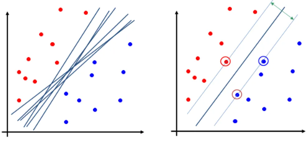
Figure 1 illustrates this idea. In Figure 1-left positive and negative examples can be perfectly separated by many linear decision boundaries. However, as argued by [Cortes and Vapnik, 1995, Vapnik, 1995], the optimal solution is the decision boundary that maximizes the margin between positive and negative examples (Figure 1-right). Note that the decision hyperplane is determined only by the examples on the margin hyperplanes (circled points in Figure 1-right). Hence, these examples are called “support vectors”. In machine learning literature, Max-margin models for classification are often referred by the term “support vector machines (SVM)”.
Figure 1: Max-margin (support vector machines) idea. Left: many possible decisions; Right: maximum margin decision.
2.1.2 Linear SVM
Now we will start with a simple case when data are linearly separable. Figure 1 illustrates a 2D example of this case. Linear SVM can be formulated by the following constrained optimization problem:
min
w,w0
R(w)
yi(wTxi+w0)≥1 ∀i= 1,2, . . . , N
whereNisthenumberofexamplesinthetrainingdata,wistheweightvectorofthemodeltobe learned. w defines the direction ofthe decision boundary. w0 is thebias term, whichdefines the shiftofthe boundary.xiandyi∈{−1,1}arefeaturevectorand label,respectively,of instancei.
R(w) is a regularization function, which is typically written in L2 norm in machine learning literature, but in general can be in L1 norm. For classification, a new instance x is assigned 1 (positive)ifwTx
i +w0 >0,otherwise-1(negative).
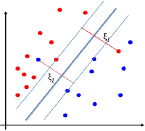
The aboveSVM formulationis calledhard-margin SVM, becauseit requiresall instancesof
Figure 2: Soft-margin SVM for the linearly non-separable case. Slack variables ξi represent
distances betweenx1 and margin hyperplanes.
data perfectly with a linear boundary, as shown in Figure 2. To handle this case, [Vapnik, 1995] relaxes the above requirement by allowing SVM to make mistakes, but mistakes are penalized in the objective function. We have the following formulation of soft-margin SVM, also called the primal form of soft-margin SVM:
min w,w0 R(w) +C N X i=1 ξi yi(wTxi+w0)≥1−ξi ∀i= 1,2, . . . , N ξi ≥0 (2.1)
Slack variablesξi represent distances betweenxiand margin hyperplanes. Note that ξi = 0if
xi is located on the correct side of the margins, otherwiseξi >0. ξi = max[0,1−yi(wTxi+w0)]
is called the hinge loss. Constant C is a trade-off parameter that defines how much misclassified examples should be penalized. In fact, hard-margin SVM is a special case of soft-margin SVM with C set to positive infinity. Therefore, further in this document, the term “Support Vector Machines” refers to soft-margin SVM.
Both hard and soft-margin formulations are convex optimization problems [Hastie et al., 2009], which means that any local optimum is also the global optimum. This
property is essential because it indicates that if we can find the best local solution, we are guaranteed to have the best global solution. This is not the case for many other classification methods (logistic regression, neural networks, etc.) [Hastie et al., 2009], where we may be “trapped” in local optima and never find the global optimum.
2.1.3 Kernel SVM
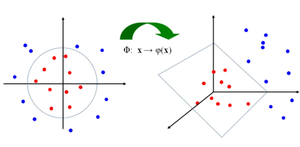
Figure 3: Kernel SVM idea. Left: original 2D input space, positive and negative instances are not linearly separable; Right: function φ mapping original input space to a higher-dimensional (3D) feature space, where positive and negatives can be linearly separable.
Linear SVM with soft margins is a powerful classifier when the non-separability is caused by a small number of outliers. However, if data are highly non-linear and are not separable by a linear boundary, e.g., data in Figure 3 (left), then Linear SVM may not perform well. This is often the problem for text and image data [Joachims, 1998]. Kernel SVM [Boser et al., 1992, Theodoridis and Koutroumbas, 2008, Joachims, 1998] was designed to solve this problem. The idea is to map features from the original space to a new higher dimensional space, where linear relations may exist. Figure 3 illustrates this idea: Figure 3-left shows positive and negative examples that cannot be separable in the 2D space; Figure 3-right shows that mappingφof input data from the original 2D space to a 3D space may introduce a linear boundary that can separate examples of two classes (in this case the linear boundary is a surface).
optimization of the following Lagrangian function: min w,w0,α L(w, w0,α) = 1 2||w|| 2 2− N X i=1 αi{yi[wTφ(xi) +w0]−1}
where α = {α1, α2, . . . , αN } is the vector of Lagrangian multipliers. Note that for the
demonstrationpurposeweuseL2normregularization||w||2,whichiswidelyusedinthemachine learningliterature.
Setting the derivatives of L(w, w0, α) with respect to w and w0 equal to 0, we obtain the followingtwoconditions:
w= N X i=1 αiyiφ(xi) 0 = N X i=1 αiyi
Plugging these conditions intoL(w, w0,α)gives the dual form of the max-margin model:
max α N X i=1 αi− 1 2 N X i,j=1 αiαjyiyjK(xi,xj) 0≥αi ≥C ∀i= 1,2, . . . , N N X i=1 αiyi = 0
whereK(xi,xj)=φ(xi)Tφ(xj)isakernelfunction.ForLinearSVM,K(xi,xj)isthedotproduct
ofxiandxj:K(xi,xj)=xi·xj.
Solving constrained optimization problems in high dimensional spaces is difficult and computationally expensive [Boseretal.,1992]. Therefore, kernel functions K(·,·) should be designedso thatSVM: (1)has therepresentationpower of highdimensional spacesand (2)still becomputationallyefficient.ThiscanbedonebychoosingamappingfromtheinputspaceX to anew featurespaceF : x → φ(x), suchthatK(xi,xj) = φ(xi)·φ(xj)wherexi,xj ∈ X. Thus,
we implicitlycompute dot productin a highdimensional spaceF, interms of operationsin the originallowdimensionalspaceX. Thisiscalledthe“kerneltrick”.
Many different types of kernels have been designed by the research community. For example, the two most widely used kernels are: (1) polynomial kernel K(xi,xj) = (c+xi ·xj)p where
p ∈ Z+is the order and c≥ 0is a constant; (2) radial basis functions (RBF) kernel K(x
i,xj) = exp(−||xi2−σ2xj||2)whereσ > 0is the standard deviation.
2.1.4 Summary
In this section, we gave a brief review of support vector machines (SVM). More details about theory and analysis of SVM can be found in [Cortes and Vapnik, 1995, Vapnik, 1995, Hastie et al., 2009, Joachims, 1998].
2.2 Multi-class classification learning
In multi-class classification models, “multi-class” indicates that the number of the classes is always greater than 2. Typically, these classes are treated equally, in other words, there is no relationship of orderings or similarities among these classes. For example, for a three-class classification model, the class labels may be represented as class 0, class 1 and class 2. Such representation of class labels may mistakenly indicate to some people that class 2 is closer to class 1 than to class 0. However, the fact is that these three classes are dissimilar with each other without any orderings. In the standard setting of multi-class classification, training data consist of examples and corresponding labels (targets), which are given by a teacher (labeler). The goal is to learn a model that can accurately predict labels of unseen future examples. Formally, given training data D = {d1, d2, . . . , dN} wheredi is a pair of hxi, yii, xi is an input feature vector, yi is a desired
categorical output given by a teacher, the objective is to learn a mapping functionf :X →Y such that for a new future examplex0 ,f(x0)≈ y0. Multi-class classification learning is also useful in practice, for example, given historical clinical data, predict which exact disease a (future) patient may have.
The exact form of the model f : X → Y, and the algorithms used to learn it can be extended from the binary classification models in Section 2.1. Some methods
for binary classification can be easily extended. For example, naive Bayes models [Domingos and Pazzani, 1997] and decision trees (classification trees) [Breiman et al., 1984] supports multi-class classification without modification, neural networks [Hastie et al., 2009, Van Der Malsburg, 1986, Rumelhart et al., 1986, Cybenko, 1989] only need to modify the output layer. In this section, we will describe multi-class support vector machine (MCSVM) [Vapnik, 1998, Weston et al., 1999] and approximate multi-class support vector machine (AMSVM) [He et al., 2012], which are two popular multi-class extensions of SVM discussed in Section 2.1.1, in more details. Briefly, these two multi-class extensions decompose the multi-class classification task into multiple binary classification tasks, and apply a binary SVM [Cortes and Vapnik, 1995, Vapnik, 1995] for each task. Also, the kernel trick for binary SVM [Hastie et al., 2009, Joachims, 1998] is compatible with these two multi-class extensions. We note, that some of our new methods presented later in the thesis are based on these methods, so a review of them should help one to understand better the following chapters of the thesis.
2.2.1 Multi-class support vector machine (MCSVM)
Our goal is to learn a multi-class classifier f : X → Y, where X is the feature space and
Y ∈ {1,2, . . . , k} represents class labels of a data instance. Hence each labeled data entry Di
consists of two components:Di =hxi, yii, an input and a class label.
In multi-class support vector machine (MCSVM), we learn k binary support vector machine jointly, one for each class. Briefly, MCSVM works by trying to assure for every training data instance the projection of its assigned class label to be higher than the projection of any other class. Therefore,(k−1)constraints are derived for each labeled data instance, one for each class, except for the assigned class label. The total number of constraints in MCSVM is thusO(kN), whereN is the number of labeled data instances. For each data instance, the projection from the binary classifier of the class label should be higher than the projection from other classes. Formally, we would like to getkprojection mappingsf1(·), f2(·), . . . , fk(·), such that for each data instance
xi, the projectionfyi(xi)is greater thanfl(xi)forl ∈ {1,2, . . . , k} \yi. To permit some flexibility, we allow violations of the constraints but penalize them through the loss function. Therefore, the multi-class support vector machine is formulated as follows:
min W,ξ 1 2 k X l=1 ||wl||22+C N X i=1 X j6=yi ξi,j (wyi −wj) Tφ(x i)≥1−ξi,j ∀i= 1,2, . . . , N ∀j 6=yi ξi,j ≥0 ∀i= 1,2, . . . , N ∀j 6=yi (2.2)
whereyiistheclasslabelofxiandφ(·)istheprojectionofkernelspace. W={w1,...,wk}are
parameters of the k binary one-vs-rest classifiers. N is thenumber of labeled instances.
Ξ = {ξ1, ξ2, . . . , ξN} are the slack variables for each constraint. For prediction, the class with
the highest projection value is selected as the predicted class.
2.2.2 Approximate multi-class support vector machine (AMSVM)
The approximate multi-class SVM (AMSVM) is an approximation of the standard multi-class SVM (MCSVM) method in Section 2.2.1. In AMSVM the set of the constraints is merged and replaced with one constraint that assumes that for each data instance the projection of the class label is higher than the average projection for all the other classes. Via such averaging, the number of constraints is significantly reduced: only one constraint is derived for each labeled data instance. Therefore, the total number of constraints in AMSVM is reduced to O(N). Formally, in the AMSVM withkclasses,kbinary SVMsf1(·), f2(·), . . . , fk(·)are trained jointly. For every
labeled instance hxi, yii, we try to assure the projection fyi(xi) of the class label yi should be greater than the average projection k−11P
l6=yifl(xi)of all the other classes l ∈ {1,2, . . . , k} \yi. The optimization of AMSVM can be formalized as:
min W,Ξ 1 2 k X l=1 ||wl||22 +C N X i=1 ξi (wyi − 1 k−1 X j6=yi wj)Tφ(xi)≥1−ξi ∀i= 1,2, . . . , N ξi ≥0 ∀i= 1,2, . . . , N (2.3)
whereyiistheclasslabelofxiandφ(·)istheprojectionofkernelspace. W={w1,...,wk}are
parameters of the k binary one-vs-rest classifiers. N is thenumber of labeled instances.
Ξ = {ξ1, ξ2, . . . , ξN} are the slack variables for each constraint. For prediction, the class with
the highest projection value is selected as the predicted class. As shown in [He et al., 2012] the performance of AMSVM is often comparable to the standard multi-class SVM (MCSVM).
2.2.3 Summary
In this section, we gave a brief review of two popular multi-class extensions of support vector machine: multi-class support vector machine (MCSVM) and approximate support vector machine (AMSVM). More details about theory and analysis of these two multi-class extensions can be found in [Vapnik, 1998, Weston et al., 1999] and [He et al., 2012] respectively.
2.3 Multi-label classification learning
In multi-label classification models, “multi-label” indicates that the number of the labels is always greater than or equal to 2. In the standard setting of multi-label classification, training data consist of data examples, and each example corresponds to a label vector of multiple binary labels (targets), which are given by a teacher (labeler). The goal is to learn a model that can accurately predict all the binary labels in the label vector of unseen future examples. Formally, given training dataD ={d(1), d(2), . . . , d(N)}whered(i)is a pair ofhx(i),y(i)i,x(i)is an input feature vector,y(i) is a desired label (output) vector of binary values given by a teacher (annotator), the objective is to learn a mapping functionf : X → Y, whereX is the feature space andY = {0,1}k represents
label vector space of a data instance, such that for a new future example x(0) , f(x(0)) ≈ y(0). Multi-label classification learning is also useful in practice, for example, given historical clinical data, predict all the diseases that a (future) patient may have.
Multi-label classification can be treated as an aggregation of multiple binary classification tasks with the same input feature vector for each data example. Multi-label classification can also be treated as an extension of multi-class classification: in multi-class classification, each instance
is associated with one single category out of all the categorical values; in multi-label classification, each instance can be associated with any number of all the categorical values.
Again, the key to learning a multi-label classification model is the successful capture of the hidden dependencies among the labels. Such hidden dependencies include the fact that some labels may typically coexist. For example, an image with beach is often with ocean as well. Such hidden dependencies also include the fact that some labels may typically be mutually exclusive. For example, an image with beach is rarely with electronics. A successful capture of the hidden dependencies helps the learning of the coexistence and mutual exclusion of the labels and can substantially improve the performance of the multi-label classification model.
The exact form of the model f : X → Y, and the algorithms used to learn it, can be directly extended from the binary classification models in Section 2.1, or the multi-class classification models in Section 2.2, or probabilistic graphical models based on directed acyclic graphs (DAGs) or undirected graphs. In this section, we will describe binary relevance (BR) [Boutell et al., 2004, Clare and King, 2001], which is directly extended from the binary classification models; labeling powerset (LP) [Tsoumakas et al., 2010], which is directly extended from the multi-class classification models; conditional random field (CRF) [Lafferty et al., 2001, Bradley and Guestrin, 2010, Naeini et al., 2015], which is extended from probabilistic graphical models based on undirected graphs (a.k.a. undirected graphical models, or UGMs); classifier chains [Read et al., 2009] and conditional tree-structured Bayesian network (CTBN) [Batal et al., 2013, Hong et al., 2014, Hong et al., 2015], which are extended from probabilistic graphical models based on DAGs (a.k.a directed graphical models, or DGMs). Although we are not deriving new methods based on these methods, some of our methods mentioned in this thesis can be combined with these methods, therefore it would be useful to have a brief introduction to them.
2.3.1 Binary relevance (BR)
Our goal is to learn a multi-label classifier f : X → Y, where X is the feature space and Y = {0,1}k represents label vector space of a data instance. Hence each labeled data entryD(i) consists of two components:D(i) =hx(i),y(i)i, an input vector and a label vector.
Binary relevance (BR) [Boutell et al., 2004, Clare and King, 2001] is a simple (perhaps the most simple) multi-label classification model that learnsk binary classifiers independently. More formally, we would like to get k binary classifiers f1(·), f2(·), . . . , fk(·) such that for new
future instance x(0), f
j(x(0)) ≈ y
(0)
j for any j ∈ {1,2, . . . , k}. Such k binary classifiers
f1(·), f2(·), . . . , fk(·) are trained independently, in other words, for any j ∈ {1,2, . . . , k}, fj(·)
is trained only onx(i)andy(i)
j fori∈ {1,2, . . . , N}.
Clearly, the limitation of binary relevance is that it totally ignores the hidden dependencies among the labels, which is the key to learning a well-performed multi-label classification model.
2.3.2 Labeling powerset (LP)
Labeling powerset (LP) [Tsoumakas et al., 2010] is another simple multi-label classification model that learns the powerset ofk labels. More formally, there are2k different outcomes for a
label vector yin the label vector spaceY = {0,1}k withk labels. Labeling powerset multi-label
classification model first constructs a one-to-one mappingg :Y ={0,1}k → Z ={1,2, . . . ,2k}
to map each outcome of a label vector into a categorical value, then learns a multi-class classifier f :X →Z such that for a new future instancex(0),f(x(0))≈g(y(0)).
Labeling powerset successfully captures the hidden dependencies among the labels by learning the full-joint of the labels. However, the limitation is also obvious: the number of the categorical values is exponential to the number of labels, which limits the scalability of this method. Also, this method cannot learn the outcomes that are absent in the label vectors of the training data.
2.3.3 Classifier chain (CC)
Classifier chain (CC) [Read et al., 2009] is a directed graphical model. Briefly, CC learns a linear chain to model the conditional likelihood over all the labels, where each label is dependent on all its former labels on the chain. More formally, we would like to obtain a decomposition of the likelihoodP(y|x) = Q
jP(yj|x, π(yj)), whereπ(yj)includes all the former labels of labelyj