Semi-parametric implied volatility surface models and forecasts based on a regression tree-boosting algorithm

Semi-parametric implied volatility surface models and

forecasts based on a regression tree-boosting algorithm

Dominik Colangelo

Submitted for the degree of Ph.D. in Economics at Swiss Finance Institute

Faculty of Economics

Universit`a della Svizzera italiana, USI Lugano, Switzerland

Thesis Committee:

Prof. F. Audrino, advisor, Universit¨at St. Gallen Prof. F. Trojani, Universit`a della Svizzera italiana Prof. W. H¨ardle, Humboldt-Universit¨at zu Berlin

Acknowledgments

I would like to thank my supervisor Prof. Francesco Audrino for his guidance throughout my doctoral studies. He taught me a lot by pushing me to my limits and beyond. This thesis is an offspring of my collaboration in his research project ‘Multivariate FGD techniques for implied volatility surfaces estimation and term structure forecasting’ that was funded by the Foundation for Research and Devel-opment of USI.

During the time spent in Lugano working at the Institute of Finance, I had the chance to make a lot of great friends, discuss my research with colleagues on numerous occasions and follow a top PhD program provided by the Swiss Finance Institute. I also discovered my own italianit`a and found the love of my life.

Special thanks and gratitude go to my wife, my parents, my sister and my extended family for their love, support and hospitality. A substantial part of the thesis has been written in the land down under.

Gabriela and Kathy take credit for proofreading, remaining typos are my sole responsibility.

Abstract

A new methodology for semi-parametric modelling of implied volatility surfaces is presented. This methodology is dependent upon the development of a feasible estimating strategy in a statistical learning framework. Given a reasonable start-ing model, a booststart-ing algorithm based on regression trees sequentially minimizes generalized residuals computed as differences between observed and estimated im-plied volatilities. To overcome the poor predicting power of existing models, a grid is included in the region of interest and a cross-validation strategy is implemented to find an optimal stopping value for the boosting procedure. Back testing the out-of-sample performance on a large data set of implied volatilities from S&P 500 options provides empirical evidence of the strong predictive power of the model. Accurate IVS forecasts also for single equity options assist in obtaining reliable trading signals for very profitable pure option trading strategies.

Contents

2 The Black-Scholes model revisited 5 2.1 GBM as a stock price process . . . 6

2.2 Pricing European plain vanilla options . . . 8

2.2.1 Ingredients of the BS framework . . . 9

2.2.2 The BS formula. . . 10

2.2.3 Comments and clarifications. . . 12

2.3 The Greeks . . . 14

2.4 No-arbitrage conditions and option bounds . . . 17

2.5 Criticism of BS framework . . . 20

3 The Implied Volatility Surface 21 3.1 Popularity of Black-Scholes IV . . . 25

3.1.1 Sublimation of model ambiguity into IV . . . 25

3.1.2 IV as an instrument for empirical option pricing . . . 25

3.1.3 IV as a risk-neutral expectation of future volatility . . . 27

3.2 Explaining the smile . . . 28

3.2.1 Deterministic instantaneous volatility . . . 28

3.2.2 Local volatility in terms of implied volatility . . . 29

3.2.3 Stochastic volatility . . . 30

3.3 Modelling IVS directly . . . 31

viii CONTENTS

3.3.1 IVS as a link to other volatility concepts. . . 31

3.3.2 Predictor space . . . 32

3.3.3 Challenges . . . 33

3.3.4 Models . . . 34

4 Supervised learning 39 4.1 Classification and regression trees . . . 41

4.2 Functional gradient descent . . . 42

5 Model and estimation procedure 47 5.1 Desired properties . . . 47

5.1.1 Improve upon a starting model . . . 48

5.1.2 Keep extremal IV in the sample . . . 51

5.1.3 Local focus . . . 53

5.1.4 OS prediction . . . 54

5.2 Inspiration . . . 55

5.3 The model. . . 57

5.4 Estimation . . . 58

5.4.1 Empirical local criterion . . . 59

5.4.2 A feasible algorithm . . . 60

6 OS analysis of the S&P 500 IVS 65 6.1 Settings . . . 66

6.1.1 Data . . . 66

6.1.2 Special days of interest. . . 71

6.1.3 Model specification . . . 71

6.1.4 Filtered historical simulation of exogenous factors . . . 78

6.1.5 OS performance measures . . . 78

6.2 Empirical results . . . 79

6.2.1 OS forecasts of predictor variables . . . 79

6.2.2 Cross-validation . . . 82

6.2.3 Relative importance of predictor variables . . . 86

6.2.4 Comparison of different models . . . 86

6.2.5 Dispersion trading . . . 90 6.2.6 Robustness check . . . 94 6.3 Summary . . . 95 7 Trading strategy 103 7.1 Settings . . . 104 7.1.1 Data . . . 104

CONTENTS ix

7.1.3 Inspiration for an option trading strategy . . . 108

7.2 Method . . . 110

7.2.1 Predicting IV changes . . . 111

7.2.2 Predicting option price changes . . . 113

7.2.3 Predicting option returns . . . 114

7.2.4 Portfolio formation . . . 115

7.3 Empirical results . . . 117

7.3.1 Portfolio return time series . . . 117

7.3.2 Sensitivity analysis . . . 123

7.3.3 Risk measures . . . 128

8 Conclusions 131 Appendices 135 A History of options 137 B Asset pricing and contingent claims 139 C Volatility 141 C.1 Instantaneous volatility . . . 142 C.2 Stochastic volatility . . . 145 C.3 Local volatility . . . 148 C.4 Implied volatility . . . 150 Bibliography 155 List of Figures 167 List of Tables 169 Abbreviations 171

Chapter 1

Introduction

The liquidity of option markets has steadily grown since the seminal work ofBlack and Scholes(1973) andMerton(1973). They showed that the price of an option is the initial cost of a self financing replicating strategy and derived the well known analytical Black-Scholes (BS) formula for European options. At the current time

t, the expiry date T, the underlying stock price St as well as the constant risk-free interest rate r are directly observable. However, the instantaneous volatility of the underlying stock return process is unknown. Using the market price of an option, it is possible to numerically solve the BS formula for the unknown volatility parameter. The resulting number is called implied volatility (IV). It is a well known empirical fact that the IV is not constant as actually assumed for deriving the BS formula. Instead, it varies over time, strike and expiry date. The concept of implied volatility surface (IVS) specifies IV as a function of moneyness

mand time to maturityτ, where the former quantifies the degree of intrinsic value in the option price and the latter the time value. m is an increasing function in the strike K, in general eventually also depending on t, T, St and r.

IV is regarded as a state variable that reflects current market situations and expections about future states. Hence it makes sense to model the IVS directly although the degenerated structure of option data makes this task difficult. Only options with a few distinct maturities, but various different strikes are traded. Certain regions of the IVS exhibit a strong dynamic that is hard to capture. A

2 CHAPTER 1. INTRODUCTION thoughtfully constructed estimation strategy needs to be considered to avoid all sorts of pitfalls (smoothness, no-arbitrage conditions, computational feasibility, overfitting, etc.).

Recently, a great deal of effort has been put into modelling the IVS directly. Gon¸calves and Guidolin (2006) combined a cross-sectional approach similar to that ofDumas, Fleming, and Whaley (1998) with vector autoregressive models. They tried, and partially succeeded depending on transaction costs, to exploit single- and multi-step ahead volatility predictions produced by their model to form profitable volatility-based trading strategies. Semi- and nonparametric smoothing methods as well as dimension-reduction techniques have also been introduced. Ski-adopoulos, Hodges, and Clewlow(2000) popularized principal components analysis (PCA) in the IVS literature. They applied PCA on a multivariate time series of IV differences for a given moneyness level and within a certain expiry range. For a surface analysis, they only used three ‘expiry buckets’ with 10 to 90, 90 to 180 and 180 to 270 days to expiry.

Cont and da Fonseca (2002) presented a functional data analysis approach based on the Karhunen-Lo`eve decomposition, an extension of the PCA method for random surfaces. Fengler, H¨ardle, and Villa(2003) argued that IVs of different maturity groups have a common eigenstructure and defined a common principal component (CPC) framework. Fengler, H¨ardle, and Mammen (2007) combined methods from functional PCA and backfitting techniques for additive models in their dynamic semiparametric factor model (dsfm). By taking the degenerated option data structure explicitly into account, they overcame some of the difficul-ties that the models based on PCA had encountered. They fitted their functional model directly on the aggregated data, without the need to estimate IV with a nonparametric smoothing estimator on a fixed grid or to sort IV into money-ness/time to expiry buckets in order to obtain a high dimensional time series of IV classes as an approximation of the IVS. In a comparison of the one-day out-of-sample prediction error, the dsfm performes only 10% better on DAX option data than a simple sticky-moneyness model, where IV is taken to be constant over time at a fixed moneyness.

1.1. GOALS 3

1.1

Goals

The first goal of this thesis is to set up a statistical learning framework that im-proves any given starting model for the IVS with an extended predictor space. The classical predictor space consisting of only m and τ is enhanced to higher dimen-sions by including a call/put dummy variable, exogenous factors and time-lagged as well as forecasted time-leading versions of themselves. Supervised learning is achieved by iteratively applying a tree-boosting algorithm.

Tree-boosting is a simple version of an optimization technique in function space called functional gradient descent (FGD), using regression trees (Breiman, Fried-man, Stone, and Olshen, 1984) as base learners and a quadratic loss function. Audrino and B¨uhlmann(2003) developed this machine learning technique for fi-nancial time series. FGD has shown its power in improving volatility forecasts in high-dimensional GARCH models for risk management purposes (Audrino and Barone-Adesi,2005), modelling interest rates (Audrino, Barone-Adesi, and Mira, 2005) and expected bond returns (Audrino and Barone-Adesi,2006). It also helps to improve the filtered historical simulation method, for example to compute re-liable out-of-sample yield curve scenarios and confidence intervals (Audrino and Trojani,2007).

The second goal is to focus on out-of-sample predictions of the IVS. For certain regions in the (m, τ) domain, the prediction errors shall be controlled such that the peformance of any reasonable starting model in forecasting IV is also improved under possible structural breaks in the time series.

The third goal is to investigate the practical use of the proposed IVS method-ology. Only a few studies link option trading with IV analysis (Ahoniemi,2006; Goyal and Saretto, 2009). This thesis defines option trading strategies and ana-lyzes their performances, also in the context of dispersion trades (Driessen, Maen-hout, and Vilkov,2009).

4 CHAPTER 1. INTRODUCTION

1.2

Outline

After thoroughly revisiting the Black-Scholes framework in Chapter 2, the related concept of implied volatility is compared in Chapter 3 to other volatility concepts that emerge from generalizing the dynamics of the underlying security. It is possi-ble to analyze the shape of the IVS for any local volatility or stochastic volatility model1_{, but the opposite direction is more promising as IV provides an exact link}

to them. Modelling the IVS directly (as a random field) raises a lot of questions about possible predictors of IVS.

Chapter 4 introduces supervised learning methods that perform automatic variable selection. Chapter 5, based on a forthcoming article in Statistics and Computing2, defines the new methodology for modelling the IVS in a statistical learning framework.

The two following chapters are empirical. In Chapter 6, the out-of-sample (OS) performance of IVS predictions for the S&P 500 index is analyzed, also for a possible application with dispersion trading. In Chapter 7, single equity option returns (the constituents of the S&P 100 index) are forecasted 10 days OS. A pure option trading strategy is defined based on that signal, relying on stability of the moneyness state during the last 20 calendar days until maturity. Conclusions are presented in Chapter 8.

1_{All such models generate an IVS with similar shape (Gatheral,2006, Chapter 7).}

2_{Audrino, F. and D. Colangelo (2009). Semi-parametric forecasts of the implied volatility}

surface using regression trees. Forthcoming inStatistics and Computing. DOI: 10.1007/s11222-009-9134-y.

Chapter 2

The Black-Scholes model

revisited

The model ofBlack and Scholes(1973) is set in a continuous-time financial market. Assume there are two securities in a frictionless market3_{, a risky asset S}

t and a risk-free securityBt that acts as a num´eraire, i.e. a saving account paying a risk-free interest rate r, here assumed to be constant and equal for borrowing and lending. The dynamics of the two securities are given by

dSt=µStdt+σStdWt (2.1)

dBt=rBtdt (2.2)

where Wt is a F-adapted standard Wiener process (a.k.a. Brownian motion) de-fined on a probability space (Ω,F,P). The filtrationFis an increasing sequence of

σ-algebras on (Ω,_F), consisting of_Ft=σ(Ws:s≤t), the smallestσ-algebra such that all _{Ws, s≤t} areFt-measurable, for t∈[0, T]. Furthermore, all P-nullsets are included inF0. In other words, the investors know the history ofS from time

0 up to present time t, but they have no information about later values.

3_{Assets are perfectly (infinitesimally) divisible, there are no short sale restrictions and no}

transaction costs occur either for buying or selling.

6 CHAPTER 2. THE BLACK-SCHOLES MODEL REVISITED

2.1

Geometric Brownian motion as a process for stock

prices

The solution of the ordinary differential equation for the num´eraire (2.2) with boundary conditionB0 = 1 is straightforward, given byBt=ert. Dividing both sides of Eq. (2.1) by St > 0 reveals that µ is the instantaneous drift and σ the instantaneous volatility of dSt/St, the percentage change process of St over an infinitesimally small period dt. Both µ and σ are assumed to be constant in the Black-Scholes (BS) framework. A process following such a stochastic differential equation (SDE) is called geometric Brownian motion (GBM). The solution to Eq. (2.1) is analytically given by St=S0exp µ₋σ 2 2 t+σWt (2.3) for any initial value S0 > 0. This can be checked with the help of Itˆo’s lemma.

For an Itˆo process of the form

Xt=X0+ Z t 0 asds+ Z t 0 bsdWs (2.4)

withapredictable and Lebesgue integrable,ba predictableW-integrable process, Itˆo’s lemma states that a twice continuously differentiable function f on Xt is itself an Itˆo process with dynamics given by

df(Xt) =f′(Xt)dXt+ 1 2f

′′_(X

t)dhXi_t, (2.5) adding half of the second derivative of f times the differential of the quadratic variation process to the standard chain rule part4. For a partition of the interval [0, t], 0 = t0 < t1 < ... < tn = t, the quadratic variation Pnk=1(Xtk −Xtk−1)

2

converges in probability to_hX_it=R₀tb2

sdsas the mesh of the partition tends to 0. Therefore, in differential notation, we havedhXit=b2tdt.

Applying Itˆo’s lemma (2.5) tof(St) = logSthelps find the solution of the SDE for a geometric Brownian motion.

4_{More generally, iff(t, X}

t) is continuously differentiable intand twice continuously

differen-tiable inXt, thendf(t, Xt) = _∂f(t,X t) ∂t dt+ ∂f(t,Xt) ∂Xt dXt +1 2 ∂2_f(t,X t) ∂X2 t dhXit.

2.1. GBM AS A STOCK PRICE PROCESS 7 dlogSt= 1 St dSt+1 2 − 1 S2 t σ2S_t2dt = 1 St (µStdt+σStdWt)− 1 2σ 2_dt = (µ₋1 2σ 2_)dt+σdW t, (2.6)

the right-hand side being independent ofSt. It follows that logSt= logS0+ (µ− 1

2σ2)t+σWt, and solving forSt leads to expression (2.3). The defining properties

of a standard Wiener process5together with the derived results imply that the log return process of St has a normal distribution,

log St Ss d ∼ N (µ−1 2σ 2_{)(t−s), σ}2_(t−s) , 0≤s < t≤T. (2.7)

Hence,St|Ss is log-normally distributed with probability density function (PDF)

ps,t(x) = 1 xb√2π exp ( −1 2 logx₋a b 2) (2.8) a:=a(s, t, µ, σ, Ss) = µ−1 2σ 2 (t−s) + logSs b:=b(s, t, σ) =σ√t−s

and cumulative distribution function (CDF) P[St≤x|Ss] =P[St≤x|Fs] = Z x 0 ps,t(y)dy (2.9) = Z logx−a b −∞ 1 √ 2π exp −1 2z 2 dz (2.10) = Z logx−a b −∞ ϕ(z)dz= Φ logx−a b . (2.11)

A change of variable takes place in (2.10),z := log_by−a. ϕ(_·) and Φ(_·) denote the PDF and CDF of a standard normal random variable.

5_{A standard Wiener process W}

t on [0, T] is defined by the following properties: W0 = 0, Wt is almost surely continuous, has independent increments and Wt−Ws

d

∼ N(0, t−s) for 0≤s < t≤T.

8 CHAPTER 2. THE BLACK-SCHOLES MODEL REVISITED The conditional expectation and variance of St|Ss under the phyiscal proba-bility measurePare

EP[St|Ss] =ea+ 1 2b2 =eµ(t−s)S_s (2.12) VarP(St|Ss) =e2a+b 2 eb2 −1 =e2µ(t−s)S_s2neσ2(t−s)₋1o. (2.13)

Remark 2.1 Note that the instantaneous drift µ is the expected percentage change in the stock price per infinitesimally small period dt, EP[dSt/St]/dt =

µ, but the expected continuously compounded return over the period [0, T] is EP h 1 T log ST S0 i =µ₋1₂σ2_.

2.2

Pricing European plain vanilla options

The term “plain vanilla option” describes the standard version of an option that does not have any special component. This is unlike an exotic option which is more complex and non-standard.

Definition 2.2 A stock option is a contract between a buyer (holder) and a seller (writer) that guarantees the buyer the right, but not the obligation, to buy (call option) or sell (put option) a share of the underlying stock at a fixed strike price

K in the future at (European-style) or up to (American-style) a fixed maturity dateT (a.k.a. expiry date). In financial jargon, the holder is said to be long and the writer short an option. If the option is exercised, the writer is obliged to fulfill the terms of the contract.

The frictionless BS financial market consisting of a risk-free security Bt =

ert with constant r and a (non-dividend paying) risky stock St that follows a geometric Brownian motion with constantµandσis complete and does not allow for arbitrage opportunities (Hafner, 2004, p. 24). A complete market is one in which any contingent claim is attainable, i.e. for any contingent claim, there exists a self-financing strategy investing in the given securities such that it replicates

2.2. PRICING EUROPEAN PLAIN VANILLA OPTIONS 9 the final value of that contingent claim. Therefore, by the fundamental theorem of asset pricing, a unique risk-neutral measure to price contingent claims exists (Schachermayer, 2009). The principles of contingent claim pricing are explained in AppendixB.

2.2.1 Ingredients of the BS framework

Equations (2.1), (2.3), (2.7) specify the stock price process and Eq. (2.8) its PDF; the pricing kernel is given by the following change of measure

dQ dP = exp ( − Z t 0 µ−r σ dWs− 1 2 Z t 0 µ−r σ 2 ds ) (2.14) and Girsanov’s theorem states that

˜ Wt= µ₋r σ t+Wt (2.15)

is a standard Brownian motion under the new measure Q, which together with Eq. (2.1) implies that the stock price process satisfies

dSt=rStdt+σStdW˜t. (2.16)

The density of Qis called risk-neutral PDF or state-price density (SPD),

qs,t(x) =dQ[St≤x|Ss] (2.17) = 1 xσp2π(t₋s)exp   − 1 2 log(_Ssx)₋ r₋₂1σ2_(t−s) σ√t₋s !2_ .

The risk-neutral PDF is Log-normal distributed like the physical PDF in Eq. (2.8), but withr instead ofµ.

The discounted stock price process ˜St = e−rtSt is a martingale under Q; to prove this, we have dS˜t = ˜StσdW˜t by virtue of Itˆo’s lemma, and an Itˆo integral is a martingale (Elliott and Kopp, 2005, Theorem 6.3.3)6. Alternatively, the

6_{The martingale representation theorem proves the converse statement. Any almost sure}

continuous martingale can be expressed as an Itˆo integral with unique integrand process w.r.t. a standard Brownian motion (Elliott and Kopp,2005, Theorem 7.3.9).

10 CHAPTER 2. THE BLACK-SCHOLES MODEL REVISITED martingale property is directly checked by

EQ[ ˜St|Fs] =S0EQ eσWt˜ −σ 2 2 t Fs (∗) = S0eσWs˜ − σ2 2 s= ˜S_s (2.18)

for all 0_≤s < t_≤T. (_∗) follows from the defining properties of a Wiener process (Elliott and Kopp,2005, Theorem 6.2.5).

According to Ait-Sahalia and Lo, “SPDs are ‘sufficient statistics’ in an eco-nomic sense – they summarize all relevant information about preferences and business conditions for purposes of pricing financial securities” (1998, p. 503). Detlefsen, H¨ardle, and Moro (2007) show how to recover the market utility func-tionU(s) implicit in the BS framework by equating the stochastic discount factor

Mt,T =βU′(ST)/U′(St) obtained in a preference-based equilibrium model, where

β is a fixed discount factor, with the state price density per unit probability

e−r(T−t)_q

t,T(ST)/pt,T(ST) that appears in the context of risk-neutral pricing. The implicit utility is a power utility of the form

U(ST) = 1₋µ−r σ2 −1 S 1−µ_σ−2r T . (2.19)

The contract specifications of a European plain vanilla stock option determine its payoff function;ψT(ST) = max(ST −K,0) for a call and ψT(ST) = max(K−

ST,0) for a put. All relevant quantities to price these contingent claims (Appendix B) have now been defined. Option prices can be obtained by calculatingπt(ψT) = EP[ψTMt,T|Ft] = EQ ψTe−r(T−t) _Ft. 2.2.2 The BS formula

Black and Scholes derive their famous option pricing formula by showing that“it is possible to create a hedged position, consisting of a long position in the stock and a short position in the [call]option [on the same stock],whose value will not depend on the price of the stock” (1973, p. 641). Since such a hedge portfolio is risk-free, its rate of return must equalr by the assumption of no-arbitrage.

dif-2.2. PRICING EUROPEAN PLAIN VANILLA OPTIONS 11 ferential equation (PDE) for the price H(t, St) of a European contingent claim7. Merton (1973) derives the BS model from weaker assumptions than in the orig-inal paper and also includes dividends. If the stock provides a dividend yield at constant rate q, then the BS PDE turns out to be

∂H ∂t + (r−q)S ∂H ∂S + 1 2σ 2_S2∂2H ∂S2 −rH = 0 (2.20)

with boundary condition H(T, ST) = ψT(ST). For European plain vanilla stock options, the solution of the PDE can be analytically calculated and is known as BS formula, CBS t =Ste−q(T−t)Φ(d1)−Ke−r(T−t)Φ(d2) (call) (2.21) PBS t =Ke−r(T−t)Φ(−d2)−Ste−q(T−t)Φ(−d1) (put) (2.22) where Φ(u) = Z u −∞ ϕ(z)dz d1 = log(St/K) + (r−q+1₂σ2)(T −t) σ√T −t ϕ(z) = √1 2πe −z2_/2 d2 =d1−σ√T −t

Definition 2.3 Thecp flag denotes a binary variable that equals 1 for a call and 0 for a put option.

The BS formula can then be written as

BSt(St, σ,cp flag, K, T, r, q) = ( CBS t ifcp flag= 1 PBS t ifcp flag= 0 . (2.23)

7_{Its payoff functionψ}

t=ψt(St) must be path-independent and a non negative random variable

that isFt-measurable. An integrability condition forψt can be found in Fengler(2005, Section

12 CHAPTER 2. THE BLACK-SCHOLES MODEL REVISITED

2.2.3 Comments and clarifications

The solution of the BS PDE (2.20) with boundary condition H(T, ST) =ψT(ST) is equivalent to the ‘linear pricing rule’ result that is inherent in the state price approach,H(t, St)≡πt(ψT(ST)). For example, the price of a European call option on a non-dividend paying stock is

Ct(St, K, T) =πt(max(ST −K,0)) =e−r(T−t)EQ[max(ST −K,0)|Ft] =e−r(T−t) Z _∞ 0 max(ST −K,0) dQ(ST|St) =e−r(T−t) Z _∞ K (ST −K)qt,T(ST) dST. (2.24)

The first part of the integral in (2.24) is

Z _∞ K STqt,T(ST) dST = EQ[ST|St]− Z K 0 STqt,T(ST) dST =er(T−t)St− Z K 0 STqt,T(ST) dST (2.25)

and the second part

Z _∞ K Kqt,T(ST) dST =KQ[ST > K|St] =K(1−Q[ST ≤K|St]) =K₋K Z K 0 qt,T(ST) dST. (2.26)

Indeed, it can be shown that

Ct(St, K, T)≡BSt(St, σ,cp flag= 1, K, T, r, q= 0).

Remark 2.4 Breeden and Litzenberger (1978) prove that qt,T(x) = dQ[ST ≤

x_|St] is the second derivative of the price of a call option with strikexat maturity

2.2. PRICING EUROPEAN PLAIN VANILLA OPTIONS 13 and the underlying portfolio may be of any type – not necessarily linear or jointly normal” (p. 649), qt,T(x) =er(T−t) ∂2_C t(St, K, T) ∂K2 K=x . (2.27)

Note 2.5 This result is only based on the specific form of the call payoff function

ψT = max(ST −K,0), as we shortly verify for Eq. (2.24) with help of Equations (2.25) and (2.26): ∂Ct(St, K, T) ∂K =e −r(T−t)Z K 0 qt,T(ST) dST −1 (2.28) ∂2Ct(St, K, T) ∂K2 =e− r(T−t)_q t,T(K). (2.29)

Remark 2.6 The BS PDE (2.20) and therefore also the BS formula (2.23) do not depend on µ. No individual investor preferences or agreements on expectations amongst investors are assumed in the BS framework.

It is quite reasonable to expect that investors may have quite differ-ent estimates for currdiffer-ent (and future) expected returns due to differdiffer-ent levels of information, techniques of analysis, etc. However, most an-alysts calculate estimates of variances and covariances in the same way: namely, by using previous price data. Since all have access to the same price history, it is also reasonable to assume that their variance-covariance estimates may be the same (Merton,1973, p. 163).

This seems to be a contradiction to the found implicit market utility (2.19). Using Eq. (2.27), Breeden and Litzenberger clarify this issue by showing that “a necessary and sufficient condition for the Black-Scholes option-pricing formula to correctly price options on aggregate consumption is that individuals’ preferences aggregate to a utility function displaying constant relative risk aversion” (1978, Theorem 3).

14 CHAPTER 2. THE BLACK-SCHOLES MODEL REVISITED

2.3

The Greeks

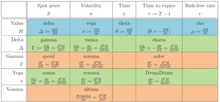
The Greeks of a European contingent claim represent the sensitivities of the value processH(t, St) to a small change in underlying parameters of the financial model. Usually, they are denoted by Greek letters. Table2.1defines the Greeks as partial derivatives ofH(t, St). The most common ones are delta, gamma, vega, theta and rho; ∆ := ∂H ∂S, Γ := ∂2_H ∂S2, ν = ∂H ∂σ, θ:= ∂H ∂t , ρ= ∂H ∂r .

The Greeks can be analytically calculated in the case of European plain vanilla stock options with given price

BSt(St, σ,cp flag, K, T, r, q) =CtBS1Icp flag=1+PtBS1Icp flag=0,

where 1Iexpression is a dummy variable that equals 1 if the expression is true and 0

otherwise. ∆BS t = ∂BSt ∂St = e−qτΦ(d1) 1Icp flag=1 +−e−qτΦ(−d1) 1Icp flag=0 (2.30) ΓBS t = ∂BSt ∂S2 t = e− qτ_ϕ(d1) Stσ√τ (2.31) νBS t = ∂BSt ∂σ =e− qτ_S t√τ ϕ(d1) (2.32) θBS t = ∂BSt ∂t = −e− qτ_S tσϕ(d1) 2√τ +qe −qτ_S tΦ(d1) −re−rτKΦ(d2) 1Icp flag=1 + −e− qτ_S tσϕ(d1) 2√τ −qe− qτ_S tΦ(−d1) +re−rτKΦ(−d2) 1Icp flag=0 (2.33) ρBS t = ∂BSt ∂r = τ e−rτKΦ(d2) 1Icp flag=1 +−τ e−rτKΦ(−d2) 1Icp flag=0 (2.34)

2 .3 . T H E G R E E K S 15

Definition of the Greeks

Spot price Volatility Time Time to expiry Risk-free rate

S σ t τ :=T −t r

Value delta vega theta rho

H ∆ := ∂H_∂S ν := ∂H_∂σ θ:= ∂H_∂t [θ=−∂H

∂τ ] ρ:= ∂H∂r

Delta gamma vanna charm

∆ Γ := ∂_∂S∆ = ∂_∂S2H2 ∂_∂σ∆ = _∂S∂ν = ∂ 2_H

∂S∂σ ∂∂τ∆ =−∂S∂θ = ∂ 2_H ∂S∂τ

Gamma speed zomma color

Γ ∂_∂SΓ = ∂_∂S3H3 ∂_∂σΓ = ∂ 3_H

∂S2_∂σ ∂_∂τΓ = ∂

3_H ∂S2_∂τ

Vega vanna vomma DvegaDtime

ν ∂_∂σ∆ = _∂S∂ν = _∂S∂σ∂2H ∂ν_∂σ = ∂_∂σ2H2 ∂ν_∂τ = ∂ 2_H ∂σ∂τ Vomma ultima ∂vomma ∂σ = ∂3_H ∂σ3

Table 2.1: “The table shows the relationship of the more common sensitivities to the four primary inputs into the Black-Scholes model (spot price of the underlying security, time remaining until option expiration, volatility and the rate of return of a risk-free investment) and to the option’s value, delta, gamma, vega and vomma. Greeks which are a first-order derivative are in [blue], second-order derivatives are in [green], and third-order derivatives are in [orange]. Note that vanna is used, intentionally, in two places as these two sensitivities are mathematically equivalent” (Wikipedia contributors,2009).

16 CHAPTER 2. THE BLACK-SCHOLES MODEL REVISITED Remark 2.7 First-order linear approximations of the loss distribution play an important role in risk management, for example when estimating the value at risk (VaR) of a stock portfolio. If the risk-factor changes have a multivariate normal distribution, then a linear combination of them is also normally distributed and it is not difficult to find the mean µp and variance σp of the portfolio. VaR is the α-quantile of the loss distribution over a specified period. In this case, the calculations simplify to VaRα =µp+σpΦ−1(α) because the normal distribution belongs to a location-scale family. Hence it is clear why this procedure is called variance-covariance method or delta-normal approach in the literature (see e.g. McNeil, Frey, and Embrechts,2005, Section 2.3.1).

For spot or forward positions in the underlying, the delta approach is fully accurate, because the associated price function . . . is linear in the underlying. The delta approximation . . . is the foundation of delta hedging: A position in the underlying asset whose size is minus the delta of the derivative is a hedge of changes in price of the derivative, if continually re-set as delta changes, and if the underlying price does not jump (Duffie and Pan,2001, Section 3.1).

Remark 2.8 Applying the delta method to an option portfolio results in a poor approximation of the true change in value because an option price is a highly nonlinear function of (t, St, σ, r, q). A better solution is given by a second-order Taylor extension. For a general portfolio value processV(t, Xt) that depends on ad-dimensional risk factor Xt, the delta-gamma method

δVt≈θδt+ ∆′δXt+ 1 2 δX

′

tΓδXt (2.35)

approximates the change in portfolio valueδVt=Vt+δt−Vtover a short fixed time

δtas a function of risk-factor changesδXt=Xt+δt−Xt. The symbol′ stands for the transpose sign. The Greeks of the portfolio areθ= ∂Vt_∂t, ∆ = [_∂Xt,∂Vt

1, . . .

∂Vt ∂Xt,d]′ (gradient) and Γ = [Γij], a d×d matrix (Hessian) with Γij = ∂

2_Vt

∂Xt,i∂Xt,j. Duffie and Pan(2001, Section 4) show how to calculate the portfolio VaR.

Remark 2.9 In his PhD thesis, Studer studied the delta-gamma method and noted that it “captures a part of the non-linearity of option portfolios. Never-theless heavy-tailedness is not included and we have the problem of estimating a

2.4. NO-ARBITRAGE CONDITIONS AND OPTION BOUNDS 17 covariance matrix [ofXt]. Finally for the last step[finding the distribution of δVt for risk management purposes]we have to rely on numerical methods(2001, p. 11). Assuming a BS framework, Studer refined the delta-gamma method in Proposi-tion 4.9 by using stochastic Taylor expansions to approximate the“distribution of the change in value of a portfolio . . . of positions in assets and derivatives in the market” (2001, p. 68).

2.4

No-arbitrage conditions and option bounds

The value of a contingent claim at expiry dateT equals its payoff, πT(ψT(ST)) =

ψT(ST) and hence it is obvious that CT(ST, K, T)−PT(ST, K, T) = max(ST −

K,0)₋max(K₋ST,0) = ST −K. A simple no-arbitrage argument shows that this equality must also hold for t < T when K is discounted appropriately, the options are of European style and the stock does not pay dividends,

Ct−Pt=St−e−r(T−t)K. (2.36)

Eq. (2.36) is calledput-call parityand is model-free, i.e. only based on the spe-cific form of European option payoff functions similar to the Breeden-Litzenberger result in Remark2.4. The put-call parity also holds for the BS formula,

CBS t =StΦ(d1)−Ke−r(T−t)Φ(d2) PBS t =Ke−r(T−t)Φ(−d2)−StΦ(−d1) ⇒CBS t −PtBS=St−Ke−r(T−t)

since Φ(di) + Φ(−di) = Φ(di) + (1−Φ(di)) = 1 for i = 1,2. If the stock pays dividends, the present value of the dividends that will be paid out before the option’s expiry dateT needs to be subtracted fromStin Eq. (2.36). If we assume a dividend yield at constant rate q, theput-call parity becomes

18 CHAPTER 2. THE BLACK-SCHOLES MODEL REVISITED

Ct, Pt ≥ 0, hence the following lower and upper bounds for European option prices are implied by Eq. (2.37):

max(e−q(T−t)St−e−r(T−t)K,0)≤Ct≤St (2.38) max(e−r(T−t)K−e−q(T−t)St,0)≤Pt ≤e−r(T−t)K. (2.39)

From Eq. (2.28) follows that ∂Ct_∂K < 0 since 0 ≤ R₀Kqt,T(ST) dST < 1 for 0_≤K <_∞ and by combining Eq. (2.28) with Eq. (2.37), we conclude that

∂Pt ∂K = ∂ Ct−e−q(T−t)St+e−r(T−t)K ∂K =e−r(T−t) Z K 0 qt,T(ST) dST >0. (2.40)

In the BS framework, a similar change of variable as in Eq. (2.11) leads to an explicit expression forQ[ST ≤K|St] since

Z K 0 qt,T(ST) dST = Φ logK₋ r₋1₂σ2_{(T −t)−logS} t σ√T₋t ! = Φ(₋d2) = 1−Φ(d2). (2.41)

The partial derivations w.r.t.K are then given by

∂CBS t ∂K =−e− r(T−t)_Φ(d 2)<0 (2.42) ∂PBS t ∂K =e −r(T−t)_{1−Φ(d 2)}>0. (2.43)

As a consequence of ∂Ct_∂K <0 and ∂Pt_∂K >0, the strike monotonicityof European options is a no-arbitrage condition: forK1 < K2 and all other variables fixed,

Ct(K1)> Ct(K2) (2.44)

Pt(K1)< Pt(K2). (2.45)

When dealing with European options on non-dividend paying stocks (q = 0), there exists amaturity monotonicity due toQ(ST1 > K|St)<Q(ST2 > K|St)

2.4. NO-ARBITRAGE CONDITIONS AND OPTION BOUNDS 19 for T1 < T2 under usual economical conditions (r > 0). In such a case, ∂Ct_∂τ =

−∂Ct∂t >0: forτ1< τ2 and all other variables fixed,

Ct(τ1)≤Ct(τ2) (2.46)

Pt(τ1)−e−rτ1K ≤Pt(τ2)−e−rτ2K. (2.47)

A long (short) butterfly spread with strikes K1 < K2 < K3 is an option strategy that is neutral in the underlying at level K2 and bearish (bullish) in

volatility, i.e. a trader taking such a position does not assume anything about the direction in whichSt moves relative toK2 ast→T (ST ≶K2?), but she believes

in decreasing (increasing) volatility such that ST is close to (far away from) K2.

A long butterfly can be created by going long 1 call with strike K1, short 2 calls with strikeK2 and long 1 call with strikeK3, all with the same maturityT, or by

doing the same with puts. The payoff function of a long butterfly is shaped like an upside-down V. There is non-zero probability that the payoff ΨT is positive, hence it must have a non-negative price by no-arbitrage:

Ct(K1)−2Ct(K2) +Ct(K3)≥0 (2.48) Pt(K1)−2Pt(K2) +Pt(K3)≥0. (2.49)

Cassese and Guidolin (2004) also discuss additional no-arbitrage conditions: reverse strike monotonicity (forK1 < K2 and all other variables fixed)

(K1−K2)e−rτ ≤Ct(K2)−Ct(K1) (2.50)

Pt(K2)−Pt(K1)≤(K2−K1)e−rτ, (2.51)

box spreads

[Pt(K2)−Ct(K2)]−[Pt(K1)−Ct(K1)] = (K2−K1)e−rτ (2.52)

and maturity spreads(for τ1< τ2 and all other variables fixed)

20 CHAPTER 2. THE BLACK-SCHOLES MODEL REVISITED Testing these no-arbitrage conditions and option price bounds empirically is rather tricky. Synchrony of option and equity prices is absolutely essential, but not necessarily ensured when using end-of-day settlement data. It is also important to mind the persistence of detected arbitrage opportunities. Market microstructure (Corsi, 2005; Bandi and Russell, 2008), transaction costs and dividends need to be taken into consideration. Put-call parity (2.37) and all derived results only hold for European options. For an overview of the classical empirical literature on testing no-arbitrage conditions in option prices seeHull (2002, Section 8.8).

2.5

Criticism of BS framework

Undoubtedly, the assumptions made in the BS framework are unrealistic. The fact that financial markets are not frictionless lies at the bottom of the market microstructure theory. A continously rebalanced hedge with or without transac-tion costs of optransac-tion positransac-tions can not be realized in practice.

“The many improvements on Black-Scholes are rarely improvements, the best that can be said for many of them is that they are just better at hiding their faults. Black-Scholes also has its faults, but at least you can see them” (Wilmott,2008).

The main flaw of the BS framework is the assumed asset price dynamics with constant volatility, only driven by independent Gaussian increments. This has led to extensive research in option pricing theory. More realistic continuous-time models and different concepts of volatility will be introduced in the next chapter.

Chapter 3

The Implied Volatility Surface

˜

σIV_{: BS}

t(St,σ˜IV,cp flag, K, T, r, q)=! Ct1Icp flag=1+Pt1Icp flag=0, (3.1)

an implied volatility (IV) can be numerically found. ˜σIV _{is unique, due to the}

monotonicity of the BS price inσ, see Eq. (2.30). According to the BS assump-tions, this implicitly calculated volatility should be constant. Cassese and Guidolin remark that “since Rubinstein (1985), it is well known that option markets are characterized by systematic deviations from the constant volatility benchmark of Black and Scholes(1973), a fact that has become even more evident after the world market crash of October 1987” (2006, p. 146).

To visualize how far BS assumptions and reality are apart, IVs for options on the S&P 500 index with different strikes K and expiry dates T are calculated on t = 10 August 2001 and plotted in Figure3.1. IV is not constant as actually assumed for deriving the BS formula. Instead, ‘smiles’ and ‘smirks’ across the

K-axis as well as a term structure along the T-axis can be seen.

22 CHAPTER 3. THE IMPLIED VOLATILITY SURFACE Implied volatilities of S&P 500 index options, t= 10 August 2001

800 1000 1200 1400 1600 1800 _{*1 *2*3} *4 *5 *6 *7 *8 0.1 0.2 0.3 0.4 0.5 0.6 0.7 0.8 0.9 1 T K IV *1 18 Aug 2001 *2 22 Sep 2001 *3 20 Oct 2001 *4 22 Dec 2001 *5 16 Mar 2002 *6 22 Jun 2002 *7 21 Dec 2002 *8 21 Jun 2003

Figure 3.1: Scatter-plot of IVs for 214 calls and 147 puts with different strikesK and expiry datesT. The underlying S&P 500 index closed at 1,190.16 points on 10 August 2001.

Definition 3.1 (IVS in absolute coordinates) The mapping ˜

σIV

t : (K, T)7−→σ˜ IV

t (K, T) (3.2)

is called the implied volatility surface (IVS) in absolute coordinates.

PluggingSt, K, r, T, and ˜σIVt (K, T) back in the BS formula leads (by definition of IV) to the observed market price. As it is usually done in the IV literature, we describe the IVS in relative coordinates.

Definition 3.2 (Relative coordinates) Moneyness is an increasing function in the strikeK, in general eventually also depending on timet, expiry dateT, the spot price of the underlying security St and risk-free interest rate r. If not stated otherwise, moneyness is defined asm=K/St throughout this thesis. τ =T−tis called time to maturity.

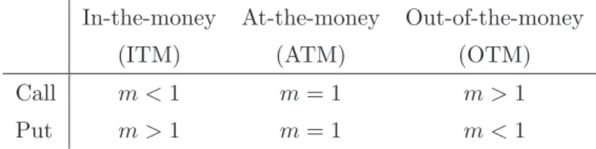
23 In-the-money At-the-money Out-of-the-money

(ITM) (ATM) (OTM)

Call m <1 m= 1 m >1

Put m >1 m= 1 m <1

Table 3.1: Moneyness categories for options when moneyness is defined asm=K/St.

They can be easily derived from relative coordinates, (K, T) = (m_·St, τ +t). At any point in time during its lifetime, an option is either in-the-money (ITM), at-the-money (ATM) or out-of-the-money (OTM).

Definition 3.3 (Intrinsic value, time value) The ITM part of the option value is called intrinsic value at time t,

max(St−K,0)1Icp flag=1+ max(K−St,0)1Icp flag=0. (3.3)

The time value is the difference between option value and intrinsic value.

The former reflects the (hypothetical) value of immediate exercise of the option and the latter the value of holding on to the option. The time value is usually decreasing as time t approaches the expiry date T. As Hull points out, “an exception to this could be an in-the-money European put option on a non-dividend-paying stock or an in-the-money European call option on a currency with a very high interest rate” (2002, p. 310). This can also be seen in the BS framework. From Eq. (2.33) follows thatθBS

t = ∂BS∂tt is not always <0 and might be positive in the aforementioned cases. A rational option holder exercises a European option atT only if its intrinsic value is positive, which implies that the option is ITM. A monyeness classification is given in Table 3.1.

Definition 3.4 (IVS in relative coordinates)

σIV t : (m, τ)7−→σ IV t (m, τ) = ˜σ IV t (m·St, t+τ) (3.4) is called the IVS in relative coordinates.

24 CHAPTER 3. THE IMPLIED VOLATILITY SURFACE Figure 3.2shows the IV plot of the earlier mentioned S&P 500 index options in relative coordinates. ‘Smiles’ and ‘smirks’ appear to form a string; although there are only a few expiry dates, a higher number of options with different strikes per string exist. This is due to institutional and practical conventions. Terms and conditions of exchange-traded options are standardized. The difference between successive expiry dates for the range of small time to maturities (τ _≤3 months) is usually one month, for large time to maturities three months. It is clear that the scatter-plot looks different on another day as IV levels, string shapes and (m, τ) location are all functions of time.

Implied volatilities of S&P 500 index options, t= 10 August 2001

0.5 1 1.5 2 0 0.5 1 1.5 2 0 0.2 0.4 0.6 0.8 1 τ m IV

Figure 3.2: IVs of S&P 500 index options on t= 10 August 2001 are plotted against relative coordinates(m, τ) = (K/St, T−t). IVs of 214callsare blue and

IVs of 147putsare red.

Definition 3.5 (Degenerated option data structure) The fact that there is only a discrete set of strikes with a small number of maturities available at each moment in time is called the degenerated structure of option data. The data is sparse and unequally distributed over the(m, τ) plane and arranged in IV strings that are moving deterministically along theτ-axis towards zero and randomly along the m-axis according to time.

3.1. POPULARITY OF BLACK-SCHOLES IV 25

3.1

Popularity of Black-Scholes implied volatility

IV, even if it is not possible to write down the function explicitly. The sufficient condition ∂BSt

∂σ 6= 0 for its existence is met because, from Eq. (2.32), it follows that the BS vega is strictly positive for call and put options, ∂CtBS

∂σ = ∂PBS

t

∂σ > 0. IV can be easily calculated with an iterative numerical procedure like the Newton-Raphson method as the BS vega is explicitely known.

3.1.1 Sublimation of model ambiguity into IV

IV as a mapping of observed option prices to volatility parameters clearly has practical advantages. “Specifying the implied volatility surface at a given date is therefore synonymous with specifying prices of all (vanilla) calls and puts at that date” (Cont and da Fonseca, 2002, p. 45). Although IV does not say anything about the ‘real’ latent instantaneous volatility per se, traders can compare op-tions with different characteristics using one single observable quantity. All model ambiguity is sublimated into σIV

t . An option with higher IV is priced relatively higher compared to another one with lower IV. Theoretically, even the option type does not play a role because put-call parity (2.36) implies equality of IV for European call and put options on the same underlying with identical strike price and maturity date.

3.1.2 IV as an instrument for empirical option pricing

Option prices can move very quickly. IV as a standardization of option prices tends to be more smooth (Shimko, 1993; Rosenberg, 2000) and less subject to noise, at least when the expiry date is τ >10 days (see Section 5.1.2). IV needs to be less frequently updated than option prices themselves. The smile curve in Figure3.2flattens out with longer time to maturity. Daglish, Hull, and Suo(2007) show that simple rules of thumb (one of them is the sticky moneyness, see Section 3.3.4) for the IVS have a reasonable one day OS prediction performance, even in

26 CHAPTER 3. THE IMPLIED VOLATILITY SURFACE cases where they are inconsistent with no-arbitrage conditions. Constraints on option prices (see Section 2.4) translate into bounds on IV. Lee(2005) describes the behaviour of IV at extreme strikes. Although the no-arbitrage conditions are quite complex, Kahal´e (2004) and Wang, Yin, and Qi (2004) are able to outline interpolation strategies. Fengler(2009) deals with the smoothing of the IVS under no-arbitrage conditions.

Benko(2006) provides a step-by-step derivation for an expression of the state-price density (2.17) in terms of IV by combining Eq. (2.23) and (2.27),

qt,T(K) =erτStϕ(d1)√τ ( 1 K2_σIV t τ +∂σ IV t ∂K 2d1 √ τ KσIV t +∂ 2_σIV t ∂K2 + ∂σIV t ∂K 2 d1d2 σIV t ) . (3.5)

Bliss and Panigirtzoglou (2002); Brunner and Hafner (2003) find that an SPD estimation inferred from the IVS can be superior to classical approaches directly based on option prices (Breeden and Litzenberger,1978;A¨ıt-Sahalia and Lo,1998; Britten-Jones and Neuberger,2000). Latest approaches focus directly on the pric-ing kernelMt,T =qt,T/pt,T, taking into account both option prices and the time series of St (Detlefsen et al., 2007; Barone-Adesi, Engle, and Mancini, 2008). Gagliardini, Gouri´eroux, and Renault (2008) obtain an estimator of Mt,T by an extended method of moments that combines no-arbitrage restrictions with IVS interpolation.

Delta hedging reduces the risk of price movements in the underlying asset. For example, a long equity call option is delta hedged by shorting ∆ = ∂Ct_∂St stocks. The portfolio value process Ht = Ct−∆St has a zero delta in this way, ∂Ht_∂St = ∂Ct

∂St − ∂Ct

∂St = 0. Practitioners often use the BS delta calibrated at the IV as hedge ratio, ∆ = ∆BS

t = ∂∂StBSt(St, σtIV,cp flag, K, T, r, q). Barone-Adesi and Elliott(2007) explain the good performance of this so called ‘IV compensated BS hedge’ with local first degree homogeneity8 ofCtw.r.t.StandK. Fengler(2005, Section 2.9.1) shows how a ‘corrected hedge ratio’ can be obtained from ∆BS

t when an explicit

8_{This property also holds for BS option prices. For a >0, BS}

t(aSt, σ,cp flag, aK, T, r, q) =

3.1. POPULARITY OF BLACK-SCHOLES IV 27 dependence of IV onStis assumed, ∆ = ∆BSt +νtBS

∂σIV

t

∂St . IVS is a function of (m, τ) and not of St, but Lee (2005) proves in a stochastic volatility framework that

∂σIV

t

∂St = −KSt ∂σIV

t

∂K . The previous examples show how different volatility concepts are connected with each other and consolidates the importance of BS IV as a building block in risk management (see Remarks2.7,2.8 and2.9).

3.1.3 IV as a risk-neutral expectation of future volatility

IV can be interpreted as the market’s expectation of average volatility through the lifetime of the option. In a BS similar framework where volatility is allowed to be a deterministic function of time only and under mild conditions (Karatzas and Shreve,1991, Theorem 5.2.9), the complete market setting is preserved and it can be shown that the fair price of European plain vanilla stock options is given by BSt St, √ ¯ σ2_{,cp flag, K, T, r, q, (3.6)}

the common BS formula (2.23) with

¯ σ2:= 1 T ₋t Z T t σ2(s)ds. (3.7)

In a general stochastic volatility setup (see AppendixC.2), whereσ(t, Yt) =f(Yt) is a function of time and an Itˆo processYtthat drives the volatility dynamics, one can show that

BSt St,EQ˜ h√ ¯ σ2_F t i ,cp flag, K, T, r, q (3.8) with ¯ σ2 := 1 T −t Z T t f(Ys)2ds (3.9)

and ˜Qa risk-neutral measure9 is only an approximation to the fair price of ATM options if additionally zero correlation between the Brownian motions in the SDE forStand the SDE forYtis assumed. References to both extensions of the constant volatility case are given by Fengler(2005, Section 2.8).

28 CHAPTER 3. THE IMPLIED VOLATILITY SURFACE Eq. (3.7) and (3.9) are time averages of the integrated volatility over the re-maining option lifetime. Assuming that the market prices options either with Eq. (3.6) or (3.8), IV can thus be understood as an option based estimator of average future volatility. IV at timetis consequently a forward-looking measure, depending on the expected path ofSt and possibly other factors for t∈[t, T].

3.2

Explaining the smile

We have seen that there are good reasons to stick to the volatility implied by the BS model although the assumption of constant instantaneous volatility is demonstrably false. In order to explain the observed non-flat IVS, the restrictions in the BS model have been relaxed over the last three decades by allowing more flexible asset price dynamics. It is difficult to keep track of the different volatility concepts that have evolved over time. A short introduction to these, including references to the literature, is presented in AppendixC.

3.2.1 Deterministic instantaneous volatility

Assume that instantaneous drift and volatility in the SDE of an asset price dy-namics are deterministic functions of the asset price and time only10_,

dSt

St

=µ(t, St)dt+σ(t, St)dWt. (3.10)

The complete market setting of the BS model is maintained. The generalized version of the BS PDE (2.20) withσ2_{(t, S}

t) replacing the constant σ2 is valid for the pricing of any European contingent claim, although analytical solutions do not exist in general, only for particular specifications of instantaneous volatility likeσ(t, St) := σ(t) [see Eq. (3.6)]. Under the risk-neutral measure Q, the SDE becomes

dSt

St

= (rt−qt)dt+σ(t, St)dW˜t. (3.11)

10_{A global Lipschitz and a linear growth condition (Karatzas and Shreve,1991, Theorem 5.2.9)}

3.2. EXPLAINING THE SMILE 29 Dupire’s formula (C.25) characterizes instantaneous volatility σ(t, St) expressed in terms of observed market prices such that SDE (3.11) is the unique stochastic process that is consistent with the risk-neutral density obtained directly from observed market prices of European vanilla options (Dupire, 1994; Derman and Kani,1994).

3.2.2 Local volatility in terms of implied volatility

In broader terms, local volatility LVT,K(t, St) can be defined as an expectation of an instantaneous volatility that depends on additional state variables in a more general setup (see AppendixC.3). It is presumed that“the instantaneous volatil-ity will evolve entirely along today’s market expectations sublimated in the local volatility function” (Fengler, 2005, p. 50). Under these assumptions, Eq. (3.10) together with

σ(t, St,·) = LVt,St(t, St)≡ LVT,K(t, St)|_T=t,K=St

preserves the complete market setting. The generalized BS PDE (2.20) still prices any European contingent claim and Dupire’s formula (C.25) also holds. The local volatility surface (T, K)_7−→ LVT,K(t, St) can be recovered from observed market prices Ct via binomial or trinomial trees11. Parametric approaches are given by the constant elasticity of variance model (Cox and Ross, 1976), polynomial LV functions (Dumas et al.,1998;McIntyre,2001) or the LV mixture diffusion model (Brigo and Mercurio,2001).

Calibrating LV models to observed market prices is an ill posed inverse prob-lem (Fengler, 2005, Section 3.10.3). The obtained local volatility surface can be very rough and spiky, contradicting any intuition. LV models have recently been criticized for several other reasons (see Remark C.17) and practitioners seem to prefer stochastic volatility models.

If one is still willing to use LV models after all criticism and if a ‘reasonable’ dy-namic IVS model is available that allows arbitrage-free interpolation in the (m, τ)

11_{See for example Rubinstein (1994), Derman, Kani, and Chriss (1996), Jackwerth (1997),} Derman and Kani(1998) andBritten-Jones and Neuberger(2000).

30 CHAPTER 3. THE IMPLIED VOLATILITY SURFACE domain, then a link from IV to LV can be exploited. Ct=CtBS(St, σtIV, K, T, r, q) is used to replaceCt,∂Ct_∂T ,∂Ct_∂K and ∂

2_Ct

∂K2 in Dupire’s formula (C.25). Fengler(2005)

derives an expression in terms of the IVS and its derivatives,

LVT,K(t, St) = v u u u u t σIV t τ + 2 ∂σIV t ∂T + 2K(r−q) ∂σIV t ∂K K2 1 K2_σIV t τ + 2 d1 KσIV t √τ ∂σIV t ∂K + d1d2 σIV t _∂σIV t ∂K 2 +∂2σtIV ∂K2 . (3.12)

Gatheral(2006, p. 13) does the same in terms of the BS implied total variancew:=

σIV

t τ and the log-strike y := log(K/Ft,T), where Ft,T = StexpnR_tT(rt−qt)dt

o

denotes the forward price ofSt.

3.2.3 Stochastic volatility

Stochastic volatility (SV) models allow the volatility itself to be a stochastic pro-cess (see Appendix C.2). The financial market is thus incomplete and option pricing is no longer preference free (see Note C.9). An additional assumption about market price of volatility risk is needed12 _{to identify the risk-neutral}

pric-ing measure Q. Bakshi and Kapadia (2003) summarize evidence for systematic market volatility risk. Empirically observed equity index options are found to be non-redundant securities and the volatility risk premium is negative. The latter is no longer fully supported when correlation risk is incorporated within an asset pricing framework (see RemarkC.10).

Modern SV models (RemarkC.11) capture a great deal of empirically observed features of the asset price dynamics: SV accounts for longer dated smiles on the IVS, jumps for shorter dated smiles and default risk. The parameters of a SV model can be very difficult to estimate, but they have a clear financial interpretation, as opposed to the parameters of LV models. Affine jump diffusions

12_{In the early literature, the market price of volatility risk is often assumed to be zero (Hull and} White,1987;Scott,1987) or constant (Stein and Stein,1991). The SDE under the risk-neutral measure of modern SV models is assumed to be of the same type as underP, which implicitly requires a risk-adjustment of the coefficients and determines the form of the market price of volatility risk (see e.g.Jones,2003).

3.3. MODELLING IVS DIRECTLY 31 (Duffie, Pan, and Singleton,2000) are a very popular class of SV models because of their analytical solutions for option pricing (see NoteC.12).

3.3

Modelling IVS directly

The presented volatility concepts have their deficiencies, but the relationships amongst them are well understood and could be usefully exploited for typical financial purposes (hedging, pricing, trading strategy) when starting from a proper dynamic IVS model that is well defined over the whole (m, τ) domain.

3.3.1 IVS as a link to other volatility concepts

Deterministic volatility models have been generalized to LV models since instan-taneous volatility might also depend on stochastic variables other thanSt. Recov-ering the LV surface from a few observed option prices is very sensitive to changes in the data and LV is better recovered from observed IV.Derman and Kani(1998) andBritten-Jones and Neuberger(2000) apply stochastic perturbation techniques to merge trinomial trees and stochastic volatility. The stochastic nature of IV can also be modelled directly with a SDE for fixed K and T (Sch¨onbucher,1999; Ledoit, Santa-Clara, and Yan, 2002). Calibrated to a single contingent claim, stochastic IV fails to accurately reprice options with different strike and time to maturity. Durrleman (2004) shows that the spot volatility dynamics can be expressed in terms of the IVS dynamics. Durrleman (2008) extends the BS ro-bustness formula of El Karoui, Jeanblanc-Picqu´e, and Shreve (1998) to the case of jumps with finite variation and proves for mATM = 1 that

lim τ↓0σ

IV

t (mATM, τ) =σ(t, St) P-a.s. (3.13) with the help of a central limit theorem for martingales.

All of these different volatility concepts have the aim to explain the IVS smile in common, but it is apparent that the concepts are either more efficiently estimated or even appointed to some kind of structural form by IV. An analogy to this is a snake that bites its own tail, which is not saying that these volatility concepts are

32 CHAPTER 3. THE IMPLIED VOLATILITY SURFACE useless just because the body of a snake performing such an act forms a circle. This illustrative thought has at least once advanced natural sciences, namely when Kekul´e discovered the structure of benzene in organic chemistry (Benfey,1958).

3.3.2 Predictor space

In order to directly model the IVS in a general statistical framework, let us intro-duce the following predictor space

xpred

:= (m, τ,cp flag,factors), (3.14)

where cp flag allows the IVS to depend on the option type. While m = K/St and τ =T₋t are time dependent, cp flag is a categorical variable that takes on either 1 (call) or 0 (put). According to Noh, Engle, and Kane (1994), there are advantages in separately modelling the IVS for call and put options. Ahoniemi and Lanne(2009) also distinguish between calls and puts in their bivariate mixture multiplicative error model to fit Nikkei 225 index options. They argue that

“With no market imperfections such as transaction costs or other fric-tions present, option prices should always be determined by no-arbitrage conditions, making the implied volatilities of identical call and put op-tions the same. However, in real-world markets the presence of imper-fections may allow option prices to depart from no-arbitrage bounds if there is, for example, an imbalance between supply and demand in the market” (2009, p. 239)13.

Figure3.2 shows the violation of the put-call parity for smallτs.

An arbitrary number of exogenous14 factors, directly or indirectly time de-pendent, is represented by factors in the predictor space. As already indicated in Section 3.2.2, instantaneous volatility might depend on more than just the

13_{In Section 2, Ahoniemi and Lanne support their reasoning by various references to the option}

literature.

14_{An exogenous factor is uncorrelated with the error term in a classical linear regression}

frame-work. Here, the term ‘exogenous’ refers only to explanatory variables ‘from outside the system’. It is only assumed that the sigma algebra generated by the underlying stock price and all factors at timetis⊆ Ft, see RemarkC.6, similar to a dependent stochastic regression setting. Classical

3.3. MODELLING IVS DIRECTLY 33 underlying stock price dynamics. It is not appropriate to use the three month US Treasury-bill rate, fixed at the day when an option is issued, as the constant

r in the BS formula to price an option with one year until expiry. Allowing for stochastic interest rates or including proxies for the term structure of interest rates is common in modern option pricing. Other possible exogenous factors would be implied asset prices (Garcia, Luger, and Renault, 2003), the bid-ask spread, net buying pressure (Bollen and Whaley,2004), trading volume, other stock or index returns.

3.3.3 Challenges

At least two challenges arise from defining IV as a function of xpred _{in general,}

σIV

t (xpred) =σtIV(m, τ,cp flag,factors). (3.15) 1. The set of factors could eventually contain all observed option prices, e.g. when a smoothing method like a kernel regression procedure is used to model the IVS. It is not clear how to obtain out-of-sample (OS) predictions from such a model that is only dynamic because the observed data and the number of observations change from day to day in-sample (IS). However, it is not able to incorporate the dynamics of the IVS as a whole. What kinds of nonparametric or semi-parametric IVS models can be calibrated to observed data and evaluated at any (m, τ) location?

2. IV can be seen as predictor of future volatility, so from a supervised learning perspective time-lagged as well as (forecasts of) time-leading factors could be included in the predictor space. Consider the latter as conditional expec-tations underPon the information availabe today. How is the IVS predicted OS? What further assumptions on the (multivariate) time series of exoge-nous factors are required?

Example 3.6 Suppose daily ATM IV and end-of-day settlement prices for the underlying asset over the n most recent days (= IS period) have been recorded. Time is denoted by t ∈N, today is ¯t =N and IS = {1,2, ..., N}. ATM IV shall

34 CHAPTER 3. THE IMPLIED VOLATILITY SURFACE be modelled as ATM IVt=f(factorst) withf a not otherwise specified statistical learning function and factorst ={EP[St−1|F¯t],EP[St|F¯t],EP[St+1|F¯t]}. Then the subset IS_\{1, N_} can be used without further assumptions on the dynamics of St for supervised learning since ATM IVt=f(St−1, St, St+1) fort∈ {2,3, . . . , N−1}.

3.3.4 Models

Statistical modelling is a methodical procedure. At its core lies the specification of a model (dependent/independent variables, forms of interaction and relationships amongst them, degrees of freedom). When modelling the IVS directly, it is self-evident that we want IV to be explained depending upon m and τ. The model is eventually also based on a number of parameters or other predictors and is restricted to a certain form. A model selection criteria that balances goodness of fit with complexity (number of free parameters) can be consulted to determine the best model among a set of possible models. Model fitting deals with finding the best values for the free parameters of a specified model. An estimate is obtained through optimization of a fit criterion (e.g. the likelihood). A model is calibrated to observed data when predictions of the fitted model correspond very closely with observed data.

The five possible IVS models that are presented here act as a starting point to a new methodology for building semi-parametric models that take up the chal-lenges posed in the previous section. In this context, the models only need to provide a first rough approximation of the true IVS model (to leave room for im-provement in a statistical learning framework). Default values are imposed for certain parameters to reduce the model complexity.

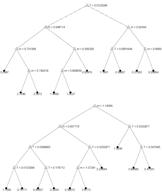
Regression tree (regtree) We fit a regression tree with 10 leaves to all ob-served IS call options and another regression tree with 10 leaves to all obob-served IS put options. Thus, the model depends on three location parameters (m, τ,cp flag) and 36 regression tree parameters (9 split variables and 9 cut values per regres-sion tree). Positivity of the IVS is guaranteed since the model depends on the aggregated observed positive IVs. See also Section4.1for further information.

3.3. MODELLING IVS DIRECTLY 35

Ad hoc BS model (adhocbs) Dumas et al.(1998) performed a goodness-of-fit

test for several functions of quadratic form in a deterministic volatility framework. They found that the best parametrization was given by

σ(K, τ) = max(0.01, a0+a1K+a2K2+a3τ +a4Kτ).

Since relative coordinates m = K/St and τ = T −t are used in this thesis, the model

σIV

ti =at0+at1mtiSt+at2(mtiSt)2+at3τti+at4mtiStτti+ǫti (3.16) is fitted by least square, using observations on day t. In case of negatively es-timated IV, values are also set to 0.01. The adhocbs model depends on (m, τ), factors ={St} and time-varying parameters at = (at0, at1, at2, at3, at4). The last

IS day ¯tis used as the reference day. Set a˜t=at¯to evaluate the IVS model on a future date ˜t >¯t.

Sticky moneyness model (stickym) The term ‘sticky moneyness’ denotes a broad class of ‘na¨ıve trader models’ (Cont and da Fonseca, 2002; Daglish et al., 2007). These models assume time invariance of the IVS for fixed moneyness. Such an assumption is only realistic for a short period and has to be understood in a ‘relative coordinate IVS random walk’ sense for OS predictions: the best guess for a point on the IVS of tomorrow at a fixed m location is a point on the IVS of today with the same m location. Further assumptions on the τ location are required to fully identify the point.

The stickym model is defined here in the following way: IS evaluation at any (m, τ) location is provided by data gridding. The focus of the used interpolation method15 is set to the geometrical aspect of the observed data {(mti, τti, σtiIV)|i=

15_{First, Delaunay triangulation is applied. The algorithm forms special triangles out of any}

given set of scattered data points in the (m, τ) plane such that the minimum angle of all trian-gles is maximized. Next, an estimate of the IVS is obtained via cubic interpolation over these triangles. Delaunay triangulation is important for computer graphics and finite element meth-ods to numerically solve PDEs. Watson (1992) is a reference for Delaunay triangulation-based applications in spatial data analysis.

36 CHAPTER 3. THE IMPLIED VOLATILITY SURFACE 1, ..., Lt}on dayt; the IVS is smooth, the monotonicity and the shape of the data are preserved. No extrapolation is conducted, and out-of-range values are set to the average IV on day t. The term structure of the IVS at the last IS day ¯t is used to interpolate the IV on a future date ˜t >¯t.

Bayesian vector autoregression (bvar) Doan, Litterman, and Sims(1984)

introduced a spatial econometric model that uses Bayesian prior information to overcome problems with high correlations in the data.

We implement the model as follows: First, a linearly spaced 10_×10 grid with values fromm = 0.2 to 2 and from τ = 1/365 to 3 is laid in the (m, τ) domain. For each IS day, IV is estimated on this grid using a Nadaraya-Watson estimator with a normal product kernel and stepwidth set according to the normal reference rule16.

Next, a Bayesian vector autoregression model of order 2 is fitted to this 100 dimensional time series of IV estimates on the fixed (m, τ) grid. A normal dis-tributed prior with mean 1 for coefficients associated with the lagged dependent variable in each equation of the vector autoregression and mean 0 for all other coefficients is imposed. In equation i of the vector autoregression, the standard deviation of the prior imposed on the dependent variablej at lagkis

sdijk = 0.2 w(i, j) k b sduj b sdui

where sdbui is the estimated standard error from a univariate autoregression in-volving variablei and W = [w(i, j)]_ij₌₁=1_,...,,...,₁₀₀100 is a matrix containing the values 1 fori=j. If the grid points corresponding to time series components iand j are neighbours,w(i, j) = 0.8 is set. All other entries ofW are set to 0.1. An internal grid point has at most eight neighbours. As a result of all these arrangements, only ca. 2% of the parameters are estimated significantly different from zero. LeSage (1999, p. 126) explains Bayesian vector autoregression models in the manual of

16_{Scott(1992) shows how to minimize the asymptotic integrated squared bias and asymptotic}

integrated variance for the multivariate normal product kernel. In the bivariate case, it is given by the sample standard deviation times number of observations to the power of−1/6.

3.3. MODELLING IVS DIRECTLY 37 his Econometrics Toolbox and provides functions to estimate, evaluate and fore-cast them. Between the fixed 100 grid points, we apply bicubic interpolation to evalutate the IVS at any (m, τ) location.

Dynamic semiparametric factor model (dsfm) Fengler, H¨ardle, and

Mam-men(2005;2007) describe dsfm as a type of functional coefficient model. “Surface estimation and dimension reduction is achieved in one single step. [The dsfm]can be seen as a combination of functional principal component analysis, nonparamet-ric curve estimation and backfitting for additive models” (2005, p. 6).

The dsfm model consists of smooth basis functions gk that are multiplied by time-varying latent factor loadings βt,k,

σIV_(m ti, τti) | {z } =σIV ti =g0(mti, τti)) + K X k=1 βt,kgk(mti, τti) +εmti,τti. (3.17)

The model is fitted to aggregated observed datat_∈IS=_{1, . . . , N_}, (mti, τti, σtiIV),

i∈ {1, ..., Lt} by minimizing a localized least square criterion.