Towards Robust Design and Training of Deep Neural Networks

(1)

TOWARDS ROBUST DESIGN AND TRAINING OF DEEP

NEURAL NETWORKS

An Undergraduate Research Scholars Thesis by

JEFFREY D. CORDERO

Submitted to the Undergraduate Research Scholars program at Texas A&M University

in partial fulfillment of the requirements for the designation as an

UNDERGRADUATE RESEARCH SCHOLAR

Approved by Research Advisor: Dr. Anxiao (Andrew) Jiang

May 2019

(2)

ABSTRACT

Towards Robust Design and Training of Deep Neural Networks

Jeffrey D. Cordero

Department of Computer Science and Engineering Texas A&M University

Research Advisor: Dr. Anxiao (Andrew) Jiang Department of Computer Science and Engineering

Texas A&M University

Currently neural networks run as software, which typically requires expensive GPU resources. As the adoption of deep learning continues for a more diverse range of appli-cations, direct hardware implemented neural networks (HNN) will provide deep learning solutions at far lower hardware requirements. However, Gaussian noise along hardware connections degrades model accuracy, an issue this research seeks to resolve using a novel analog error correcting code (ECC).

To aid in developing noise tolerant deep neural networks (DNN), this research also investigates the impact of loss functions on training. This involves alternating multiple loss functions throughout training, aiming to prevent local optimals. The effects on training time and final accuracy are then analyzed.

This research investigates analog ECCs and loss function variation to allow for future noise tolerant HNN networks. ECC results demonstrate three to five decibel improvements to model accuracy when correcting Gaussian noise. Loss variation results demonstrate a correlation between loss function similarity and training performance. Other correlations are also presented and addressed.

(5)

ACKNOWLEDGMENTS

"Surround yourself with the dreamers, and the doers, the believers, and thinkers, but most of all, surround yourself with those who see the greatness within you, even when you don’t see it yourself." -Edmund Lee [1]

Thanks primarily to my thesis advisor Dr. Anxiao Jiang, for allowing me freedom to guide my research while providing constant and valuable direction. You have been always available, understanding, and prepared to give meaningful guidance.

Thanks to the error correcting codes team, Yu Xiaojing, Palash Parmar, and Jacob Mink for your contributions to our publication, though primarily to Pulakesh Upadhyaya for allowing me a role in your fascinating research and for always being ready to provide significant answers.

To my father, Dr. Joehassin Cordero, for pushing me to achieve higher standards and improve, no matter how difficult; for wholly supporting my education, and for instilling both fascination and drive. You are truly my inspiration and my reason for success.

To my constant moral and emotional support, my mother Julie Cordero. Our daily conversations have been paramount to my growth. Thank you for being my cheerleader, no matter what.

To Dr. Luciano Castillo, for jump-starting my education through meaningful research involvement and challenging work experience before anyone else. I would not be pursing my dreams without your trust and investment in my life.

(6)

NOMENCLATURE

DNN Deep Neural Network

ECC Error Correcting Code

FER Facial Expression Recognition

HNN Hardware (Implemented) Neural Network

HP Hyperparameter

MSE Minimum Squared Error

NSR Noise-To-Signal Ratio

PDF Probability Density Function

(7)

LIST OF FIGURES

FIGURE Page

1.1 Basic neural network design [2] . . . 6

1.2 Local and Global minima, from [3] . . . 10

2.1 MNIST [4] sample data . . . 13

2.2 CIFAR10 [5] sample data . . . 13

3.1 FER2013 [6] sample data . . . 18

3.2 Classification visualizations for FER loss functions . . . 19

4.1 Theoretical verses observed minimum squared error. Note the two separate lines in each graph overlap. . . 24

4.2 Distortion experienced by the uncoded (noisy) weights verses that of the error corrected estimated weights . . . 25

4.3 The accuracy of estimated verses uncoded weights . . . 26

4.4 CIFAR10, Mean Squared Error (30) and Mean Squared Logarithmic Error (30), Using EarlyStopping . . . 28

4.5 CIFAR10, Categorical CrossEntropy(30) and Mean Squared Error (30), Using EarlyStopping . . . 29

4.6 CIFAR10, Categorical CrossEntropy(20), Mean Squared Error (20), and Hinge (20) . . . 30

4.7 FER, Mean Squared Error (30) and Mean Squared Logarithmic Error (30), Using EarlyStopping . . . 32

4.8 FER, Categorical Crossentropy (10) and Mean Squared Error (10), Using EarlyStopping . . . 33

(8)

LIST OF TABLES

TABLE Page

(9)

1. INTRODUCTION

Deep learning is a subfield of machine learning that implements algorithms inspired by the biological brain. These neural networks consist of multiple cascading layers of simple processing units, ‘neurons,’ with neurons connected to others in previous and following layers, as demonstrated by Figure 1.1. This layer-based design can learn data abstractions via supervised or unsupervised learning, proving invaluable for complex feature extraction tasks. For this reason, deep learning has quickly dominated the field of machine learning. It is often applied to problems like computer vision, natural language processing, and automatic image and text generation.

Figure 1.1: Basic neural network design [2]

1.1 Noise Correction in Hardware Neural Networks

Current deep learning solutions require powerful compute resources and complex soft-ware, adding vast overhead to working DNN solutions. Thus, the implementation of DNNs as dedicated hardware seeks to provide improved functionality at far reduced requirements.

(10)

1.1.1 Benefits of HNN networks

HNNs would reduce costs by lowering hardware requirements and decreasing power consumption. Reduced space would allow for further parallelism and distributed comput-ing, improving speed by orders of magnitude. Additionally, hardware implementations would benefit from graceful degradation, as hardware faults would reduce model perfor-mance. This is unlike software solutions which fail under system faults.[8] These benefits will allow deployment of DNN capabilities as embedded systems, providing deep learning solutions to environments and applications previously inaccessible to software versions.

1.1.2 Issues facing HNN networks

Although hardware implementations would provide many benefits over software so-lutions, they currently suffer performance loss from Gaussian noise. This noise impairs training by altering descent trajectory, increasing the cycles required for convergence, or making it outright impossible. Noise also degrades evaluation accuracy in trained models as its effects are propagated throughout the network, making high classification accuracy with large HNNs currently unobtainable. For this reason, HNNs are still a relatively small subfield of deep learning.

1.1.3 Simulating Noise

Modern computer hardware experiences Gaussian noise, noise with a probability den-sity function (PDF) equal to normal distribution. Simulating Gaussian [9] noise is accom-plished by generating uniform random samples before applying the Gaussian PDF

f(x) = (√ 1

2∗π)e

−x2

2 .

The quantity of noise affecting a system is measured using the signal-to-noise ratio (SNR), a measure of signal power, that is meaningful information, to background noise power,

(11)

unwanted interference [10]

SN R= Psignal

Pnoise often also expressed in decibels

SN Rdb = 10 log10

Psignal

Pnoise

.

The inverse of SNR is thus the systems noise-to-signal ratio (NSR)

N SR= 1

SN R.

To simulate hardware noise during experimentation, an additive white Gaussian noise channel alters all model weight with Gaussian noise of a given SNR.

1.1.4 Current Error Correction

To avoid noise induced message alteration, modern computing architecture implements binary signals for data representation. This provides natural fault tolerance as binary sig-nals are unaffected by minor signal variation. As well, binary communication can employ existing binary error correcting codes, including the famous 7, 4 Hamming Code [11], which adds redundancy via extra bits allowing receivers to detect and correct message errors without need for re-transmission.

Although HNNs do exist in use today, they currently only fit a small subset of appli-cations due to size and performance limits from noise perturbations. Examples include real-time embedded controllers [12], autonomous robotics [13], and character recognition [14].

(12)

1.2 Introduction to Loss Variation

Neural networks are typically trained using a single loss function, chosen by hyper-parameter tuning or personal experience. Loss variation describes a novel process of al-ternating multiple loss functions during network training. This research investigates the effects of training using loss variation, focused on training time and test accuracy. It also provides insight into how loss functions interact during training.

1.2.1 Introduction to Loss Functions

Loss functions provide a numeric evaluation of current network performance, quanti-fying the difference between expected output and actual model output. During training, the optimization algorithm continually works to minimize the loss value. The most common is gradient descent which computes the gradient of the loss function. Backpropagation ap-plies gradient descent to adjust neuron weights throughout the network. Although all loss functions have the same purpose, their numeric loss value depends on different equations. For this reason, some loss functions only apply to certain data types, for example cate-gorical verses binary outputs. Additionally, loss functions perform differently depending on model structure and hyperparameters, providing differing training times and evaluation accuracies.

1.2.2 Loss Variation Theory

In “A General and Adaptive Robust Loss Function” [15], Barron demonstrates im-proved model robustness and evaluation accuracy training with an automatically changing loss function based off L2 loss, generalized Charbonnier loss [16], and Welsch loss [17]. Otherwise, little research exists addressing switching loss functions as a training strategy.

Throughout training, loss function minimization leads to local ‘minima,’ where train-ing improvements level out. However, such local minima do not represent the most optimal

(13)

configuration, the global minima, as demonstrated in Figure 1.2. In theory, although loss functions have distinct local minima, their global minima should be similar, likely over-lapping. Therefore, switching loss functions would theoretically pull the model out of the previous function’s local minima, providing a better chance of reaching the global min-ima. If valid, this would substitute short term performance to improve resulting validation accuracy.

Figure 1.2: Local and Global minima, from [3]

1.2.3 Facial Expression Recognition

Facial expression recognition (FER), describes a challenging problem involving com-puter recognition of seven facial expression categories: anger, disgust, fear, happiness, sadness, surprise, and neutral. While facial expressions are a major part of human inter-action, their subtlety makes recognition difficult for computers, resulting in low validation accuracy. This low accuracy using traditional deep learning approaches makes FER a good

(14)

candidate for testing loss variation. 1.3 Objectives/Goals

This research investigates the intersection between these deep learning sub-fields to help develop noise tolerant DNN networks. This will aid in designing HNN architectures resistant to accuracy degradation from Gaussian noise. It first investigates a novel analog error correcting code to negate performance loss due to noise. It also determines whether training DNN networks using loss variation will increase performance.

(15)

2. ROBUST NEURAL NETWORKS WITH ERROR

CORRECTING CODES

The methodologies presented include the implementation and testing of an analog error correcting algorithm designed by Upadhyaya [18]. For each experiment, the measured value was plotted against decreasing SNR values and represents the average of twenty trials. Averaging was necessary due to the random nature of Gaussian noise, causing performance differences in each trial.

2.1 Network Architectures

Three smaller DNN models were identified that represent a range of purposes and network designs. This validates the developed ECC generalizes to the full range of modern DNN architectures and applications. Larger models were also tested, though presented separately [18].

Each model was implemented using the Keras [19] Python library with TensorFlow [20] backend. The models all came from the standard Keras library [19] as it represents a common source, eliminating additional variability. Each model was trained on its cor-responding dataset, ensuring high validation accuracy and preventing overfitting. After training, the neuron weights were saved to use the same weights for each experiment.

2.1.1 MNIST Model

The MNIST dataset [4] (Figure 2.1) contains 28x28 images of handwritten digits with 60,000 training and 10,000 testing images. The MNIST model is the smallest, with 1,199,882 weights in total. It is a convolutional network with two ReLU activated 3x3 convolutional layers that are fed into a 2x2 2D max pooling layer with 25% dropout, a flattening layer, a ReLU fully connected layer with 50% dropout, and finally a softmax

(16)

classifier.

Figure 2.1: MNIST [4] sample data

2.1.2 CIFAR-10 Model

The CIFAR-10 dataset [5] (Figure 2.2) consists of 32x32 color images falling into ten classes of 6,000 images apiece with 50,000 training and 10,000 testing images total. The CIFAR-10 model is a larger, convolutional network with 1,250,858 weights. It begins with four 3x3 ReLU activated convolutional layers split into two distinct blocks with each ending in 2x2 2D max pooling and 25% dropout layers. Finally, the network ends with a flattening layer feeding into a ReLU fully connected layer with 50% dropout and a softmax classifier.

(17)

2.1.3 IMDB Model

The IMDB dataset [7] (Table 2.1) contains 25,000 movie reviews prelabeled by senti-ment (positive/negative) from the IMDB website. As the data is textual, a recursive DNN network implementing long-short term memory (LSTM) modules was used for sequence processing. The model contains 2,691,713 weights total and begins with an embedding layer from 20,000 to 128. This is fed into size 128 LSTM modules with 20% dropout and 20% recurrent dropout. The model terminates with a sigmoid activated fully connected layer of size one since classifying binary sentiment.

Table 2.1: IMDB [7] sample data

Positive I liked this movie a lot. It really intrigued me how Deanna and Alicia became friends over such a tragedy. Alicia was just a troubled soul and Deanna was so happy just to see someone after being shot.

Negative This movie was messed up. A sequel to “John Carpenter’s Vampires,” this didn’t add up right. I’m not sure that I enjoyed this much.

2.2 Measuring Performance Degradation From Noise

The following steps represent the major development stages for assuring valid ECC implementation and obtaining experimental results. The first step studied DNN network performance with weights perturbed by Gaussian noise of increasing variance. This pro-vided a performance baseline for expected accuracy of hardware based models not using any error correction techniques. For each variance, calculated from corresponding SNRs, the weights were altered by adding values from a Gaussian normal distribution before re-evaluating the model’s validation accuracy.

Starting off, mean µ and variance Du of all weights was calculated. The weights were then divided into K×1 sized vectors (K = 30 for all experiments presented), each represented by w. Next,w was converted into its corresponding zero mean equivalent u

(18)

by subtractingµ, such that for eachwi,

ui =wi−µ

The zero mean weightsuwere then encoded to corresponding codeword vectors using the generator matrix G. This K×N matrix was used to encode each K weight vector into its N size codeword vector, where N>K. TheGmatrix ensures the energy per information bit is Eb, thus being scaled by a factor of

q Eb

Du. (N-K) rows were then deleted from the originally orthogonal matrix. Therefore, the final G satisfies

GGT =diag{Eb Du , Eb Du , ..., Eb Du }

The generator matrix is used to obtain N size codeword vectorsvfromu. Each includes redundant information, the N-K excess symbols, allowing for approximating the original values after perturbation from noise.

v =GTu

The variance of all codeword values was then calculated and used as the energy per information bitEb when solving for the standard deviation of Gaussian noiseσ. That is, solving SN R = 10 log₁₀(Eb σ2) using σ = s Eb 10SN R10

To simulate an additive white Gaussian noise channel, Gaussian noisenwas generated by selecting random normal values between 0 andσ. This noise was added to obtain noisy

(19)

codeword vectorsrusing

r=v+n

before selected the first K elements of each codeword vector and re-adding the original meanµ

unoisy =rf irstK+µ

This simulated hardware based noise perturbation like that of a more complex system implementing error correction methods.

2.3 Applying Error Correction

The second step involved applying an analog ECC to estimate the original weights from noise altered codeword vectors. After following the method from step one to gen-erate codeword vectors, and adding noise to simulate physical message transmission, the codeword was decoded touˆ, the estimated values of the originaluweight values.

ˆ

u=Ar

for decoder matrix

A= (GGT)−1G

Finally, the noise corrected, estimated weight valueswˆwere recovered by re-addingµ.

ˆ

wi = ˆui +µ

2.4 Comparing Theoretical and Experimental Performance

The third stage involved comparing theoretical and experimental error correction per-formance to ensure correct implementation. Although experimental perper-formance cannot

(20)

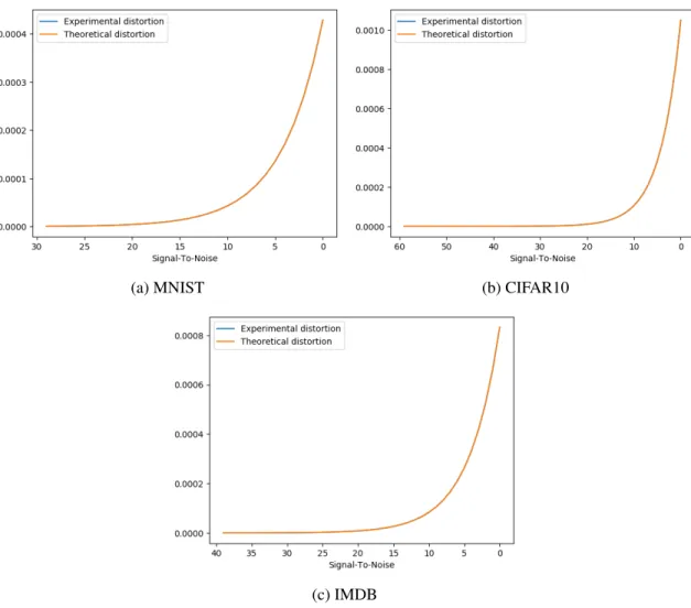
achieve theoretical performance, being close implies correct ECC implementation. The experimental minimum squared error (MSE), that is experimental distortion, was obtained and plotted alongside the calculated theoretical distortion as demonstrated in Figure 4.1.

The sample MSE was computed for each K-size weight vectorwiand its corresponding estimated weight vectorwˆi,

∆sample M SE = 1 K K X i=1 (wi−wˆi)2

The experimental MSE was then calculated using all sample errors

∆exper M SE = 1 num_samples X num_samples ∆sample M SE

Finally the experimental MSE is compared to the theoretical MSE as calculated using maximum likelihood:

∆M L= Duσ

2

Eb

2.5 Evaluating Model Accuracy With Corrected Weights

To observe accuracy improvements from the ECC, model test set accuracy was evalu-ated first with the noisy, uncorrected weights,unoisy, then with the estimated weights,wˆi, obtained by the decoding phase. This entire process, including adding noise and applying the ECC, was run 30 times for each SNR value. The results were then averaged, producing the best performance estimation for the given noise quantity. Averaging was necessary due to Gaussian noise’s inherent randomness, causing differing amounts of noise throughout the model, leading to a wide range of evaluation accuracies. These averaged accuracies were then plotted to produce Figure 4.3.

(21)

3. LOSS VARIATION METHODOLOGY FOR ROBUST

TRAINING

A challenging problem in deep learning, facial expression recognition (FER) was se-lected to test the training capabilities of loss variation. This involved developing a model for the FER2013 dataset and experimentation with specialty FER loss functions. Training with loss variation was then carried out on a range of models and sets of loss functions. Loss interaction experiments then investigated how loss functions interact as part of loss variation.

3.1 FER2013 Dataset

FER2013 [6] (Figure 3.1) is a challenging dataset containing 48x48 size grey scale images of seven facial expression classifications, angry (4,593 images), disgust (547), fear (5,121), happy (8,989), sad (6,077), surprise (4,002), and neural (6,198). In total, it provides 28,709 training, 3,589 validation, and 3,589 test images.

Figure 3.1: FER2013 [6] sample data

3.2 FER Network Architecture

The model developed for the FER2013 dataset is a convolutional network containing 1,485,831 weights total. It begins with a 5x5 ReLU activated convolutional layer fed into 2x2 2D max pooling. This leads to two convolutional blocks, each containing two 3x3 ReLU convolutional layers and a 2x2 2D average pooling layer. The model then applies

(22)

a flattening layer fed into two ReLU 1024 size fully connected layers with 20% dropout each. The output is then split, the first being a size 10 softmax activated dense layer for use with standard loss functions (namely softmax). The second is a size 2 ReLU dense layer providing input (x, y) positions and representing their classification relative to class centers. This special output is fed through custom FER loss functions, center loss and island loss.

3.3 Custom FER Loss Functions

Although FER models can and do use standard loss functions for training, specialty ones improve training performance by increasing classification distance between class cen-ters and decreasing inter-set distance around cencen-ters. The loss functions described below are visualized in Figure 3.2.

(a) Softmax loss + center loss (b) Softmax loss + island loss (c) Softmax + center + island

Figure 3.2: Classification visualizations for FER loss functions

3.3.1 Softmax Loss

The softmax function is applied to the standard model output in FER networks. How-ever, softmax is not actually a loss function, it is an activation function that provides clas-sification probabilities for class based loss functions, typically cross-entropy loss. These classification probabilities are normalized to sum to one. For each samplezi, for all

(23)

possi-ble classifications {1,...,K}:

σ(z)j =

ezj PK

k=1ezj

Cross-entropy loss then provides a loss value using the classification probabilities ob-tained by softmax. For each iterationi, using true labelsy, and model predictionsyˆ:

H(p, q) =−X

i

pilogqi =−ylog ˆy−(1−y) log(1−yˆ)

3.3.2 Center Loss

Center Loss [21] improves classification by penalizing the distance between features and their corresponding class centers, therefore reducing intra-class variation. For the ith

sample, having class labelyi and feature vectorxi, andCyi ∈ IRd being the center of all samples with the same class label:

LCL= 1 2 m X i=1 xi−Cyi 2 2 3.3.3 Island Loss

Island loss [22] improves classification by increasing the pairwise distance between different class centers. For the set ofN expression labels, whereCkandCj are thekthand

jth _{cluster centers:} LIL = X Cj∈N X Ck∈N,Ck∈/Cj Ck·Cj kCkk2 C_j 2 + 1 !

3.3.4 Experimental Loss Function

To alternate center and island loss loss variation experimentation, the loss function used was a summation of each function with a corresponding hyperparameterαLoss, set to

(24)

0 when not in use:

L=αSLS+αCLLCL+αILLIL

During training, cluster centers were updated by subtracting the center update ∆Ct j, scaled by hyperparameterα, from current positionCt

j:

C_jt+1 =C_jt−α∆C_jt

The center update∆C_jtis computed as follows, whereδ(yi, i)represents whether the given sampleyiis in setj:

∆Cj = Pm i=1δ(yi, j)(Cj −xi) 1 +Pm_i₌₁δ(yi, j) δ(yi, i) = ( 0 if yi =j 1 if yi 6=j 3.4 Experimental Process for Loss Variation

This research required extensive experimentation to understand loss function interac-tions during training. Therefore, an automated test suite was developed for efficient testing with many different models and various sets of loss functions. Starting with the first loss function, the model was trained to a local minima, applying early stopping to identify when achieved. The stage’s training history was then recorded before re-starting training with the next loss function. After all loss functions have been used, it begins again with the first. Training was concluded when the loss values begin ‘oscillating,’ where the differ-ence in a given loss function’s validation loss after each training cycle was within a given range.

(25)

3.5 Experimental Process for Loss Interaction

As observable by the loss variation results (section 4.2), loss functions seem to inter-act negatively. Because of this, additional experimentation analyzed whether loss values were optimal when training with their corresponding loss function. This sought to pro-vide insight into how loss functions interact. If a loss value was always lowest for its loss function, this would demonstrate they indeed optimize the model against each other.

Testing was straightforward, the model was trained to completion with each loss func-tion. During training, the value of every loss function was evaluated on the entire training set after each epoch. By comparing the resulting loss values, it would then be demonstrated whether loss functions interact negatively.

(26)

4. EXPERIMENTAL PERFORMANCE AND ANALYSIS

This chapter begins with results pertaining to noise reduction in analog ECCs. It begins by ensuring correct ECC implementation before presenting accuracy-based performance results. Loss variation experiments are then presented, specifically those tests which best present observed correlations. Finally, results for testing loss function interactions are given.

4.1 Experimental Performance for Robust Neural Networks With Error Correcting Codes

Correct ECC implementation is demonstrated by comparing theoretical and experi-mental minimum squared error (MSE) as well as observing distortion reduction between uncoded and experimental distortion. ECC Performance is then presented comparing model accuracy when evaluated with ECC estimated weights and uncoded weights.

4.1.1 Minimum Squared Error

Minimal difference between theoretical and experimental MSE implies a valid ECC implementation. Even functioning optimally, ECCs cannot achieve perfect estimations after perturbations from noise. Therefore, as long as the experimental MSE distortion from the estimated weights approaches theoretical distortion, the ECC has been correctly implemented and the accuracy results will be valid.

Although it appears only theoretical performance is plotted in Figure 4.1, this is ac-tually not the case. For all three models, the experimental and theoretical performance are equal to a precision unable to be observed here. This allows confidence the accuracy results will be correct.

(27)

(a) MNIST (b) CIFAR10

(c) IMDB

Figure 4.1: Theoretical verses observed minimum squared error. Note the two separate lines in each graph overlap.

4.1.2 Uncoded Verses Experimental Distortion

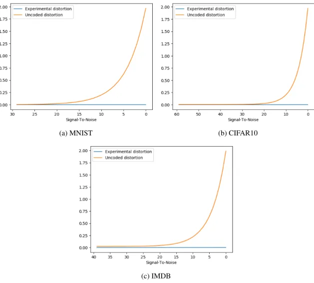
As SNR decreases, noise increases in relation to signal strength, thus causing more distortion in the system. While the ECC seeks to negate this fault, its estimations can never perfectly reduce such errors. However, by comparing the amount of distortion experienced by the uncoded, noisy weights and the experimental, estimated weights, we can observe the ECC’s ability to reduce such distortion.

Although it appears in Figure 4.2 that the experimental results contain no distortion, this is not true. The experimental results in 4.2 are the same as those in Figure 4.1, but

(28)

when plotted against the uncoded results, it demonstrates how well the ECC performs.

(c) IMDB

Figure 4.2: Distortion experienced by the uncoded (noisy) weights verses that of the error corrected estimated weights

4.1.3 Observed Accuracy

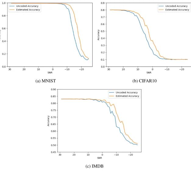
Naturally a hardware implemented DNN would only be viable if test set accuracy approached that of its original, software based counterpart. Such accuracy results are pre-sented in Figure 4.3, comparing accuracy with both ECC estimated weights and uncoded weights. It should be noted that the plots are of different scales due to initial model accu-racy and number of data set classes. MNIST and CIFAR-10 drop to 10% accuaccu-racy at low

(29)

SNRs since there exists a one in ten chance of random chance success. IMDB only has two possible classifications on the other hand.

As observable by the estimated accuracy lines, the models all display a natural tol-erance to lower quantities of noise (higher SNR values). This toltol-erance varies however, as the SNR value where a model’s performance begins to drop-off differs significantly. Drop-off then occurs relatively quickly for all models, descending to random chance over a small SNR interval.

(c) IMDB

(30)

Of course significant performance differences between models is to be expected and yet quite insightful. Previous research [18] demonstrated that noise introduced in earlier model layers causes more significant performance degradation. Therefore, larger models should experience greater accuracy loss as noise perturbations at initial model layers are exacerbated though more layers. It may also be the case that the increased dropout per-centages of MNIST and IMDB are improving the model’s resilience to noise, similar to adding Gaussian noise during training to prevent overfitting as presented by [23].

When comparing the estimated and uncoded accuracy lines in Figure 4.3, the perfor-mance improvement from the ECC can be seen as it right-shifts the drop-off to lower SNR values. By comparing similar accuracies between the two lines and subtracting their corre-sponding SNR values, this right-shifting can be found to improve accuracy between three and five decibels for all models.

4.2 Experimental Performance for Training With Loss Variation

Due to differences in model design and dataset complexity, loss variation experiments were run on both CIFAR-10 and FER models. Note in the following graphs, dotted lines imply swapping loss functions and near vertical changes in loss value are caused by dif-ferent loss functions which scale their loss values difdif-ferently.

4.2.1 CIFAR10 Model Results

As presented below, CIFAR-10 results demonstrate complex interactions between loss functions affecting training success. Results suggest that alternating training with more similar loss functions provides more stable training, but may also suffer overfitting. On the other hand, very different loss functions seem to quickly degrade model performance, inducing wide oscillations in model loss and harming accuracy.

(31)

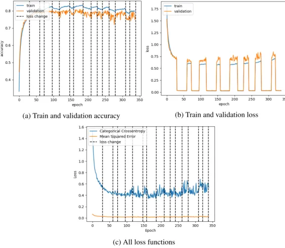
4.2.1.1 Mean Squared Error And Mean Squared Logarithmic Error

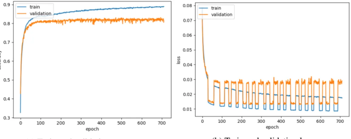
Demonstrated by Figure 4.4, the similar loss functions seem to train the model like a single loss function, providing smooth loss decline. However, the training accuracy increases while keeping validation accuracy constant, appearing to prevent overfitting from decreasing validation performance.

(a) Train and validation accuracy (b) Train and validation loss

(c) All loss functions

Figure 4.4: CIFAR10, Mean Squared Error (30) and Mean Squared Logarithmic Error (30), Using EarlyStopping

4.2.1.2 Categorical Crossentropy And Mean Squared Error

In Figure 4.5, loss function differences appear to introduce mild disturbances, increas-ing loss and accuracy instability over loss change cycles. Additionally, while both loss

(32)

functions typically perform well for CIFAR-10, the training accuracy increases during mean squared error but decreases during categorical crossentropy. Although validation loss is not degraded too heavily, training loss is kept far lower than usual.

Figure 4.5: CIFAR10, Categorical CrossEntropy(30) and Mean Squared Error (30), Using EarlyStopping

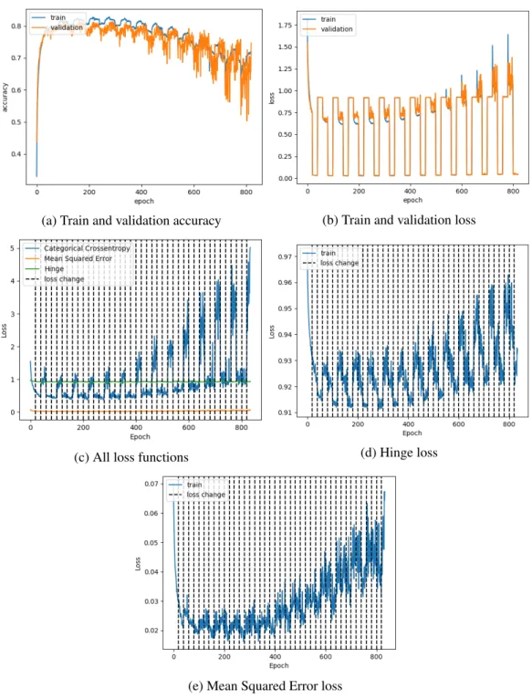
4.2.1.3 Categorical Crossentropy, Mean Squared Error, and Hinge

Figure 4.6 represents the worst performance observed from this training technique. It involved training with three loss functions that are functionally quite different and for more cycles than other tests. Throughout training, both training and validation accuracy drop at an increasing rate. Additionally, validation accuracy becomes extremely unstable,

(33)

oscillating until it manages to surpass training accuracy at some points. Notice in 4.6c, 4.6d, and 4.6e, that different loss functions’ values oscillate wildly thoughout training, highest when the model is being trained with a different loss function.

(c) All loss functions (d) Hinge loss

(e) Mean Squared Error loss

(34)

4.2.2 Facial Expression Recognition Model Results

The FER model demonstrated a behavior unseen in CIFAR-10, whereas switching the loss function causes a sudden drop in training accuracy and spike in each loss function’s loss value. As the loss value of each independent loss function was evaluated on the entire training set separately of the training process, it can be confirmed that swapping loss functions somehow affects the model directly. This prompted further research into how loss functions interact with each other, presented in 4.2.3.

4.2.2.1 Mean Squared Error and Mean Squared Logarithmic Error

Similar to the CIFAR-10 version (Figure 4.4), Figure 4.7 presents stable training when cycling similar loss functions.

(35)

Figure 4.7: FER, Mean Squared Error (30) and Mean Squared Logarithmic Error (30), Using EarlyStopping

4.2.2.2 Categorical Crossentropy and Mean Squared Error

Unlike the CIFAR-10 version (Figure 4.5), Figure 4.8 does not demonstrate oscilla-tions in accuracy. Instead, validation accuracy remains smooth, increasing slowly over time. Training accuracy and training loss also remain smooth, besides initial spikes after switching loss functions.

(36)

(c) Categorical Crossentropy loss (d) Mean Squared Error loss

Figure 4.8: FER, Categorical Crossentropy (10) and Mean Squared Error (10), Using EarlyStop-ping

4.2.3 Loss Interactions

Experiments on loss function interactions measured all loss values while training to completion with a single function. This presented negative results of any correlation be-tween training function and minimization of its loss value. Instead, for each model a single loss function provided the highest validation accuracy and the lowest loss values for all loss functions. This implies that training issues from loss switching are not caused by loss functions optimizing the model in some specific manner.

(37)

5. CONCLUSIONS AND FUTURE WORK

This research investigated two approaches that could enable noise tolerant HNNs in the future. A novel ECC demonstrated three to five decibel accuracy improvements when correcting weights perturbed by Gaussian noise. Loss Variation then presented a new training approach that could improve model performance.

5.1 Concluding Remarks and Future Work on Robust Neural Networks

Although previous research existed on introducing Gaussian noise to improve DNN training, [23] none has investigated how noise effects evaluation performance. This re-search has demonstrated DNNs have some natural tolerance to Gaussian noise, with greater tolerance corresponding to smaller networks. Additionally, although performance drop-off begins at differing SNR values, complete accuracy loss occurs over a small SNR range, following a similar pattern for all networks.

This research also presented a novel analog ECC able to estimate decimal point val-ues altered by additive white Gaussian noise. It then demonstrated the ECC’s ability to improve accuracy in simulated hardware implemented DNNs. Such a solution could aid in future development of dedicated neural network hardware using analog signals for effi-ciency.

5.1.1 Further Research

Being a new topic in deep learning, there is plenty of future research available, includ-ing implementation into physical hardware. However, most should involve the develop-ment of more efficient error correction techniques. Although increased redundancy would improve code estimations, this adds overhead to the encoding and decoding processes and increases the amount of information required to be transmitted. Therefore, future research

(38)

should investigate the optimal amount of redundancy, providing the best trade-off between improved estimations and performance overhead.

This research also leaves open the possibility of different forms of analog ECCs. Pre-vious research proved noise introduced in earlier network layers decreases accuracy more than later layers [18]. Therefore, a code prioritizing greater amounts of redundancy for earlier layers could improve model performance while maintaining less overhead.

5.2 Concluding Remarks and Future Work on Robust Training

Training using multiple loss functions presented complex but interesting interactions. Experiments with CIFAR-10 demonstrated a correlation between loss function similarity and training performance. As increasingly distinct loss functions were used, oscillation increased and training performance decreased. This also seemed true of more loss func-tions. However, such observations appear less true of the FER model, where loss would spike and accuracy drop immediately after swapping loss functions. Yet after only a few training epochs both would return to previous or better performance. This need to recover from initial spikes may be the reason FER demonstrated less oscillations from less similar loss functions. If so, such an approach may be applicable when training models on difficult datasets.

5.2.1 Further Research

Going forward, experimentation with more datasets and models could provide further correlations between dataset difficulty, model size, and loss variation success. Continued experimentation with different loss function sets could verify that decreased loss function similarity leads to decreased accuracy and greater loss value oscillation. Investigating the reason behind loss spikes after loss function swapping in the FER model could also prove insightful. This is possibly caused by the complexity and difficulty of the FER2013 dataset and testing loss variation on other difficult datasets could demonstrate whether this

(39)

is correct. It may also be possible to reduce spikes by increasing model size to reduce sensitivity. Overall, experimentation investigating why loss functions interact negatively could provide better insight into how deep learning models train.

(40)

REFERENCES

[1] A. Meah, “30 quotes on positive associations to inspire you to surround yourself with the best,” Dec 2016.

[2] Ž. Ivezi´c, A. Connolly, J. Vanderplas, and A. Gray, Statistics, Data Mining and Machine Learning in Astronomy. Princeton University Press, 2014.

[3] A. Kathuria,Local and Global Minima. Jun 2018.

[4] Y. LeCun, L. Bottou, Y. Bengio, and P. Haffner, “Gradient-based learning applied to document recognition,” inProceedings of the IEEE, vol. 86, pp. 2278–2324, 1998.

[5] A. Krizhevsky, “Learning multiple layers of features from tiny images,” University of Toronto, 05 2012.

[6] I. Goodfellowet al., “Challenges in representation learning: A report on three ma-chine learning contests,” 2013.

[7] A. L. Maas, R. E. Daly, P. T. Pham, D. Huang, A. Y. Ng, and C. Potts, “Learning word vectors for sentiment analysis,” in Proceedings of the 49th Annual Meeting of the Association for Computational Linguistics: Human Language Technologies, (Portland, Oregon, USA), pp. 142–150, Association for Computational Linguistics, June 2011.

[8] J. Misra and I. Saha, “Artificial neural networks in hardware: a survey of two decades of progress,”Neurocomputing, vol. 74, no. 1, pp. 239 – 255, 2010. Artificial Brains.

(41)

[9] D. U. Lee, W. Luk, J. D. Villasenor, and P. Y. Cheung, “A gaussian noise generator for hardware-based simulations,”IEEE Transactions on Computers, vol. 53, no. 12, pp. 1523–1534, 2004.

[10] R. Kieser, P. Reynisson, and T. J. Mulligan, “Definition of signal-to-noise ratio and its critical role in split-beam measurements,”ICES Journal of Marine Science, vol. 62, no. 1, pp. 123–130, 2005.

[11] Z. Li, S.-J. Lin, and H. Hu, “On the arithmetic complexities of hamming codes and hadamard codes,” vol. 14, no. 8, pp. 1–22, 2018.

[12] L. M. Reyneri, M. Chiaberge, and L. Zocca, “CINTIA: A neuro-fuzzy real time con-troller for low power embedded systems,” Proceedings of the Fourth International Conference on Microelectronics for Neural Networks and Fuzzy Systems, pp. 392– 403, 1994.

[13] S. Bellis et al., “Fpga implementation of spiking neural networks - an initial step towards building tangible collaborative autonomous agents,” Proceedings. 2004 IEEE International Conference on Field-Programmable Technology (IEEE Cat. No.04EX921), 2004.

[14] D. Kim, H. Kim, G. Han, and D. Chung, “A SIMD neural network processor for image processing,”Advances in Neural Networks, 2005, vol. 3497, p. 815, 2005.

[15] J. T. Barron, “A more general robust loss function,” CoRR, vol. abs/1701.03077, 2017.

[16] D. Sun, S. Roth, and M. Black, “Secrets of optical flow estimation and their princi-ples,” vol. 1, pp. 2432–2439, Sept 2010.

(42)

[17] J. E. D. Jr. and R. E. Welsch, “Techniques for nonlinear least squares and robust re-gression,”Communications in Statistics - Simulation and Computation, vol. 7, no. 4, pp. 345–359, 1978.

[18] P. Upadhyaya, X. Yu, J. Mink, J. Cordero, P. Parmar, and A. Jiang, “Error correction for noisy neural networks,” in2019 Information Theory and Applications Workshop.

[19] F. Cholletet al., “Keras.”https://keras.io, 2015.

[20] M. Abadiet al., “TensorFlow: Large-scale machine learning on heterogeneous sys-tems.”www.tensorflow.org, 2015.

[21] Y. Wen, K. Zhang, Z. Li, and Y. Qiao, “A discriminative feature learning approach for deep face recognition,” inECCV, 2016.

[22] J. Cai, Z. Meng, A. S. Khan, Z. Li, J. OReilly, and Y. Tong, “Island loss for learning discriminative features in facial expression recognition,” pp. 302–309, May 2018.

[23] Y. Li, R. Xu, and F. Liu, “Whiteout: Gaussian adaptive regularization noise in deep neural networks,” Dec 2016.