On the spatial modelling of mixed and constrained geospatial data

(1)

Edith

Cowan

University

Copyright

Warning

You

may

print

or

download

ONE

copy

of

this

document

for

the

purpose

of

your

own

research

or

study.

The

University

does

not

authorize

you

to

copy,

communicate

or

otherwise

make

available

electronically

to

any

other

person

any

copyright

material

contained

on

this

site.

You

are

reminded

of

the

following:



Copyright

owners

are

entitled

to

take

legal

action

against

persons

who

infringe

their

copyright.



A

reproduction

of

material

that

is

protected

by

copyright

may

be

a

copyright

infringement.

Where

the

reproduction

of

such

material

is

done

without

attribution

of

authorship,

with

false

attribution

of

authorship

or

the

authorship

is

treated

in

a

derogatory

manner,

this

may

be

a

breach

of

the

author’s

moral

rights

contained

in

Part

IX

of

the

Copyright

Act

1968

(Cth).



Courts

have

the

power

to

impose

a

wide

range

of

civil

and

criminal

sanctions

for

infringement

of

copyright,

infringement

of

moral

rights

and

other

offences

under

the

Copyright

Act

1968

(Cth).

Higher

penalties

may

apply,

and

higher

damages

may

be

awarded,

for

offences

and

infringements

involving

the

conversion

of

material

(2)

On the spatial modelling of mixed and

constrained geospatial data

by

Hassan Talebi

(MESc)

A Thesis with Publications presented to Edith Cowan University in fulfilment of the requirement for the degree of

Doctor of Philosophy

School of Science Edith Cowan University Joondalup, WA 6027, Australia

2018

(3)

ii

Abstract

Spatial uncertainty modelling and prediction of a set of regionalized dependent variables from various sample spaces (e.g. continuous and categorical) is a common challenge for geoscience modellers and many geoscience applications such as evaluation of mineral resources, characterization of oil reservoirs or hydrology of groundwater. To consider the complex statistical and spatial relationships, categorical data such as rock types, soil types, alteration units, and continental crustal blocks should be modelled jointly with other continuous attributes (e.g. porosity, permeability, seismic velocity, mineral and geochemical compositions or pollutant concentration). These multivariate geospatial data normally have complex statistical and spatial relationships which should be honoured in the predicted models.

Continuous variables in the form of percentages, proportions, frequencies, and concentrations are compositional which means they are non-negative values representing some parts of a whole. Such data carry just relative information and the constant sum constraint forces at least one covariance to be negative and induces spurious statistical and spatial correlations. As a result, classical (geo)statistical techniques should not be implemented on the original compositional data. Several geostatistical techniques have been developed recently for the spatial modelling of compositional data. However, few of these consider the joint statistical and/or spatial relationships of regionalized compositional data with the other dependent categorical information.

This PhD thesis explores and introduces approaches to spatial modelling of regionalized compositional and categorical data. The first proposed approach is in the multiple-point geostatistics framework, where the direct sampling algorithm is developed for joint simulation of compositional and categorical data. The second proposed method is based on two-point geostatistics and is useful for the situation where a large and representative training image is not available or difficult to build. Approaches to geostatistical simulation of regionalized compositions consisting of several populations are explored and investigated. The multi-population characteristic is usually related to a dependent categorical variable (e.g. rock type, soil type, and land use). Finally, a hybrid predictive model based on the advanced

(4)

iii

geostatistical simulation techniques for compositional data and machine learning is introduced. Such a hybrid model has the ability to rank and select features internally, which is useful for geoscience process discovery analysis.

The proposed techniques were evaluated via several case studies and results supported their usefulness and applicability.

Keywords: compositional data, two-point geostatistics, multiple-point geostatistics, machine leaning, spatial predictive models.

(5)

iv

Declaration

I certify that this thesis does not, to the best of my knowledge and belief:

i. Incorporate without acknowledgement any material previously submitted for a degree or diploma in any institution of higher education;

ii. Contain any material previously published or written by another person except where due reference is made in the text;

iii. Contain any defamatory material.

I also grant permission for the Library at Edith Cowan University to make duplicate copies of my thesis as required.

Signed: Hassan Taleb

(6)

v

Acknowledgements

I wish to express my sincere gratitude to those people without whom it would not be possible for me to undertake this program during my years at Edith Cowan University.

I sincerely thank my Principal Supervisor, Associate Professor Ute Mueller, and Associate Supervisor, Dr. Johnny Lo, for their invaluable time, continuous moral support, insightful guidance and constructive criticism since the start of the program. I would like to acknowledge Dr Raimon Tolosana-Delgado and Professor Karl Gerald van den Boogaart for their contribution to the development of proposed algorithms and implementations.

I am thankful to the technical and administrative staff of the School of Science at ECU for their assistance with regard to the project. The PhD research project was made possible by an Edith Cowan University International Postgraduate Research Scholarship (ECU-IPRS).

The anonymous reviewers of different internationally recognized journals and the thesis are also thanked for their precious time and scholarly comments which were helpful in further developing the manuscripts.

(7)

vi

List of Journal Publications Arising from this Candidature

Published Book Chapter

 Talebi H, Lo J, and Mueller U (2017). A hybrid model for joint simulation of high-dimensional continuous and categorical variables. In: J.J. Gómez-Hernández, J. Rodrigo-Ilarri, M.E. Rodrigo-Clavero, E. Cassiraga and J.A.

Vargas-Guzmán (Editors), Geostatistics Valencia 2016. Springer

International Publishing, Cham, pp. 415-430.

Accepted Journal Paper

 Talebi H, Mueller U, Tolosana-Delgado R, van den Boogaart K G (2018).

Geostatistical simulation of geochemical compositions in the presence of multiple geological units - Application to mineral resource evaluation.

Mathematical Geosciences, DOI: 10.1007/s11004-018-9763-9.

Journal Papers Under Review

 Talebi H, Mueller U, Tolosana-Delgado R, (2018). Joint simulation of compositional and categorical data via direct sampling technique - Application to improve mineral resource confidence. Computer & Geosciences, Under Review.

 Talebi H, Mueller U, Tolosana-Delgado R, Grunsky, E C, McKinley J M,

Caritat P de (2018). Surficial and deep earth material prediction from geochemical compositions, a spatial predictive model, Natural Resources Research, Under Review.

(8)

vii

List of Figures

Figure 2-1 The variation of bias (systematic over or underestimation) for the simulated model across several cut-offs on the three variables of interest ... 31 Figure 2-2 Locations of input data (a) and simulation nodes (b) in the study area32 Figure 2-3 2D synthetic case study, a) locations of input data and simulation nodes, b) spatial patterns of three geological domains, c) and d) value component #1 and #3, e) deleterious component #2, f) filler component #4 ... 33 Figure 2-4 Stacked histogram of the four components of input and validation sets, coloured by the proportion of domains in each bin ... 34

Figure 2-5 Ternary diagrams of the sub-compositions for input and validation sets, coloured by domains (small triangles) and kernel density (large triangles) ... 34 Figure 2-6 Histogram reproduction for the three zones. Continuous and dotted lines (dark colours) are input and validation data respectively, while lines with light colours are simulations ... 36 Figure 2-7 Ternary diagrams (three components of interest) of the input data, validation data, and one randomly selected realization for the three simulation zones ... 38 Figure 2-8 Reproduction of experimental variogram in the three simulation zones (continuous black lines are input data, dashed black lines are validation data, and grey lines are realizations) ... 39 Figure 2-9 Spatial distribution of domains and compositions. First column is the validation set, second column is one randomly selected realization and the last column is the expected model ... 40 Figure 2-10 Top: total compositional variation calculated from realizations (warm colours show high values while cold colours show low values) and true doamins from validation set (bottom) ... 41 Figure 2-11 Difference between the expected proportions above various cut-offs on three components of interest (component #1 to #3), calculated from realizations, and real proportions calculated from the validation data ... 44

(13)

xii

Figure 2-12 Perspective view of the Murrin Murrin data. a) locations of input data and simulation nodes. b) spatial distribution of the four geological units. c) to h) six components of interest in the form of composition ... 46 Figure 2-13 Histogram of the geochemical components (input and validation sets), coloured by the proportion of rock types in each bin ... 47 Figure 2-14 Ternary diagrams of the centred geochemical compositions of input and validation sets, coloured by rock types (small triangles) and kernel density (large triangles). ... 47

Figure 2-15 Histogram reproduction of the five components of interest in the four geological units. Continuous and dotted lines (dark colours) are input and validation data respectively, while lines with light colours are simulations ... 50 Figure 2-16 Ternary diagrams of a sub-composition (Ni-Co-Fe) of input data, validation data, and one randomly selected simulation, coloured by the rock types (second row) and kernel density (first row) ... 50 Figure 2-17 Contact analysis of total compositional variation for the geological units ... 51 Figure 2-18 Grade-tonnage curves (for Ni and Co component) of the four geological units. Continuous black lines are the proportions of samples above cut-off for the input data, while dashed black lines are computed from the validation data. Continuous red lines are the average grades above cut-offs for the input data, while red dashed lines are computed from the validation data. Grey lines are different realizations ... 52 Figure 2-19 Difference between the expected proportions above the cut-offs of four components of interest (Ni, Co, Fe, and Mg), calculated from realizations, and real proportions calculated from the validation data ... 53 Figure 3-1 Process of the joint simulation technique. ... 62

Figure 3-2 Perspective view of samples showing a) different rock types and b) Nickel grade. ... 63

Figure 3-3 Rock types (colored data), nickel (left), and cobalt (right) distributions for the cross-section with north coordinate 180 m. ... 64

(14)

xiii

Figure 3-4 Histograms of raw data. ... 64 Figure 3-5 Truncation rule indicating relationship between four rock types. ... 66 Figure 3-6 Experimental variograms and fitted model for the first factor. ... 69 Figure 3-7 Perspective view of a) one realization of Ni grade, b) mean of the simulated Ni grade, c) one realization of rock types and d) most probable simulated rock type. ... 72 Figure 3-8. Q-Q plots of realizations of the major elements against sample data. 73 Figure 3-9 Boxplot of realisation proportions for the four rock types – the sample proportions are indicated by a black horizontal line, the exhaustive proportions by a red horizontal line. ... 73 Figure 3-10 Experimental cross-variograms between rock type indicators and Ni grade, for sample data (black line) and simulated realizations (dashed line). ... 74 Figure 3-11 a) Contact analysis between FZ and SA domains for sample Ni grade (black graph), mean of simulated Ni grade (continuous red graph), and a realization of Ni grade (dashed red graph). b) Average prediction error for Ni grade compared with exhaustive data set. ... 74 Figure 4-1 Geostatistical simulation via Flow Anamorphosis... 83 Figure 4-2 Borehole location map of the Murrin Murrin East (MME) ... 88 Figure 4-3 Cross sections of boreholes for northing 300m and 100m thickness: locations of input and validation boreholes (a), spatial distributions of different rock types (b) Ni grade (c) and Co grade (d) ... 91 Figure 4-4 Histogram of the geochemical components of input and validation sets, coloured by the proportion of rock types in each bin ... 91 Figure 4-5 Ternary diagrams of the geochemical compositions of input and validation sets, coloured by the rock types (large triangles) and kernel density (small triangles) ... 92

Figure 4-6 Vertical proportion curves of different rock types and clr-transformed geochemical components ... 92

(15)

xiv

Figure 4-7 Scatterplots of clr-transformed geochemical components (upper triangle is input and lower triangle is validation set) ... 93 Figure 4-8 Compositional contact analysis for two dominant geological domains (FZ and SA). Mean values and standard deviations are represented by continuous and dashed lines respectively (black for input set and red for validation set) ... 94 Figure 4-9 Cross sections of validation boreholes for northing 300m and 50m thickness. a) true rock types. b) to e) probability of FZ, SM, SA, and UM respectively. f) most probable rock types. g) to j) adjusted probability of FZ, SM, SA, and UM respectively. k) adjusted most probable rock types ... 96 Figure 4-10 Histograms and scatterplots of ilr-transformed input data (coloured by kernel density estimate) ... 98 Figure 4-11 Histograms and scatterplots of the transformed data to normal space via a GA (coloured by kernel density estimate) ... 99 Figure 4-12 Histograms and scatterplots of the transformed data to normal space via FA (coloured by kernel density estimate) ... 100 Figure 4-13 Histogram reproduction of the six proposed methods for simulation of geochemical compositions. Continuous black lines are input data, dashed black lines are validation data, and grey lines are realisations ... 102 Figure 4-14 Ternary diagrams of input and validation data (three components: Ni, Co, Fe), and one realisation (randomly selected) from each method ... 104 Figure 4-15 Experimental variogram reproduction (Ni component) of the six proposed methods in vertical (short range) and horizontal (long range) directions ... 105 Figure 4-16 Grade-tonnage curves (for Ni component) of the six proposed methods. Continuous black lines are the proportion of samples above Ni cut-offs while continuous red lines are the average grades for input data. Dashed lines are for validation data while grey lines are different realisations ... 106 Figure 4-17 Grade-tonnage curves (for Co component) of the six proposed methods Continuous black lines are the proportion of samples above Co cut-offs while continuous red lines are the average grades for input data. Dashed lines are for validation data while grey lines are different realisations ... 107

(16)

xv

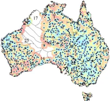
Figure 4-18 The difference between the expected proportions above cut-offs (Ni and Co), calculated from realisations, and real proportions above cut-offs, calculated from the validation data ... 108 Figure 5-1 (a) Major crustal blocks of Australia (coloured and numbered). The line styles of the MCB boundaries reflect the confidence level in their position/existence (solid thick: high; solid thin: moderate; dashed: low; dot-dashed: none). (b) Surface geology and the geological regions of Australia. The NGSA sample site locations are shown as black dots on both maps. Sources: Blake and Kilgour ( 1998), Caritat and Cooper (2011), Korsch and Doublier (2016), Nakamura and Milligan (2015), Raymond (2012). Modified after Grunsky et al. (2017) ... 129

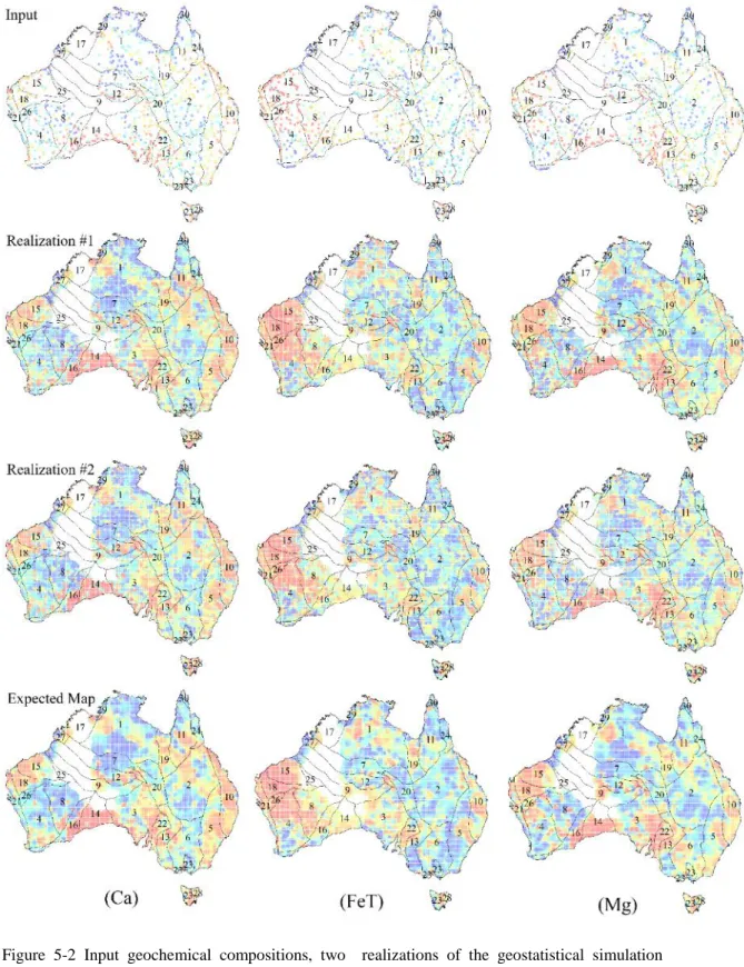
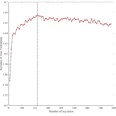
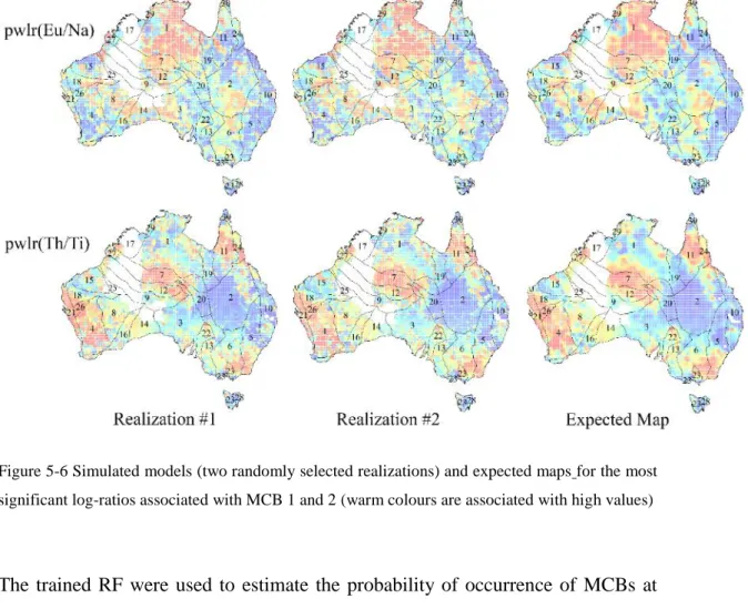
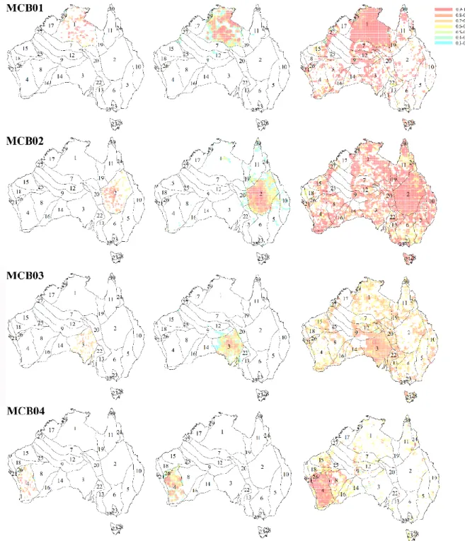
Figure 5-2 Input geochemical compositions, two realizations of the geostatistical simulation procedure and expected map for three major components Ca, total Fe and Mg (warm colours are associated with high values) ... 131 Figure 5-3 Conditional total compositional variation, a means to assess the spatial uncertainty of the geochemical compositions (warm colours are associated with high uncertainty and black dots are the location of samples) ... 132 Figure 5-4 Recursive feature elimination with resampling to identify the most important subset of log-ratios ... 133 Figure 5-5 The top 30 most informative log-ratios for classification of all MCBs (the significance of selected log-ratios is decreasing from the top to bottom of the chart) ... 133 Figure 5-6 Simulated models (two randomly selected realizations) and expected maps for the most significant log-ratios associated with MCB 1 and 2 (warm colours are associated with high values) ... 135 Figure 5-7 Maps of minimum (first column), expected (middle column) and maximum (last column) probability of occurrence for MCB 1 to 4 ... 136

Figure 5-8 Conditional total variation of all simulated MCBs (warm colours show high values) ... 137

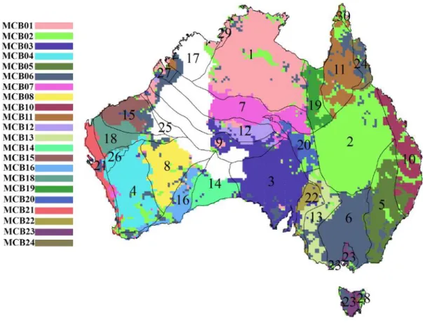
Figure 5-9 Map of most probable MCBs ... 138 Figure 5-10 Post-glacial peat-covered areas; adapted from McKinley et al. (2018) ... 139

(17)

xvi

Figure 5-11 Conditional total compositional variation (warm colours are associated with high values and black polygons are peat covered areas) ... 140 Figure 5-12 Recursive feature elimination with resampling to identify the most important subset of log-ratios (Northern Ireland Tellus Survey data) ... 141 Figure 5-13 The top 30 most informative log-ratios for discrimination of peat covered areas (the significance of selected log-ratios is decreasing from the top to bottom of the chart) ... 142 Figure 5-14 Simulated model (two randomly selected realizations) and expected map of the most significant log-ratio (pwlr (Y/filler)) for discrimination of peat covered areas (warm colours are associated with high values and black polygons are peat covered areas) ... 143 Figure 5-15 Maps of minimum, expected and maximum probability of occurrence for peat covered areas ... 145 Figure 5-16 Conditional total variation of simulated peat covered areas (warm colours are associated with high values and black polygons are peat covered areas) ... 146 Figure 5-17 Map of most probable peat covered areas (shown by red colour) ... 147

(18)

xvii

List of Tables

Table 2-1 DS parameters for the synthetic case study ... 35

Table 2-2 Total accuracy and sensitivity of DS for predicting true geological domains ... 42

Table 2-3 Descriptive statistics of global Aitchison distance of simulated compositions from validation compositions ... 43

Table 2-4 Selected DS parameters for the real case study ... 48

Table 3-1 Descriptive statistics. ... 65

Table 3-2 Parameters of variogram models of GRFs for the plurigaussian model (the anisotropy ranges are long, middle, and short range respectively). ... 66

Table 3-3 Variogram model parameters for the MAF factors derived from conditional Gaussian data (the anisotropy ranges are long, middle, and short range respectively). ... 68

Table 4-1 Proposed methods and the related features ... 87

Table 4-2 Ore mineralogy of different geological units at MME ... 89

Table 4-3 Proportions of rock types ... 96

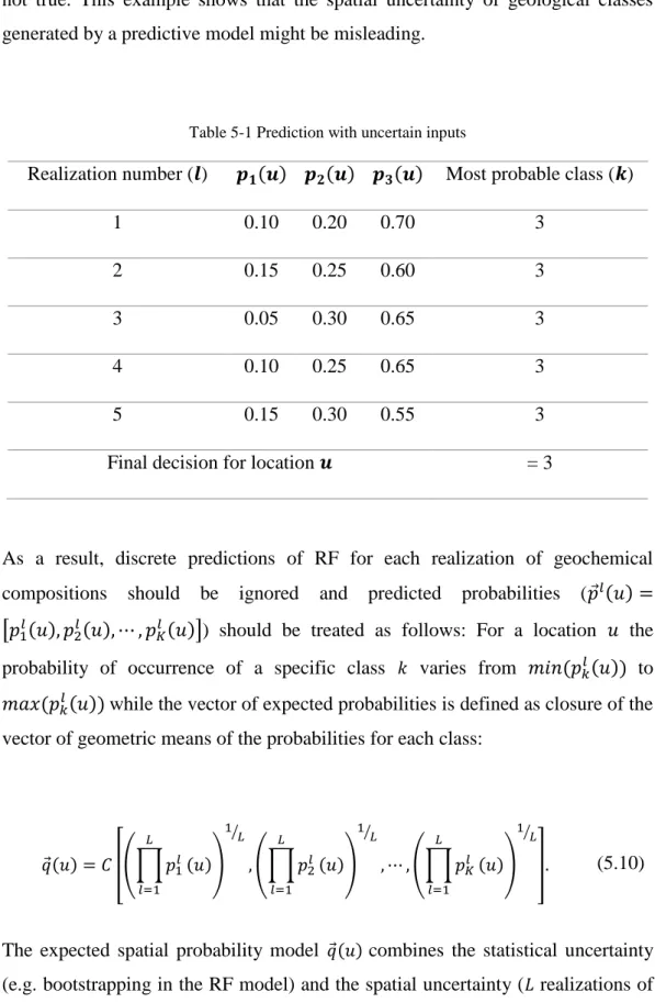
Table 5-1 Prediction with uncertain inputs ... 126

Table 5-2 The top 5 most important log-ratios (from left to right) associated with each MCB ... 134

(19)

Chapter 1

1.

General Introduction

1

1.1 Research background

In many geoscience applications such as evaluation of mineral resources, characterization of oil reservoirs, hydrology of groundwater, and contaminated site characterization and remediation, spatial uncertainty modelling and prediction of regionalized variables from various sample spaces (e.g. continuous and categorical) is required. Some of these variables are discrete or qualitative such as rock types, soil types, land uses, alteration or mineralization and some of them are continuous or quantitative such as mineral grade, porosity, permeability, water or oil saturation, and pollutant concentration. Several geostatistical models have been developed for the spatial modelling of categorical or continuous variables (Chilès and Delfiner 2012; Deutsch and Journel 1998; Goovaerts 1997; Wackernagel 2003), but for the joint modelling of such data little has been done because of the difficulties of integrated multivariate modelling of data of different characteristics. As the spatial distributions of these multivariate data are often interdependent, separate modelling of them is insufficient (Emery and Silva 2009; Maleki and Emery 2015; Talebi et al. 2017; van den Boogaart et al. 2018). Multivariate continuous data in the form of percentages, proportions, frequencies, and concentrations are common in geosciences (e.g. geochemical or mineralogical data, proportions of rock types in a mining block, and proportions of soil types or land uses in a study area). Such data are compositional in their nature which means they are non-negative and bounded, representing some parts of a whole (Aitchison 1982; Aitchison 1986). Compositional data carry just relative information and the constant sum constraint forces at least one covariance to be negative inducing spurious statistical and spatial correlations (Aitchison 1986; Pawlowsky-Glahn et al. 2015; Pawlowsky‐Glahn and Buccianti 2011; Tolosana-Delgado 2006; van den Boogaart and Tolosana-Delgado 2013). As a result, classical (geo)statistical techniques should not be implemented on the original compositional data (Pawlowsky-Glahn and Egozcue 2016; Pawlowsky-Glahn and Olea 2004; Tolosana-Delgado 2006). The spatial analysis of

(20)

2

compositional data is an open area of research (Buccianti and Grunsky 2014; McKinley et al. 2016; Mueller et al. 2014; Mueller et al. 2017; Pawlowsky-Glahn and Egozcue 2016; Tolosana-Delgado et al. 2015a; Tolosana-Delgado et al. 2016; Tolosana-Delgado et al. 2015b; Tolosana-Delgado and van den Boogaart 2014; van den Boogaart et al. 2017; van den Boogaart and Tolosana-Delgado 2013; van den Boogaart et al. 2018). Demands for spatial modelling of such constrained multivariate data with different categorical variables simultaneously add more complexity (Talebi et al. 2017; van den Boogaart et al. 2018). To jointly model such mixed and constrained data, and to reproduce complex relationships between them, existing geostatistical techniques need to be modified and adapted.

1.2 Literature review

Spatial modelling of compositional data

A random vector with non-negative components representing parts of a whole which carries relative information (ratios between components carry information and not the absolute values) is a composition (Aitchison 1982, 1986). Statistical analysis of compositional data and the log-ratio approaches were first introduced by Aitchison (1982, 1986). Many of the regionalized variables predicted via geostatistical approaches are compositional such as ore grades, mineral and geochemical data, contaminants, porosity, saturation, and many other petro-physical variables. Spurious spatial correlations between such regionalized compositional variables, were first recognised by Pawlowsky-Glahn (1984). Spurious correlation is generated when compositional data are treated as real data, with the usual Euclidean geometry (Pawlowsky-Glahn and Egozcue 2016). Indeed, compositions are equivalence classes, so a closed composition is just a representation (Pawlowsky-Glahn et al., 2015). The result of compositional analyses under the assumption of equivalence classes are valid for any other representations and are fully addressed via the implementation of log-ratio transformations. The first attempt to construct spatial models of regionalised compositions was the implementation of the additive log-ratio (alr) transformation and cokriging the log-ratios (Aitchison, 1982; Aitchison, 1986; Pawlowsky-Glahn and Olea, 2004). However, this approach has some limitations. For instance,

(21)

3

computation of variances and covariances using the alr coordinates may be problematic (See Pawlowsky-Glahn and Olea, (2004) for more information). Orthogonal projection of compositional data into real (Cartesian coordinates) space leads to easy use of many (geo)statistical algorithms (Mateu-Figueras et al., 2011). Nowadays analysis of compositional data is commonly summarised by working on coordinates (projection to orthogonal coordinates known as isometric log-ratio transformation (Egozcue et al. 2003)), where compositional data are projected to real space (unbounded and unconstrained) and multivariate geostatistical algorithms can be implemented for spatial modelling purposes, followed by back-transformation to compositional space.

In the case of geostatistical simulation, having a multivariate Gaussian distribution is a primary assumption for experimental data (log-ratios in the case of compositional data). Several methods have been proposed to address this assumption. The results of geostatistical simulation achieved by simple methods of transformation to normal space, like the normal score transformation (Deutsch and Journel 1998), or in the case of high dimensional data with complicated relationships, advanced transformation methods like the stepwise conditional transformation (Leuangthong and Deutsch 2003) and projection pursuit method (Barnett et al. 2014), are not independent of the choice of log-ratio transformation. In the geostatistical treatment of compositional data, it is desirable to have invariant results in each step (Tolosana-Delgado 2006). To transform the log-ratios into a multivariate standard normal distribution, van den Boogaart et al. (2017) proposed a method based on a continuous affine-equivariant multivariate kernel density deformation (flow anamorphosis) which is quite useful for joint geostatistical simulation of compositional data. Several applications have shown that the transformed data via flow anamorphosis are not only multivariate normal but often exhibit absence of spatial cross-correlation which make the geostatistical simulation of such orthogonal factors, more straightforward (Mueller et al. 2017; van den Boogaart et al. 2017). Flow anamorphosis is also capable of reproducing complex patterns in input data including presence of outliers, presence of several populations, nonlinearity, and heteroscedasticity.

Although many studies have been conducted on the spatial modelling of regionalized compositional data (Buccianti and Grunsky 2014; Grunsky et al. 2017;

(22)

4

Grunsky et al. 2014; McKinley et al. 2018; McKinley et al. 2016; Mueller et al. 2014; Pawlowsky-Glahn and Egozcue 2016; Pawlowsky-Glahn and Olea 2004; Delgado and McKinley 2016; Delgado et al. 2016; Tolosana-Delgado et al. 2015b; Tolosana-Tolosana-Delgado and van den Boogaart 2013; Tolosana Delgado 2006; van den Boogaart and Tolosana-Delgado 2013), few of these studies considered the spatial relationships between regionalized compositions and the other dependent categorical information (Talebi et al. 2017; van den Boogaart et al. 2018). The dependent categorical data such as rock type, soil type, mineralization type, and crustal blocks are related (statistically and spatially) to the compositional data. The multi-population characteristic of the input data is generally related to a dependent categorical variable. Most of the time, the input data are separated into purer subpopulations and geostatistical analyses are implemented on these subsets independently (this process is commonly known as domaining). Another approach is to apply nonstationary geostatistical algorithms. However, multivariate geostatistical simulation via flow anamorphosis introduces new ways for spatial modelling of complex compositional data. For instance, the need for domaining prior to geostatistical modelling (to fulfil stationarity assumptions) due to multi-population characteristic of input data may become unnecessary in some applications. More studies are needed to assess the potential of geostatistical simulation of compositional data via orthogonal projection (isometric log-ratio transformation) and flow anamorphosis. The complex relationships between compositional and categorical data should be honoured in the estimated or simulated models. More studies are needed to assess the effect of one or more dependent (statistically and spatially) categorical variable on spatial modelling of compositional data.

Two-point geostatistical modelling of mixed data

Two-point geostatistical algorithms are based on the moments up to second order (variogram, covariance and variance). The spatial autocorrelation (spatial variation for a single variable) and cross-correlation (spatial variation between different variables) are considered via calculating experimental (cross)variograms and fitting models to them (Chilès and Delfiner 2012; Isaaks and Srivastava 1989). As an early

(23)

5

solution to joint spatial modelling of multivariate data with different characteristics, modellers suggested the use of a deterministic model based on one categorical variable and prediction of continuous data within each category separately (Dowd 1986; Duke and Hanna 2001; Rossi and Deutsch 2014; Sinclair 1998; Sinclair and Blackwell 2002). Although this model is simple to apply, it does not consider the uncertainty in the layout of the categories (e.g. geological domains). In this approach geologists have to delineate the exact shape of each layout based on experimental data and their interpretation of earth science processes. Unfortunately, very few of such processes are understood well enough to allow modellers to use deterministic models (Isaaks and Srivastava 1989). As the experimental data become sparse and geology becomes more complex the likelihood of misclassification in the spatial model of categorical variable increases dramatically.

A solution to this shortcoming is to use probabilistic models to simulate the categorical data distributions in space and predict the continuous data in each simulated category independently (Alabert and Massonnat 1990; Boucher and Dimitrakopoulos 2012; Dubrule 1993; Jones et al. 2013; Roldão et al. 2012; Talebi et al. 2016). This method is known as a cascade or hierarchical approach. In this approach geostatistical simulations for categorical data are used to improve the domain definition and quantify the uncertainty in the position of their boundaries by generating multiple realizations. Many simulation models are available for simulating categorical data including sequential indicator (Deutsch 2006; Journel and Alabert 1990; Journel and Gomez-Hernandez 1993), Boolean (Lantuéjoul 2002), truncated Gaussian (Galli et al. 1994; Matheron et al. 1987), plurigaussian (Armstrong et al. 2011), and multipoint simulation (Mariethoz and Caers 2015; Strebelle 2002) and therefore a method suited to the specific data can be selected at this step. Although the cascade approach is simple and has powerful tools for measuring uncertainty in categorical and continuous data, it has some substantial drawbacks. The method does not consider the spatial relationship of continuous and categorical data and also does not take into account the spatial dependence of continuous data across domain boundaries and in turn generates abrupt transitions when crossing boundaries which is not always the case in practice (Kim et al. 2005; Larrondo et al. 2004; Ortiz and Emery 2006; Talebi et al. 2015; Tolosana-Delgado et al. 2014; Wilde and Deutsch 2012).

(24)

6

To account for the continuity of the continuous data across domain boundaries and the uncertainty in the spatial extent of these domains, a probabilistic approach can be applied based on geostatistical simulation of the categorical data and on the calculation of their probabilities of occurrence over the area of interest. These probabilities are then used for weighting the predictions of continuous data to derive predictions associated with each domain (Emery and González 2007a; Emery and González 2007b; Talebi et al. 2015). This approach is appropriate for reproducing gradual transitions in the realization of continuous variables across boundaries (soft boundaries). However, it provides just one scenario of variation for the continuous data in the area of interest which is not useful for uncertainty modelling and risk assessment purposes. On the other hand, the final integrated map may be over-smoothed due to the averaging nature of this algorithm.

To take into account the spatial correlations of continuous and categorical data and spatial correlations of continuous data across boundaries, and as well as considering the uncertainty of categorical and continuous data distributions simultaneously, one approach is to co-simulate these two kinds of variables. Bahar and Kelkar (2000) proposed a co-simulation approach in which one categorical variable is generated by truncating one Gaussian random field and one continuous variable by transforming an independent Gaussian random field. For reproducing the spatial dependencies of two variables they proposed a transformation function for the second Gaussian random field conditionally on the simulated domain. An alternative to this approach is to use a truncated Gaussian random field for categorical data and a correlated Gaussian random field for continuous data (Dowd 1994; Dowd 1997; Freulon et al. 1990). However, the two aforementioned models may have some shortcomings when multivariate data with complex spatial relationships are considered. These methods use several simplifications including using a restrictive coregionalization model for two Gaussian random fields, transforming the categorical variables into continuous Gaussian data without considering the effects of conditional continuous variables, assuming spatially ordered sequences of categories and using one model of anisotropy for them (therefore this model is not practical for modelling complex relationships of geological domains). A more general approach is to use an extension of multivariate Gaussian and plurigaussian models simultaneously (Cáceres and Emery 2010;

(25)

7

Emery and Silva 2009; Maleki and Emery 2015). In this model continuous data are associated with a multivariate Gaussian random field and categorical data with the truncation of one or more Gaussian random fields. Further, it is assumed that all Gaussian random fields are spatially cross-correlated so it is possible to reproduce the dependencies between the categorical and continuous data. This method offers several advantages such as accounting for the uncertainty in the spatial layout of the boundaries between different categories, the ability to reproduce soft boundaries and considering the spatial dependencies between categorical and continuous data. The model also has the ability to incorporate non-stationarity in the categorical data (Maleki and Emery 2017) and can be generalized to the joint simulation of several continuous and categorical variables by adding more Gaussian random fields. Although the method is very flexible and has several advantages over earlier models, there are still some shortcomings. This approach follows a co-simulation based on defining a linear model of coregionalization (LMC) to jointly simulate multivariate data. Simplicity of modelling and verification of the admissibility make the LMC a popular means for defining the spatial relationships of multivariate data (Goulard and Voltz 1992). However, defining symmetrical cross-covariances and using the same structure in the cross-covariance and related variables are shortcomings which decrease the flexibility of the method since in geoscience applications variables are cross-correlated with different support and different spatial behaviour.

To address the problems of LMC, Marcotte (2012) offered a generalized of LMC (GLMC) in which the observed variables are considered as linear combinations of few primary independent variables and some other variables which are deterministic functions of primary variables. A more flexible technique would be, in the multivariate case, the non-LMC approach. Through the use of a non-LMC approach any number of variables, with any number of components for each structure can be considered. Furthermore each component can be isotropic or anisotropic (Marcotte 2015).

High-dimensional data are very common in geosciences and as the number of variables and simulation domain increase, co-simulation approaches based on an LMC or non-LMC will need considerable computer processing to solve large systems of equations per simulated node. An alternative is to decompose the

(26)

8

variables under study into factors which are uncorrelated spatially. Such orthogonal factors can then be simulated independently. Statistical and spatial relationships between variables can be reimposed on the simulated model afterward. This approach for joint simulation offers better accuracy and computational efficiency as the number of attributes being simulated increases. Principal component analysis (PCA) (Davis 1987; Wackernagel 2003), minimum/maximum autocorrelation factors (MAF) (Bandarian et al. 2008; Desbarats and Dimitrakopoulos 2000; Rondon 2012; Vargas-Guzmán and Dimitrakopoulos 2003), and U-WEDGE (Mueller and Ferreira 2012) are some examples of decorrelation methods. As these decorrelation methods have not been developed enough for reproduction of complex relationships such as non-linearity, constraints, or heteroscedasticity, using a chained transformation might produce more satisfactory results (Barnett and Deutsch 2012; Barnett et al. 2014; Mueller et al. 2014). However, a sensitivity analysis must be done to find the optimum order of transformations in a chain. Furthermore, the aforementioned spatial decorrelation techniques were developed for joint simulation of multivariate continuous variables and none of them considered the effects of other dependent regionalized categorical variables. Spatial prediction and uncertainty modelling of a mixture of regionalized continuous and categorical variables is common in many geoscience applications. New spatial decorrelation techniques have to be developed with the ability to jointly simulate many dependent (statistically and spatially) continuous and categorical variables. Such techniques should be able to address the compositional nature of some continuous variables.

Multiple-point geostatistical modelling of mixed data

Two-point geostatistical techniques are constrained by using 2-point statistics only and are inefficient in reproducing complex spatial structures and patterns (Guardiano and Srivastava 1993; Mariethoz and Caers 2015; Strebelle 2000; Strebelle 2002). Such complex spatial patterns might not be properly modelled using traditional two point spatial statistics such as variograms (Journel and Zhang 2006). Multiple-point geostatistical simulation (MPS) techniques capture spatial patterns from so-called training images or training data. Using higher order

(27)

9

statistics makes the MPS algorithms capable of reproducing complex spatial patterns. However, large and representative training images or training data with desirable resolution are needed to model the spatial uncertainties properly. Many MPS algorithms have been developed in the recent years, however few of them are capable of running co-simulation of mixed data (Mariethoz et al. 2010; Peredo and Ortiz 2011; van den Boogaart et al. 2018).

A spatial predictive model was developed by van den Boogaart et al. (2018) which combines a multipoint geostatistical algorithm with a new form of distributional regression to estimate conditional distributions. The algorithm is capable of jointly simulating dependent spatial variables from various sample spaces (e.g.

compositional, distributional, geometrical, and categorical). However,

computational effort is substantial. The algorithm needs further development to simulate large mineral deposits or petroleum reservoirs. MPS algorithms for joint simulation of compositional and categorical data need to be developed or adapted which are easy to implement and fast enough to simulate many dependent variables on large simulation grids. Among the MPS techniques, the Direct Sampling (DS) technique (Mariethoz et al. 2010) is well suited to the co-simulation of mixed data since an explicit estimation of a model of co-dependence is not required, multivariate spatial patterns of different sizes are captured without the need to define a search template of specific size and geometry, and spatial patterns of different scales are captured without the need for a multigrid search strategy. However, DS is a distance based technique and requires measuring the distance between the spatial data events, which is problematic in the case of compositional data. Distances should not be measured from the original compositional data (data in form of proportions, percentages, probabilities, frequencies, and concentrations). The lack of sub-compositional coherence of Euclidean distances (Pawlowsky-Glahn et al. 2015) and the fact that these distances are massively dominated by the major components of the system (while the component of interest might be one of the small components) are some of the reasons why DS should not be implemented on the original compositional data, but on suitably transformed data. Other metrics for measuring the distance between spatial compositional patterns should be developed and implemented (such as Aitchison distance) or compositional data should be transformed to real space via an isometric transformation prior to

(28)

10

simulation via DS. New metrics should be defined to assess the performances of DS to simulate the compositional random function and spatial compositional patterns.

Application of machine learning algorithm for compositional data modelling

Over the past few years, many studies have involved the use of machine learning algorithms (MLAs) to explore the compositional patterns as footprints for geoscience process discovery analysis (Caritat et al. 2017; Carranza 2017; Grunsky et al. 2017; Grunsky et al. 2014; McKinley et al. 2018; Tolosana-Delgado et al. 2015a; Tolosana-Delgado and van den Boogaart 2014). Few of these studies have addressed the spatial correlations between geospatial data and the associated spatial uncertainty. Most of the machine learning algorithms are non-spatial techniques, which means they do not consider the multivariate spatial relationships between variables. As a result, the probability maps generated via MLAs cannot be accepted as the model of spatial uncertainty. In geostatistics, spatial relationships are taken into account via means such as second order ((cross)variograms) and/or higher order statistics (training images). In many applications of MLAs for spatial data, uncertainty associated with the input spatial data is ignored. However, this uncertainty can be incorporated into the machine learning algorithms by combining these non-spatial learners with geostatistical simulation. Each realization of random function can be used as an input (new observation) to a trained classifier. Ensemble classifiers which combine many simple learners (e.g. built from bootstrap samples) are preferable due to their stability, better predictive performance, ability to measure the performance and to select the most significant features internally (Breiman 1996). The estimated probabilities of different classes (e.g. rock or soil type as a categorical response variable) for all geostatistical realizations should be combined afterward. Such combination integrates elements of statistical and spatial uncertainties. However, care should be taken when combining these estimated probabilities to avoid any systematic bias. The new combined spatial uncertainty model can be used further to predict most probable classes. The proposed algorithm should address the compositional nature of data. Due to the high-dimensional

(29)

11

characteristics of compositional features (log-contrasts), developing a compositionally compliant feature selection will be useful for geoscience process discoveries.

1.3 Research objectives

The main objective of this research is to develop approaches for the joint modelling of regionalized compositional and categorical data. This study aims to address the following objectives:

1. To adapt the implementation of the direct sampling technique for the joint simulation of compositional and categorical data, and to introduce new metrics to evaluate the simulated compositional random function.

2. To develop a spatial decorrelation technique for joint two-point geostatistical simulation of high-dimensional continuous and categorical data. The compositional nature of some multivariate continuous variables will be addressed properly within the proposed algorithm.

3. To assess the capability of geostatistical simulation of complex regionalized compositional data via orthogonal projection (isometric log-ratio transformation) and flow anamorphosis. Effects of a dependent regionalized categorical variable on the predicted compositions will be assessed.

4. To adapt the implementation of machine learning algorithms (non-spatial ensemble classifiers in this study) to address the spatial uncertainty of input data. This will be achieved by combining the non-spatial classifiers (e.g. random forest) with geostatistical simulation. The estimated probabilities for several realizations of random function will be combined to integrate elements of statistical and spatial uncertainties. The new model of spatial uncertainty will be used further for prediction of various classes (e.g. rock or soil type as a categorical response variable). A coherent compositional feature selection will be introduced. The compositional nature of data will be addressed properly within all steps of proposed technique.

(30)

12

5. To assess the capability and performance of the developed techniques via implementing on real geoscientific case studies.

For situations where large and representative training images are available, multiple-point geostatistical methods are preferable. Due to the complexity of multivariate mixed and constrained geospatial data, the implementation of direct sampling technique is adapted for joint simulation of compositional and categorical data. The applicability and usefulness of the proposed algorithm is tested on one synthetic and one real case study.

The second objective of this PhD research is to develop a spatial decorrelation technique for joint simulation of high-dimensional continuous and categorical data. This method is appropriate for modelling projects where large and representative training images with proper resolution are not available. Along with generating predictions, the spatial uncertainty of regionalized continuous and categorical variables will be evaluated. The compositional nature of some multivariate continuous variables will be considered. The new method will be tested on a real mining case study.

Advanced geostatistical simulation of compositional data via orthogonal projection (isometric log-ratio transformation) and flow anamorphosis will be investigated. Ability of such algorithm to reproduce complex patterns such as presence of outliers, multi-population characteristic, and nonlinearity will be assessed. Multi-population characteristic and/or non-stationarity phenomenon might be related to a dependent categorical variable (e.g. geological units). Implementing such advanced geostatistical simulation technique may make the need for domaining and/or handling of non-stationarity unnecessary in some applications and situations. Effects of a dependent regionalized categorical variable on the whole process of spatial simulation of compositions will be investigated. The new method will be tested on a real mining case study.

Finally, to utilize the capability of machine learning algorithms to explore complex multivariate patterns and to select and rank features in a spatial framework, a hybrid spatial predictive model is developed based on the combined use of advanced geostatistical simulation techniques and machine learning algorithms. The spatial uncertainty of input compositional data is fully addressed. The new combined

(31)

13

spatial uncertainty model is used further for class prediction. A fully compositional feature selection is introduced. The developed hybrid model is used for surficial and deep earth material prediction through two real case studies.

1.4 Thesis structure

This thesis is presented and organised as “Thesis with publication” format1; and is structured in chapters as follows:

Chapter 1 presents the background of this PhD research and literature overview. The objectives of the research and the structures of the thesis are discussed in separate subsections.

Chapter 2 presents the developed method for joint simulation of compositional and categorical data via the direct sampling technique. The potential of the developed algorithm to improve mineral resource confidence is explored via one synthetic and one real mining case study.

Chapter 3 introduces a hybrid model for joint simulation of high-dimensional continuous and categorical variables in two-point geostatistical framework. The model is tested on a real mining case study.

Chapter 4 explores various approaches to geostatistical simulation of regionalized compositions consisting of several populations. Applications of such techniques to mineral resource evaluation are investigated.

Chapter 5 introduces a new workflow for implementation of a spatial predictive model (a hybrid of geostatistical simulation and machine learning). The potential of the new model is investigated through its application to surficial and deep earth material prediction from geochemical compositions.

1_{“Thesis with publication” format is an acceptable format of thesis for postgraduate research at}

ECU policy. The current thesis has been written based on the guideline provided at

http://www.ecu.edu.au/GPPS/policies_db/policies_view.php?rec_id=0000000434. In this format,

the submitted thesis can consist of publications that have already been published, are in the process of being published, or a combination of these.

(32)

14

Chapter 6 presents the general discussions on the developed techniques. Pros and cons of the developed techniques and the area of their application are discussed in this chapter.

Chapter 7 covers the overall conclusions of this PhD thesis and further recommendations.

1.5 Chapter references

Aitchison J (1982). The statistical analysis of compositional data. Journal of the Royal Statistical Society, Series B (Methodological), 44, 139-177.

Aitchison J (1986). The statistical analysis of compositional data. London, UK, Chapman & Hall Ltd.

Alabert FG, Massonnat GJ (1990). Heterogeneity in a complex turbiditic reservoir: Stochastic modelling of facies and petrophysical variability. SPE Annual Technical Conference and Exhibition, https://doi.org/10.2118/20604-MS. Armstrong M et al. (2011). Plurigaussian Simulations in Geosciences. Berlin

Heidelberg, Berlin, Heidelberg, Springer, https://doi:10.1007/978-3-642-19607-2_3.

Bahar A, Kelkar M (2000). Journey from well logs/cores to integrated geological and petrophysical properties simulation: A methodology and application.

Society of Petroleum Engineers, https://doi.org/10.2118/66284-PA.

Bandarian EM, Bloom LM, Mueller U (2008). Direct minimum/maximum autocorrelation factors within the framework of a two structure linear model

of coregionalisation. Computers&Geosciences, 34, 190-200,

https://doi.org/10.1016/j.cageo.2007.03.015.

Barnett RM, Deutsch CV (2012). Practical implementation of non-linear transforms for modeling geometallurgical variables. In: Abrahamsen P, Hauge R, Kolbjørnsen O (eds), Geostatistics Oslo 2012, vol 17. Quantitative Geology

and Geostatistics. Netherlands, Springer, pp 409-422,

https://doi:10.1007/978-94-007-4153-9_33.

Barnett RM, Manchuk JG, Deutsch CV (2014). Projection pursuit multivariate

transform. Mathematical Geosciences, 46, 337-359,

https://doi:10.1007/s11004-013-9497-7.

Boucher A, Dimitrakopoulos R (2012). Multivariate block-support simulation of the Yandi iron ore deposit, Western Australia. Mathematical Geosciences, 44, 449-468, https://doi:10.1007/s11004-012-9402-9.

Breiman L (1996). Bagging predictors. Machine Learning, 24, 123-140.

Buccianti A, Grunsky E (2014). Compositional data analysis in geochemistry: Are we sure to see what really occurs during natural processes? Journal of Geochemical Exploration, 141, 1-5 https://doi.org/10.1016/j.gexplo.2014.03.022.

Cáceres A, Emery X (2010). Conditional co-simulation of copper grades and lithofacies in the Rio Blanco-Los Bronces copper deposit. In: Castro R, Emery X, Kuyvenhoven R (eds), Proceedings of the IV international

(33)

15

conference on mining innovation MININ 2010, Santiago, Chile, Gecamin Ltd, pp 311–320.

Caritat P de, Main PT, Grunsky EC, Mann AW (2017). Recognition of geochemical footprints of mineral systems in the regolith at regional to continental scales.

Australian Journal of Earth Sciences, 64, 1033-1043, https://doi:10.1080/08120099.2017.1259184.

Carranza EJM (2017). Natural Resources Research publications on geochemical anomaly and mineral potential mapping, and introduction to the special issue of papers in these fields. Natural Resources Research, 26, 379-410, https://doi:10.1007/s11053-017-9348-1.

Chilès, J. P., Delfiner, P. (2012). Geostatistics: modeling spatial uncertainty. New York: Wiley.

Davis M (1987). Production of conditional simulations via the LU triangular decomposition of the covariance matrix. Mathematical Geology, 19, 91-98, https://doi:10.1007/BF00898189.

Desbarats AJ, Dimitrakopoulos R (2000). Geostatistical simulation of regionalized

pore-size distributions using min/max autocorrelation factors.

Mathematical Geology, 32, 919-942, https://doi:10.1023/A:1007570402430.

Deutsch CV (2006). A sequential indicator simulation program for categorical variables with point and block data: BlockSIS. Computers & Geosciences, 32, 1669-1681, http://dx.doi.org/10.1016/j.cageo.2006.03.005.

Deutsch CV, Journel AG (1998). GSLIB: Geostatistical software library and user's guide. New York, Oxford University Press.

Dowd PA (1986). Geometrical and geological controls in geostatical estimation and

orebody modelling. Proceedings of the 19th APCOM Conference: Society

of Mining Engineers, Inc., Littletown Colorado, p 81–89.

Dowd PA (1994). Geological controls in the geostatistical simulation of hydrocarbon reservoirs. Arabian Journal for Science and Engineering, 19, 237-247.

Dowd PA (1997). Structural controls in the geostatistical simulation of mineral deposits. Paper presented at the Baafi EY, Schofield NA (Eds.),

Geostatistics Wollongong, Kluwer Academic, Dordrecht.

Dubrule O (1993). Introducing more geology in stochastic reservoir modelling. In: Soares A (ed), Geostatistics Tróia, vol 5. Quantitative Geology and Geostatistics. Springer Netherlands, pp 351-369.

Duke JH, Hanna PJ (2001). Geological interpretation for resource modelling and estimation. Monograph Series, Australasian Institute of Mining and Metallurgy, 23, 147-156.

Egozcue JJ, Pawlowsky-Glahn V, Mateu-Figueras G, Barceló-Vidal C (2003). Isometric logratio transformations for compositional data analysis.

Mathematical Geology, 35, 279-300.

Emery X, González KE (2007a). Incorporating the uncertainty in geological boundaries into mineral resources evaluation. J Geol Soc India, 69(1), 29– 38.

Emery X, González KE (2007b). Probabilistic modelling of lithological domains and it application to resource evaluation. Journal of the Southern African Institute of Mining and Metallurgy, 107, 803-809.

(34)

16

Emery X, Silva DA (2009). Conditional co-simulation of continuous and categorical variables for geostatistical applications. Computers & Geosciences, 35, 1234-1246.

Freulon XD, Fouquet C, Rivoirard J (1990). Simulation of the geometry and grades of a uranium deposit using a geological variable. In: International Symposium on Applications of Computers and Operations Research in the Mineral Industry, Technische Universität Berlin, Berlin, pp 649–659. Galli A, Beucher H, Le Loc’h G, Doligez B, Group H (1994). The pros and cons of

the truncated gaussian method. In: Geostatistical Simulations, vol 7. Quantitative Geology and Geostatistics. Netherlands, Springer, pp 217-233. Goovaerts P (1997). Geostatistics for Natural Resources Evaluation. Applied

Geostatistics. Oxford University Press.

Goulard M, Voltz M (1992). Linear coregionalization model: Tools for estimation and choice of cross-variogram matrix. Mathematical Geology, 24, 269-286. Grunsky EC, de Caritat P, Mueller UA (2017). Using surface regolith geochemistry to map the major crustal blocks of the Australian continent. Gondwana Research, 46, 227-239.

Grunsky EC, Mueller UA, Corrigan D (2014). A study of the lake sediment geochemistry of the Melville Peninsula using multivariate methods: Applications for predictive geological mapping. Journal of Geochemical Exploration, 141, 15-41.

Guardiano FB, Srivastava RM (1993). Multivariate Geostatistics: beyond bivariate moments. In: Soares A (ed), Geostatistics Tróia ’92: Volume 1. Netherlands, Springer, Dordrecht, pp 133-144.

Isaaks EH, Srivastava RM (1989). An introduction to applied geostatistics. Oxford University Press.

Jones P, Douglas I, Jewbali A (2013). Modeling combined geological and grade uncertainty: Application of multiple-point simulation at the Apensu gold deposit, Ghana. Mathematical Geosciences, 45, 949-965.

Journel AG, Zhang T (2006). The necessity of a multiple-point prior model.

Mathematical Geology, 38, 591-610.

Journel AG, Alabert FG (1990). New method for reservoir mapping. SPE-18324-PA, 42, 2012-2218.

Kim HM, Mallick BK, Holmes CC (2005). Analyzing nonstationary spatial data using piecewise gaussian processes. Journal of the American Statistical Association, 100, 653-668.

Lantuéjoul C (2002). Geostatistical simulation. Springer-Verlag Berlin Heidelberg. Larrondo P, Leuangthong O, Deutsch CV (2004). Grade estimation in multiple rock

types using a linear model of coregionalization for soft boundaries. Paper presented at the Proceedings of the 1st international conference on mining innovation. Gecamin Ltd, Santiago, Chile.

Leuangthong O, Deutsch CV (2003). Stepwise conditional transformation for simulation of multiple variables. Mathematical Geology, 35, 155-173. Maleki M, Emery X (2015). Joint simulation of grade and rock type in a stratabound

copper deposit. Mathematical Geosciences, 47, 471-495.

Maleki M, Emery X (2017). Joint simulation of stationary grade and non-stationary rock type for quantifying geological uncertainty in a copper deposit.

(35)

17

Marcotte D (2012). Revisiting the linear model of coregionalization. In:

Geostatistics Oslo, Quantitative Geology and Geostatistics. Springer Netherlands, pp 67-78.

Marcotte D (2015). TASC3D: A program to test the admissibility in 3D of non-linear models of coregionalization. Computers & Geosciences, 83, 168-175. Mariethoz G, Caers J (2015). Multiple-Point geostatistics: Stochastic modeling

with training images. John Wiley & Sons, Ltd.

Mariethoz G, Renard P, Straubhaar J (2010). The direct sampling method to perform multiple-point geostatistical simulations. Water Resources Research, https://doi:10.1029/2008WR007621.

Mateu-Figueras, G., Pawlowsky-Glahn, V., Egozcue, J.J., (2011). The principle of working on coordinates. In: Pawlowsky‐Glahn V, and Buccianti A (eds.),

Compositional Data Analysis. https://doi.org/10.1002/9781119976462.ch3. Matheron G, Beucher H, de Fouquet C, Galli A, Guerillot D, Ravenne C (1987). Conditional simulation of the geometry of Fluvio-Deltaic reservoirs. Society of Petroleum Engineers, https://doi.org/10.2118/16753-MS.

McKinley JM, Grunsky E, Mueller U (2018). Environmental monitoring and peat assessment using multivariate analysis of regional-scale geochemical data.

Mathematical Geosciences, 50, 235-246.

McKinley JM et al. (2016). The single component geochemical map: Fact or fiction? Journal of Geochemical Exploration, 162, 16-28.

Mueller U, Ferreira J (2012). The U-WEDGE transformation method for multivariate geostatistical simulation. Mathematical Geosciences, 44, 427-448.

Mueller U, Tolosana-Delgado R, van den Boogaart KG (2014). Approaches to the simulation of compositional data – a nickel-laterite comparative case study. Paper presented at the Orebody Modelling and Strategic Mine Planning Symposium, Melbourne.

Mueller U, van den Boogaart KG, Tolosana-Delgado R (2017). A truly multivariate normal score transform based on lagrangian flow. In: Gómez-Hernández JJ, Rodrigo-Ilarri J, Rodrigo-Clavero ME, Cassiraga E, Vargas-Guzmán JA (eds.), Geostatistics Valencia 2016. Springer International Publishing, Cham, pp 107-118.

Ortiz JM, Emery X (2006). Geostatistical estimation of mineral resources with soft geological boundaries: a comparative study. The South African Institute of Mining and Metallurgy, 106, 577–584.

Pawlowsky-Glahn V, Egozcue JJ (2016). Spatial analysis of compositional data: A historical review. Journal of Geochemical Exploration, 164, 28-32.

Pawlowsky-Glahn V, Egozcue JJ, Tolosana-Delgado R (2015). Modelling and analysis of compositional data. John Wiley & Sons, Ltd.

Pawlowsky-Glahn V, Olea RA (2004). Geostatistical analysis of compositional data. Oxford University Press.

Pawlowsky‐Glahn V, Buccianti A (2011). Compositional data analysis: Theory and applications. John Wiley & Sons, Ltd.

Pawlowsky-Glahn V (1984). On spurious spatial covariance between variables of constant sum. Sci de la Terre Inf Geol, 21, 107-113.

Pawlowsky-Glahn V, Burger H (1992). Spatial structure analysis of regionalized compositions. Mathematical Geology, 24, 675-691.

(36)

18

Peredo O, Ortiz JM (2011). Parallel implementation of simulated annealing to reproduce multiple-point statistics. Computers & Geosciences, 37, 1110-1121.

Roldão D, Ribeiro D, Cunha E, Noronha R, Madsen A, Masetti L (2012). Combined use of lithological and grade simulations for risk analysis in iron ore, Brazil. In: Abrahamsen P, Hauge R, Kolbjørnsen O (eds.), Geostatistics Oslo 2012,

Quantitative Geology and Geostatistics. Springer Netherlands, pp 423-434. Rondon O (2012). Teaching aid: minimum/maximum autocorrelation factors for

joint simulation of attributes. Mathematical Geosciences, 44, 469-504. Rossi ME, Deutsch CV (2014). Mineral resource estimation. Springer, Dordrecht. Sinclair AJ (1998). Geological controls in resource/reserve estimation. Exploration

and Mining Geology, 7, 29-44.

Sinclair AJ, Blackwell GH (2002). Applied mineral inventory estimation. Cambridge University Press.

Strebelle S (2000). Sequential simulation drawing structures fro