Copyright © Taylor & Francis Group, LLC ISSN: 0747-4938 print/1532-4168 online DOI: 10.1080/07474930600713465
MULTIVARIATE STOCHASTIC VOLATILITY MODELS: BAYESIAN ESTIMATION AND MODEL COMPARISON
Jun Yu School of Economics and Social Sciences, Singapore Management University, Singapore
Renate Meyer Department of Statistics, University of Auckland, Auckland, New Zealand
In this paper we show that fully likelihood-based estimation and comparison of multivariate stochastic volatility (SV) models can be easily performed via a freely available Bayesian software called WinBUGS. Moreover, we introduce to the literature several new specifications that are natural extensions to certain existing models, one of which allows for time-varying correlation coefficients. Ideas are illustrated by fitting, to a bivariate time series data of weekly exchange rates, nine multivariate SV models, including the specifications with Granger causality in volatility, time-varying correlations, heavy-tailed error distributions, additive factor structure, and multiplicative factor structure. Empirical results suggest that the best specifications are those that allow for time-varying correlation coefficients.
Keywords DIC; Factors; Granger causality in volatility; Heavy-tailed distributions; MCMC; Multivariate stochastic volatility; Time-varying correlations.
JEL Classification C11; C15; C30; G12.
1. INTRODUCTION
Univariate stochastic volatility (SV) models offer powerful alternatives to ARCH-type models in accounting for both the conditional and the unconditional properties of volatility. Superior performance of univariate SV models over ARCH-type models is documented in Danielsson (1994) and Kim et al. (1998) in terms of in-sample fitting, and in Yu (2002) in terms of out-of-sample forecasting. As a result, the univariate SV model has been the subject of considerable attention in the literature; see, for example, Shephard (2005) for a collection of relevant studies on this topic.
Received November 22, 2004; Accepted November 12, 2005
Address correspondence to Jun Yu, School of Economics and Social Sciences, Singapore Management University, 90 Stamford Road, Singapore 178903; E-mail: [email protected]
There are both theoretical and empirical reasons that there is a great need to study multivariate volatility models. On the one hand, much of financial decision making, such as portfolio optimization, asset allocation, risk management, and asset pricing, clearly needs to take correlations into account. On the other hand, it is well known that financial market volatilities move together over time across assets. As a result, the multivariate ARCH models (MARCH) have attracted a lot of attention in modern finance theory and enjoyed voluminous empirical applications; see Bauwens et al. (2006) and McAleer (2005) for the literature review. Important contributions are Bollerslev et al. (1998), Diebold and Nerlove (1989), Bollerslev (1990), Engle et al. (1990), Engle and Kroner (1995), Braun et al. (1995), Engle (2002), Tse and Tusi (2002), among many others.
Compared to the MARCH literature, the literature on multivariate SV is much more limited (see McAleer, 2005, a partial review of the literature, and Asai et al., 2006, for a more detailed review), reflected by much fewer published papers on the topic to date (Aguilar and West, 2000; Chib et al., 2005; Danielsson, 1998; Harvey et al., 1994; Liesenfeld and Richard, 2003; Pitt and Shephard, 1999). Yet the multivariate SV models have certain statistical attractions relative to the MARCH models (Harvey et al., 1994). We believe there are several reasons that the multivariate SV models have had fewer empirical applications. Firstly, the multivariate SV models are more difficult to estimate. Although estimation is already an issue for the MARCH models, it is believed that estimation is more of an issue for the multivariate SV models. This is because, apart from the inherent problems of multivariate models, such as high dimensionality of the parameter space and the required positive semidefiniteness of covariance matrices, the likelihood function has no closed form for the multivariate SV model. Secondly, as a result of difficulties with parameter estimation, the computation of model comparison criteria becomes extensive and demanding. Thirdly, compared to abundant alternative specifications in MARCH, only a handful of multivariate SV model specifications have appeared in the literature. As a result, the existing multivariate SV models may not be able to describe some important stylized features of the data.
A variety of estimation methods have been proposed to estimate the SV models. Less efficient methods include GMM (Andersen and Sorensen, 1996; Melino and Turnbull, 1990), the quasi-maximum likelihood method (Harvey et al., 1994), and the method of the empirical characteristic function (Knight et al., 2002). Fully likelihood-based methods include the simulated maximum likelihood method (SML) (Danielsson, 1994; Durham, 2005; Richard and Zhang, 2004; Sandmann and Koopman, 1998), the numerical maximum likelihood method (Fridman and Harris, 1998), and the Bayesian Markov chain Monte Carlo (MCMC) methods (Jacquier et al., 1994; Kim et al., 1998). Andersen et al. (1999) documented a finite
sample comparison of various methods in Monte Carlo studies and found that MCMC is one of the most efficient estimation tools. Not surprisingly, MCMC is generally regarded in the literature as a benchmark for efficiency. Furthermore, as a by-product of parameter estimation, MCMC methods provide smoothed estimates of latent variables (Jacquier et al., 1994). This is because MCMC augments the parameter space by including latent variables. Moreover, unlike most frequentist methods reviewed above whose inference is based on asymptotic arguments, MCMC inference is based on the exact posterior distribution of parameters and latent variables. Another advantage of MCMC is that numerical optimization is not needed in general. This advantage is of practical importance, especially when a model has many estimated parameters. As a result, MCMC has been extensively used to estimate univariate SV models in the literature.
Meyer and Yu (2000) illustrated the ease of implementing Bayesian estimation of univariate SV models based on purpose-built MCMC software called BUGS (Bayesian analysis using Gibbs sampler) developed by Spiegelhalter et al. (1996).1 Since then, BUGS has been employed to estimate univariate SV models in a number of studies (for example, Berg et al., 2004; Lancaster, 2004; Meyer et al., 2003; Selçuk, 2004; Yu, 2005). Furthermore, Berg et al. (2004) showed that model selection of alternative univariate SV models is easily performed using the deviance information criterion (DIC), which is computed by BUGS. Arguably, univariate SV models can now be handled routinely in a straightforward fashion. Unlike univariate SV models, however, “multivariate stochastic volatility models still pose significant computational challenges to applied researchers” (Chan et al., 2005).
One of the main purposes of the present paper is to show that fully likelihood-based estimation and comparison of multivariate SV models can be easily performed via the WINDOWS version of BUGS (WinBUGS) (Spiegelhalter et al., 2003).2 The contribution of our paper is twofold. First, we extend the literature by offering several interesting extensions to the existing specifications. In particular, we specify a model that allows for Granger causality in volatility and a model with time-varying correlations. Second, we extend Meyer and Yu (2000) and Berg et al. (2004) to the multivariate setting and show that both estimation and model comparison for multivariate SV models can also be handled in the same way as for the univariate case. We then illustrate the implementation by estimating and comparing nine alternative multivariate SV models in an empirical study. To the best of our knowledge, a comparison of such a rich class of
1Note that BUGS is available free of charge from http://www.mrc-bsu.cam.ac.uk/ bugs/welcome.shtml for a variety of operating systems such as UNIX, LINUX, and WINDOWS.
2We have become aware of a recent contribution to the literature by Jungbacker and Koopman (2006), where a simulated maximum likelihood method is used to estimate three alternative multivariate SV models.
multivariate SV models has not been done before. The comparison results in several interesting empirical findings.
The remainder of the paper is organized as follows. In Section 2, we illustrate the differences among the existing multivariate SV models in a bivariate setting and propose several new multivariate SV specifications. Section 3 reviews a Bayesian approach for parameter estimation using WinBUGS. Section 4 briefly describes a Bayesian approach for model comparison via DIC. In Section 5, we illustrate the estimation and model comparison using an example of Australian/US dollar and New Zealand/US dollar exchange rates. Section 6 concludes.
2. MULTIVARIATE SV MODELS
2.1. Stylized Facts of Financial Asset Returns
Considering that multivariate SV models are most useful for describing the dynamics of financial asset returns, we first summarize some well-documented stylized facts of financial asset returns:
1. Asset return distributions are leptokurtic. 2. Asset return volatilities cluster.
3. Returns are cross-dependent. 4. Volatilities are cross-dependent.
5. Sometimes volatility of one asset Granger causes volatility of another asset (that is, volatility spills over from one market to another market). 6. There often exists a lower dimensional factor structure that can explain
most of the correlation. 7. Correlations are time varying.
In addition to these seven stylized facts, the issues such as the dimensionality of the parameter space and positive semi-definiteness of the covariance matrix are of practical importance. When we review the existing models and introduce our new models we will comment on their appropriateness for dealing with the stylized facts and the two issues posed above.
2.2. Alternative Specifications in a Bivariate Setting
To illustrate the difference and linkage among alternative multivariate SV models, we focus on the bivariate case in this paper. In particular, we consider nine different bivariate SV models (with acronyms in bold face), two of which are new to the literature. Moreover, most of these specifications are amenable to a multidimensional generalization, with Model 5 being the only exception.
Let the observed (mean-centered) log-returns at time t be denoted by yt =(y1t,y2t) for t =1, ,T. Let t =(1t,2t), t =(1t,2t),
=(1,2),ht =(h1,t,h2,t), t =diag(exp(ht/2)), and
= 11 12 21 22 , = 1 1 , = 2 1 12 12 22 Model 1(Basic MSV or MSV). yt =tt, t iid ∼N(0,I), ht+1 =+diag(11,22)(ht−)+t, t iid ∼N(0, diag(21, 2 2)), with h0=. This model is equivalent to stacking two basic univariate SV models together. Clearly, this specification does not allow for correlation across the returns or across the volatilities, nor Granger causality. However, it does allow for leptokurtic return distributions and volatility clustering.
Model 2(Constant correlation MSV orCC-MSV).
yt =tt, t iid ∼N(0,) ht+1 =+diag(11,22)(ht−)+t, t iid ∼N(0, diag(2 1, 2 2)), withh0=. In this model, the return shocks are allowed to be correlated and hence the model is similar to the constant conditional correlation (CCC) ARCH model of Bollerslev (1990). As a result, the returns are cross-dependent.
Model 3(MSV with Granger causality or GC-MSV).
yt =tt, t iid ∼N(0,) ht+1=+(ht−)+t, t iid ∼N(0, diag(2 1, 2 2)),
withh0 =and12=0. Since21 can be different from zero, the volatility of the second asset is allowed to be Granger caused by the volatility of the first asset. Consequently, both the returns and volatilities are cross-dependent. However, the cross-dependence of volatilities are realized via Granger causality and volatility clustering jointly. Furthermore, when both
12 and21 are nonzero, a bilateral Granger causality in volatility between the two assets is allowed. To the best of our knowledge, this specification is new to the SV literature.
Model 4(Generalized CC-MSV orGCC-MSV). yt =tt, t iid ∼N(0,) ht+1 =+diag(11,22)(ht−)+t, t iid ∼N(0,),
with h0 =. This model was proposed and estimated via QML in Harvey et al. (1994). The same specification was estimated by Danielsson (1998) using SML. In this model, the return shocks are allowed to be correlated; so are the volatility shocks. Consequently, both returns and volatilities are cross-dependent. Obviously, both GC-MSV and GCC-MSV can generate cross-dependence in volatilities. Which specification is more appropriate is an interesting empirical question.
Model 5(Dynamic correlation-MSV orDC-MSV).
yt =tt, t|t iid ∼N(0,,t) ,t = 1 t t 1 , ht+1=+diag(11,22)(ht −)+t, t iid ∼N0, diag21, 2 2 , qt+1=0+(qt−0)+ vt, vt iid ∼N(0, 1), t = exp(qt)−1 exp(qt)+1 ,
withh0 =,q0=0. This model is new to the literature. In this model, not only volatilities but also correlation coefficients are time varying. Of course, t has to be bounded by−1 and 1 for to be a well-defined correlation matrix. This constraint is achieved by using the Fisher transformation, following the suggestion made in Tsay (2002) and Christodoulakis and Satchell (2002) in the MARCH framework. However, it is not easy to generalize the model into higher dimensional situations.
To allow for time-varying correlations in anN-dimensional setting with
N >2, one can follow Engle (2002) by constructing a sequence of matrices
Qtaccording to
Qt+1 =S +B◦(Qt−S)+A◦(vtvt−S)
=(−A−B)◦S +B◦Qt +A◦vtvt, (1) where vt ∼N(0,I), is a vector of ones, and ◦ is the Hadamard product.3 According to Ding and Engle (2001) and Engle (2002), as long asA,B, and
−A−B are positive semidefinite, Qt will be positive semidefinite. As a
3The Hadamard product is defined by a matrix whose elements are obtained by element-by-element multiplication.
result, we can obtain Q−1
t and its Choleski decomposition Q −1/2
t (defined byQ−t 1/2(Qt−1/2) =Q−1
t ). Finally, a sequence of covariance matrices fort is constructed according to
,t =diag(Qt−1/2)Qtdiag(Q− 1/2
t ) (2)
By construction, all the elements in ,t are bounded between −1 and 1, all the main diagonal elements in ,t are ones, and ,t is positive semidefinite. As a result, is a well-defined correlation matrix. It seems that the specification of time varying correlation is convoluted in this model. Also, it is not easy to interpretQt. An alternative way of specifying dynamic correlation is in Asai and McAleer (2005).
Model 6(Heavy-tailed MSV or t-MSV). yt =tt, t iid ∼t(0,,), ht+1 =+diag(11,22)(ht−)+t, t iid ∼N(0, diag(21, 2 2)), withh0 =. In this model, a heavy-tailed multivariate Studentt distribution for the return shock is used, and hence extra excess kurtosis is allowed. The Student t error distribution was first used in Harvey et al. (1994) in the multivariate SV context. One can make two generalizations to the above multivariate t distribution. First, one can assume each variable is a univariate t distribution with its own degrees of freedom. However, we have found that this model performs empirically worse than the model presented. Secondly, by exploiting the fact that a multivariatet distribution can be represented as a mixture of multivariate normal distribution and an inverse gamma distribution, one can generalize the multivariate t
distribution into a multivariate generalized hyperbolic distribution. For example, following Aas and Haff (2006), one can assume a mean-variance mixture. Such a multivariate distribution allows for not only heavy tails but also conditional skewness. To save space, we will not consider these two generalizations in the present paper.
To mitigate the computational problem inherent in estimating a large number of parameters in some of the above-mentioned multivariate SV models, on the one hand, and to capture the common feature in asset returns and volatilities, on the other, lower dimensional factor multivariate SV models have been proposed and recently attracted some attention in the literature. Depending on how the factor enters the return equation, factor multivariate SV models can be split into two groups, additive and multiplicative factor multivariate SV models. Let D=(1,d),t =(1,t,2,t), and ft, ut, ht, t, , , , h0, and be all scalars. The following three specifications belong to the factor multivariate SV family, the first two of which are of additive structure while the last is of multiplicative structure.
Model 7(Additive factor-MSV orAFactor-MSV). yt =Dft +t, t iid ∼N(0, diag(21, 2 2)) ft =exp(ht/2)ut, ut iid ∼N(0, 1), ht+1=+(ht−)+t, t iid ∼N(0, 1),
with h0 =0. This model was proposed by Jacquier et al. (1995, 1999). The first component in the return equation has a smaller number of factors that capture the information relevant to the pricing of all assets, while the second one is idiosyncratic noise that captures the asset-specific information. Like the univariate SV model, theAFactor-MSV model allows for excess kurtosis and volatility clustering. Clearly, it also allows for cross-dependence in both returns and volatilities. Note that in this model and Model 8, which will be introduced below, ht represents the log-volatility of the common factor, ft. The conditional correlation coefficient between y1t and y2t is given by dexp(ht) (exp(ht)+21)(d2exp(ht)+22) = d (1+2 1exp(−ht))(d2+22exp(−ht)) Unless 21 = 2
2 =0, the correlation coefficients are time varying, but the dynamics of the correlations depend on the dynamics of ht. Moreover, correlation is an increasing function of ht, implying that the higher the volatility of the common factor, the higher the correlation in returns.
Model 8(Heavy-tailed factor-MSV orAFactor-t-MSV).
yt =Dft +t, t iid ∼t(0, diag(21,22),) ft =exp(ht/2)ut, ut iid ∼t(0, 1,), ht+1=+(ht−)+t, t iid ∼N(0, 1),
withh0 =, =(1,2). In this model, a heavy-tailed Studentt distribution for the return shock is used. The conditional correlation coefficient betweeny1t and y2t is given by
d 1+ 1 2 1exp(−ht) d2+ 2 2 2exp(−ht)
Model 9(Multiplicative factor-MSV orMFactor-MSV). yt =exp(ht/2)t, t iid ∼N(0,), ht+1=+(ht−)+t, t iid ∼N(0, 1), = 1 2 2 22 ,
with h0 =. This model, also known as the stochastic discount factor model, was considered in Quintana and West (1987). Compared with Model 1 (MSV), this model has even fewer parameters. Obviously, it retains all the properties inherent in the univariate SV model, such as excess kurtosis and volatility clustering. Cross-dependence in returns is induced by the dependence int, but the correlations are time invariant. Moreover, the correlation in log-volatilities is always one, but time-varying correlation in returns is not allowed.
Most of the models reviewed above are nonnested with each other. For example, Model 9 (MFactor-MSV) is not nested with Model 7 (AFactor-MSV) or Model 8 (AFactor-t-(AFactor-MSV). Neither Model 7 nor Model 8 is nested or nested within any other models, including Model 5 (DC-MSV). However, Model 9 (MFactor-MSV) can be viewed as a special case of Model 2 (CC-MSV), in which1 =2,11=22,1=2,1t =2t, and henceh1,t =h2,t.
3. BAYESIAN ESTIMATION USING WinBUGS
The models in Section 2.2 are completed by the specification of a prior distribution for all unknown parameters a=(a1, ,ap). For instance, in Model 1 (MSV), p =6 and the vector a of unknown parameters is a=
(1,2,11,22,2
1,22). Bayesian inference is based on the joint posterior distribution of all unobserved quantities in the model. The vector
comprises the unknown parameters and the vector of latent log-volatilities, i.e., =(a,h1, ,hT).
In the sequel, let p(·) denote the generic probability density function of a random variable. Using independent priors for the parameters and successive conditioning on the sequence of latent states, the joint prior density ofin Model 1 is given by
p(a)p(h0) T t=1 p(ht|a) =p(1)p(2)p(11)p(22)p(21)p( 2 2)p(h0) T t=1 p(ht|a)
After observing the data, this joint prior density is updated to the joint posterior density of all unknown quantities, p(|y) (where y=
(y1, ,yT)) via Bayes’ theorem by multiplying prior p() and likelihood
p(y|): p(|y)∝p()p(y|)∝p(a)p(h0) T t=1 p(ht|a) T t=1 p(yt|ht) (3) To calculate the marginal posterior distribution of the parameters of interest, p(a|y) requires (p+2T)-dimensional integration to find the normalization constant p()p(y|)d followed by 2T-dimensional integration over all latent volatilities, as
p(a|y)= h1 · · · hT p(a,h1, ,hT)dhT· · ·dh1 (4) This is neither analytically nor numerically tractable in general. Simulation-based integration techniques have proven to be the most effective methods to deal with this integration problem. Say, a sample of size M,
(a(1) ,h(1)
, ,a(M) ,h(M))
can be obtained fromp(|y). By simply ignoring the sampled latent volatilities, the subvector(a(1)
,a(2)
, ,a(M))
constitutes a sample from the marginal posterior distribution (4) of a, and kernel density estimates of each component can be used to estimate the marginal posterior density of each parameter. The usual summary statistics can be calculated to estimate population quantities of interest, e.g., the sample mean 1
M M
m=1a (m)
is a consistent estimate of the posterior mean E[a|y]. Unfortunately, direct independent sampling from a high-dimensional distribution such as in (3) is usually not possible (see Liesenfeld and Richard, 2003 and Durham, 2005 for counterexamples, however). MCMC techniques overcome this problem by constructing a Markov chain with stationary distribution equal to the target density p(|y) and simulate from this Markov chain. Provided the Markov chain is run long enough to have reached equilibrium, the samples in each iteration can be regarded as (dependent) samples from p(|y). By the ergodic theorem, sample averages are still consistent estimates of the population quantities.
Care needs to be taken in determining the number of iterations to achieve convergence to the stationary distribution. Various convergence diagnostics have been developed and implemented in the CODA package, a collections of SPLUS orRroutines. CODA may also be downloaded from the BUGS website.
Here, we advocate the software package WinBUGS for posterior computation in multivariate SV models. WinBUGS provides an easy and efficient implementation of the Gibbs sampler, a specific MCMC technique that constructs a Markov chain by sampling from all univariate full
conditional distributions in a cyclic way. WinBUGS has been successfully applied for a variety of statistical models such as random effects, generalized linear, proportional hazards, latent variable, and frailty models. In particular, state space models (Harvey, 1990), either linear or nonlinear, either Gaussian or non-Guassian, either observed state or latent state, either univariate or multivariate, are amenable to a Bayesian analysis via WinBUGS.
Meyer and Yu (2000) described the use of BUGS for Bayesian posterior computation in univariate SV models and emphasized the ease with which BUGS can be used for the exploratory phase of model building, as any modifications of a model, including changes of priors and sampling error distributions, are readily realized with only minor changes of the code. BUGS automates the calculation of the full conditional posterior distributions that are needed for Gibbs sampling using a model representation by directed acyclic graphs. It contains an expert system for choosing an effective sampling method for each full conditional. The reader is referred to Meyer and Yu (2000) for a comprehensive introduction on using BUGS for fitting SV models. WinBUGS is a new interactive version of the BUGS program that allows models to be described using a slightly amended version of the BUGS language. The BUGS website contains a short Flash illustration on the basic steps of running WinBUGS. WinBUGs also allows models to be fitted using Doodles (graphical representations of models by directed acyclic graphs), which can, if desired, be automatically translated into a text-based description. In Meyer and Yu (2000), the Doodle corresponding to a certain BUGS implementation of a univariate SV model is explained in detail.
BUGS can be slow owing to the single-move Gibbs sampler. However, the new interactive WinBUGS version contains much-improved algorithms to sample from the full conditional posterior distributions. WinBUGS contains a small expert system for choosing the best sampling method. For discrete full conditional distributions, WinBUGS uses the inversion method to simulate values. For continuous distributions, it tests first for conjugacy. If it detects conjugacy, then it will use optimized standard simulation algorithms. For logconcave full conditionals, it uses the derivative-free adaptive rejection technique of Gilks (1992). For nonlogconcave full conditionals with restricted range, WinBUGS uses the slice sampling technique of Neal (1997) with an adaptive phase of 500 iterations and a current point Metropolis algorithm for unrestricted nonlogconcave full conditionals. The current point Metropolis algorithm is based on a symmetric normal proposal distribution whose standard deviation is tuned over the first 4,000 iterations in order to get an acceptance rate between 20% and 40%. Furthermore, it contains the option of using ordered overrelaxation (Neal, 1998) which generates multiple samples at each iteration and then selects one that is negatively correlated with
the current value. The time per iteration will be increased, but the within-chain correlations should be reduced, and hence fewer iterations may be necessary. It also contains a blocking option for multivariate updating, but only for generalized linear model components at this stage. The use of these improved sampling techniques coupled with an increase in computational speed due to advances in computer hardware has made it possible to fit multivariate SV models in WinBUGS.
4. DIC
The Akaike information criterion (AIC; Akaike, 1973) is a popular method for comparing alternative and possibly nonnested models. It trades off a measure of model adequacy, measured by the log-likelihood, against a measure of complexity, measured by the number of free parameters. Obviously, the calculation of AIC requires the specification of the number of free parameters. For a nonhierarchical Bayesian model with parameter
, obtaining the number of free parameters is straightforward. However, for a complex hierarchical model, the specification of the dimensionality of the parameter space is rather arbitrary. This is typically the case for SV models. The reason is that when MCMC is used to estimate SV models, as mentioned above, the parameter space is augmented. For example, in the basic MSV model, we include the 2T latent volatilities into the parameter space withT being the sample size. As these volatilities are dependent, they cannot be counted as 2T additional free parameters. Consequently, AIC is not applicable for comparing SV models (Berg et al., 2004).
The deviance information criterion (DIC) of Spiegelhalter et al. (2002) is intended as a generalization of AIC to complex hierarchical models. Like AIC, DIC consists of two components,
DIC=D+pD, (5)
where the first term measures goodness of fit and the second term is a penalty term for increasing model complexity.
Spiegelhalter et al. (2002) give an asymptotic justification of DIC in the case where the number of observations T grows with respect to the number of parameters p and where the prior is nonhierarchical and completely specified (i.e., without hyperparameters). Like AIC, the model with the smallest DIC is estimated to be the one that would best predict a replicate dataset of the same structure as that observed. This focus of DIC, however, is different from the posterior-odd-based approaches, where how well the prior has predicted the observed data is addressed. Berg et al. (2004) examined the performance of DIC relative to two posterior odd approaches—one is based on the harmonic mean estimate of marginal likelihood (Newton and Raftery, 1994) and the other is Chib’s
estimate of marginal likelihood (Chib, 1995)—in the context of univariate SV models. They found reasonably consistent performance of these three model comparison methods.
From the definition of DIC it can be seen that DIC is almost trivial to compute and particularly suited to compare Bayesian models when posterior distributions have been obtained using MCMC simulation. Indeed, DIC is automatically computed by WinBUGS1.4. This is in contrast to Chib’s marginal likelihood method, where computational cost is more demanding as the likelihood needs to be evaluated using other independent procedures such as the particle filter (Kim et al., 1998). Although Chib et al. (2005) successfully used Chib’s method to compare several specifications in a family of factor multivariate SV with the additive structure, we believe the computational tractability of DIC would make it feasible to compare a much larger class of specifications.
It should be pointed out that because WinBUGS calculates DIC at the posterior mean, it requires the posterior mean to be a good estimate of the stochastic parameters. Therefore it is important to check skewness and modality of the posterior distribution when using DIC.
5. EMPIRICAL ILLUSTRATION 5.1. Data
In this section we fit the models introduced in Section 2.3 to actual financial time series data. The data used are 519 weekly mean corrected log-returns of Australian dollar and New Zealand dollar, both against the US dollar, from January 1994 to December 2003. These two series are chosen because the two economies are closely linked to each other and hence it is expected ex ante that the dependence between the two exchange rates be strong. The two series are plotted in Figure 1, where cross-dependence both in returns and volatilities indeed appears strong.4
5.2. Prior Distributions
For the first six models, there are three sets of parameters: parameters in the mean equation ( ,), in the variance equation
(11,22,21,1,2, ,1,2), and in the correlation equation(0,1, ). We assume that the parameters are mutually independent. The prior distributions are specified
• ∼U(−1, 1)
• ∗∼2(4), where∗ =/2
4The data were obtained from the Sauder School of Business at the University of British Columbia via the URL http://fx.sauder.ubc.ca/data.html.
FIGURE 1 Time series plots for Australian dollar and New Zealand dollar/US dollar exchange rate returns. • 1 ∼N(0, 25) • 2 ∼N(0, 25) • ∗11∼beta(20, 15), where∗11=(11+1)/2 • ∗22∼beta(20, 15), where∗22=(22+1)/2 • 21∼N(0, 10) • ∼U(−1, 1) • 2 1 ∼Inverse-gamma(25, 0025) • 2 2 ∼Inverse-gamma(25, 0025) • ∗1 ∼beta(20, 15), where∗1=(1+1)/2 • 0 ∼N(07, 10) • 2 ∼Inverse-gamma(25, 0025)
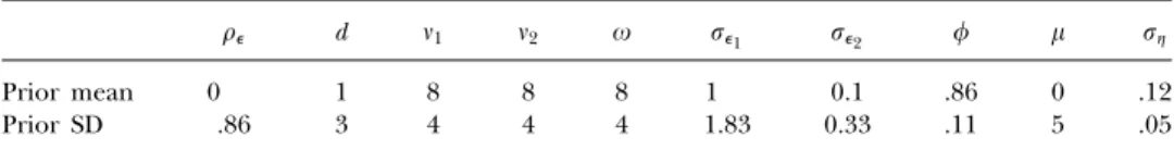
For the last three models, there are two sets of parameters: parameters in the mean equation ( ,d,,1,2), and in the factor equation (,,). We assume that the parameters are mutually independent. The prior distributions are specified as
• ∼U(−1, 1)
• ∗i ∼2
(4), where∗i =i/2,i =1, 2
TABLE 1 Means and standard deviations of prior distributions for parameters in the first six models 11 22 21 1 2 1 2 0 Prior mean 0 8 .86 .86 0 0 0 0 .12 .12 .7 .86 .12 Prior SD .86 4 .11 .11 .33 5 5 .86 .05 .05 3.3 .11 .05 • d ∼N(1, 9) • 2 1 ∼gamma(03, 03) • 2 2 ∼gamma(003, 03) • ∼N(0, 25) • ∗ ∼beta(20, 15), where∗ =(+1)/2 • 2 ∼Inverse-gamma(25, 0025)
We report means and standard errors of these prior distributions for the first six models in Table 1 and those for the last three models in Table 2.
5.3. Results
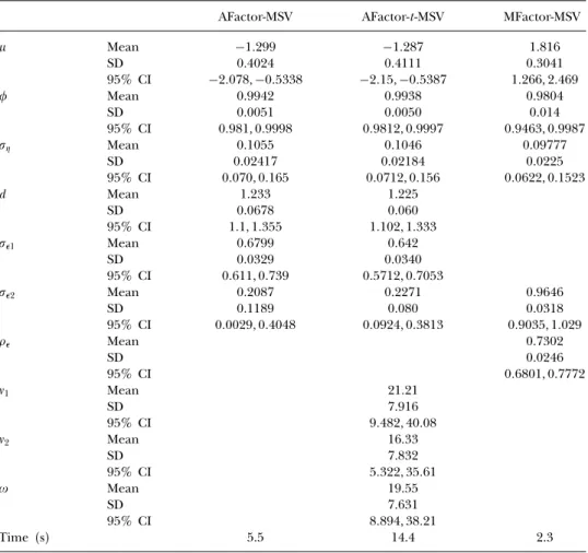
We report means, standard errors, and 95% credible intervals of the posterior distributions for the first six models in Table 3 and those for the last three models in Table 4, as well as the computing time to generate 100 iterations for each of the nine models. The computing time is the central processing unit (CPU) time on a HP XW6000 workstation running WinBUGS1.4. For all models, after a burn-in period of 10,000 iterations and a follow-up period of 100,000, we stored every 20th iteration.
The first thing that can be seen from Tables 3 and 4 is that all nine models can be quickly estimated. The CPU time required for 100 iterations ranges from 2.3 seconds to 14.4 seconds. Moreover, estimating different multivariate SV models in WinBUGS requires little effort in coding, and often no more than a few lines of code have to be changed. Second, the estimated means and standard deviations for the parameters appear quite reasonable and in accordance with estimates documented in the literature. For instance, in Model 1 (MSV), both volatility processes are estimated to be highly persistent. In Model 4 (GCC-MSV), posterior means of both correlation ( and ) are high, as already observed in Harvey et al.
TABLE 2 Means and standard deviations of prior distributions for parameters in the last three models
d 1 2 1 2
Prior mean 0 1 8 8 8 1 0.1 .86 0 .12
TABLE 3 Posterior quantities for parameters in the first six models MSV CC-MSV GC-MSV GCC-MSV DC-MSV t-MSV 1 Mean .0050 .0930 −.1629 −1.094 .0123 .0430 SD .2294 .1263 .2417 2.262 .2001 .1108 95% CI −50,436 −188,319 −689,211 −650, 245 −419,395 −020,242 2 Mean −.710 −.6562 −.4617 −2.454 −.7595 −.5929 SD .4064 .3695 .3725 1.275 .3563 .3873 95% CI −152,026 −136,044 −125,112 −545,−37 −145,−101 −142,040 11 Mean .9770 .9428 .9788 .9764 .9766 .9252 SD .0140 .0418 .0167 .0134 .0135 .0591 95% CI 942,996 838,989 936,998 945,996 944,996 78,986 22 Mean .9920 .9905 .7074 .8622 .9934 .9874 SD .0061 .0089 .1272 .0937 .0052 .0117 95% CI 976,999 966,999 423,920 625,982 980,999 957,999 1 Mean .1107 .0967 .0774 .0807 .0973 .0965 SD .0265 .0220 .0167 .0148 .0198 .0242 95% CI 071,174 061,147 052,116 057,115 066,146 061,153 2 Mean .1044 .0884 .1262 .1431 .0894 .0881 SD .0228 .0203 .0531 .0289 .0187 .0205 95% CI 069,157 059,135 062,269 098,209 061,134 058,138 Mean .7439 .7398 .7325 .7471 SD .0208 .0228 .0202 .0205 95% CI 701,783 692,781 691,770 705,785 12 Mean .4865 SD .2296 95% CI 115, 100 Mean .8363 SD .1240 95% CI 540,988 Mean .1124 SD .031 95% CI 065,189 0 Mean 1.945 SD .2808 95% CI 1387, 2519 Mean .9814 SD .0122 95% CI 950,997 Mean 23.22 SD 7.174 95% CI 1259, 402 Time (s) 3.3 2.7 3.0 9.6 3.5 4.5
(1994). In Model 6 (t-MSV), the posterior mean of is 23.22, suggesting that a heavy-tailed distribution for errors is not needed. In all three factor models, the factor process is estimated to be highly persistent.5 In Model 7 (AFactor-MSV), the factor loading is estimated to be 1.233.
5While the posterior means of are all close to unity and seem to suggest a random walk behavior for ht, we have found that the random walk models give higher DIC values than their stationary counterparts.
TABLE 4 Posterior quantities for parameters in the last three models
AFactor-MSV AFactor-t-MSV MFactor-MSV Mean −1299 −1287 1816 SD 0.4024 0.4111 0.3041 95% CI −2078,−05338 −215,−05387 1266, 2469 Mean 0.9942 0.9938 0.9804 SD 0.0051 0.0050 0.014 95% CI 0981, 09998 09812, 09997 09463, 09987 Mean 0.1055 0.1046 0.09777 SD 0.02417 0.02184 0.0225 95% CI 0070, 0165 00712, 0156 00622, 01523 d Mean 1.233 1.225 SD 0.0678 0.060 95% CI 11, 1355 1102, 1333 1 Mean 0.6799 0.642 SD 0.0329 0.0340 95% CI 0611, 0739 05712, 07053 2 Mean 0.2087 0.2271 0.9646 SD 0.1189 0.080 0.0318 95% CI 00029, 04048 00924, 03813 09035, 1029 Mean 0.7302 SD 0.0246 95% CI 06801, 07772 1 Mean 21.21 SD 7.916 95% CI 9482, 4008 2 Mean 16.33 SD 7.832 95% CI 5322, 3561 Mean 19.55 SD 7.631 95% CI 8894, 3821 Time (s) 5.5 14.4 2.3
Some interesting empirical results can be found from the two new specifications, Model 3 (GC-MSV) and Model 5 (DC-MSV). In Model 3, the posterior mean of 12 is 0.4865 with the lower limit of the 95% posterior credibility interval being greater than zero. It suggests that the volatility in Australian dollar Granger causes the volatility in the New Zealand dollar, consistent with our expectation. As a result of allowing for Granger causality, the posterior mean of the volatility persistence for the New Zealand dollar is reduced from 0.99 to 0.7074. In Model 5 (DC-MSV), the correlation process is reasonably highly persistent, with a posterior mean ofbeing 0.9814. The posterior mean of the long run mean of the time-varying correlation is 0.7195, consistent with what is found in Model 4 (GCC-MSV). All these posterior quantities point toward the importance of time-varying correlation.
TABLE 5 DIC for all models
DIC
Model Value Ranking D pD
MSV 2997.270 9 2958.960 38.320 CC-MSV 2622.090 6 2581.960 40.125 GC-MSV 2616.290 5 2578.890 37.393 GCC-MSV 2608.060 4 2581.110 26.941 DC-MSV 2579.970 3 2524.450 55.523 t-MSV 2624.880 7 2546.940 77.938 AFactor-MSV 2577.750 2 2557.270 20.481 AFactor-t-MSV 2576.560 1 2512.400 64.160 MFactor-MSV 2626.660 8 2599.340 27.326
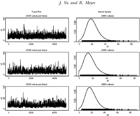
In Table 5 we report DIC together with D and pD for each of the nine models as well as their associated rankings. The best model to describe the bivariate data according to DIC is Model 8 (AFactor-t-MSV), followed closely by Model 7 (AFactor-MSV) and Model 5 (DC-MSV). Figures 2–4 show the trace plots and density functions of the parameters
d,,,,1,2,v1,v2, andin Model 8. The models that have the lowest posterior means of the deviance are Model 5 and Model 8 (AFactor-t-MSV). The models that have the smallest effective numbers of parameters are Model 7 and Model 4 (GCC-MSV). As Model 8, Model 7, and Model 5 all allow for time-varying correlations, the message taken from this model comparison exercise is that correlations do indeed vary over time.
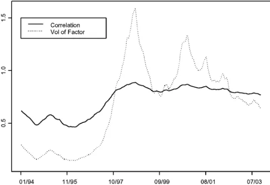
To understand the implications of the better specifications, we obtain smoothed estimates of volatilities and correlations from Model 8 (AFactor-t-MSV) and Model 5 (DC-MSV). In WinBUGS, once the latent processes are sampled and stored, it is trivial to obtain the smoothed estimates of them. We plot the estimates of the two volatilities and the correlations from Model 5 in Figure 5 and the volatilities of the factor and the correlations from Model 8 in Figure 6. Figure 5 reveals that both the Australian dollar and the New Zealand dollar experienced a rapid volatility increase over the period from 1995 to 1998. The smoothed estimate of correlations shown in Figure 5 is interesting. The correlation quickly decreases from 0.75 to 0.45 from the beginning of the sample and reaches the lowest level in 1995. After that, it steadily increases to 0.8 and stays around that level for the
TABLE 6 Geweke’sZ-scores and inefficiency factors for parameters in AFactor-t-MSV
d 1 2 1 2
Z-score −1.485 2.10 −0.835 −0.237 −2.89 1.94 −0.868 −2.92 0.648 IACT 116.78 212.97 84.69 231.61 55.59 90.82 69.62 116.82 107.97
FIGURE 2 Trace plots and density estimates of the marginal distribution ofd,, andin Model 8 (AFactor-t-MSV).
FIGURE 3 Trace plots and density estimates of the marginal distribution of , 1, and 2 in Model 8 (AFactor-t-MSV).
FIGURE 4 Trace plots and density estimates of the marginal distribution of1,2, andin Model 8 (AFactor-t-MSV).
FIGURE 5 Smoothed estimates of volatilities of exchanges rates and time-varying correlations from Model 5 (DC-MSV).
FIGURE 6 Smoothed estimates of volatilities of the factor and time varying correlations from Model 8 (Factor-t-MSV).
rest of sample period. The correlation reaches the peak in 2002, which corresponds to the period of prolonged depreciation of the two currencies against the US dollar. Figure 6 tells a similar story about the volatilities— the volatilities of the common factor have experienced a rapid volatility increase over the period from 1995 to 1998. However, the implication on the correlations is somewhat different. Compared with Figure 5, the correlation in Figure 6 shows more dramatic evidence of nonstationarity in correlations. That is, it seems there is a structural change in the correlation process. The breakdown of the correlation appears to take place at the end of 1998.
As indicated in Section 3, CODA software provides various convergence diagnostics to test if a Markov chain has converged. In this paper we calculate Geweke’sZ-score. To check the simulation inefficiency, following Meyer and Yu (2000), we employ IACT as a measure of inefficiency factor. While more detailed results can be requested from the authors, we choose to report the Z-scores and the inefficiency factors for parameters in Model 8 only in Table 6. It can be seen that, in absolute value, all the
Z-scores are either smaller than the critical values or around them (1.96 is the 5% critical value and 2.56 is the 1% critical value), suggesting that the samplers have converged reasonably well. The inefficiency factor ranges from 55.59 to 212.97, suggesting that the single-move algorithm is not very
efficient and a long sample is needed. When we increase the number of iterations to 500,000, however, the empirical results remain essentially the same.
6. CONCLUSION
In this paper we proposed to estimate and compare multivariate SV models using Bayesian MCMC techniques via WinBUGS. MCMC is a powerful method and has a number of advantages over alternative methods. Unfortunately, writing the first MCMC program for estimating multivariate SV models is not easy, and comparing alternative multivariate SV specifications is computationally costly. WinBUGS imposes a short but sharp learning curve. In the bivariate setting, we show that its implementation is easy and computationally reasonably fast. Also, it is very flexible to handle a rich class of specifications. However, since WinBUGS offers a single-move Gibbs sampling algorithm, as one would expect, we find that the mixing is generally slow and hence a long sample is required. We illustrated the implementation in WinBUGS by exploring and comparing nine bivariate models, including Granger causality in volatilities, time-varying correlations, heavy-tailed error distributions, additive factor structure, and multiplicative factor structure, two of which are new to the SV literature. Our empirical results based on weekly Australian/US dollar and New Zealand/US dollar exchange rates indicate that the models that allow for time-varying coefficients generally fit the data better.
ACKNOWLEDGMENTS
Jun Yu gratefully acknowledges financial support from the Wharton-SMU Research Center and computing support from the Center for Academic Computing, both at Singapore Management University. The research of the second author was supported by the Royal Society of New Zealand Marsden Fund. We also wish to thank two referees for constructive comments, and Manabu Asai, Ching-Fan Chung, Mike McAleer, Yiu Kuen Tse, and seminar participants at the Workshop on Econometric Theory and Applications in Taiwan for helpful discussion.
REFERENCES
Aas, K., Haff, I. (2006). The generalized hyperbolic skew student’st-distribution.Journal of Financial Econometrics4:275–309.
Aguilar, O., West, M. (2000). Bayesian dynamic factor models and portfolio allocation. Journal of Business and Economic Statistics18:338–357.
Akaike, H. (1973). Information theory and an extension of the maximum likelihood principle. In: Proceedings 2nd International Symposium Information Theory. Petrov, B. N., Csaki, F., eds. Budapest: Akademiai Kiado, pp. 267–281.
Andersen, T., Sorensen, B. (1996). GMM estimation of a stochastic volatility model: a Monte Carlo study.Journal of Business and Economic Statistics14:329–352.
Andersen, T., Chung, H., Sorensen, B. (1999). Efficient method of moments estimation of a stochastic volatility model: a Monte Carlo study.Journal of Econometrics91:61–87.
Asai, M., McAleer, M. (2005). The structure of dynamic correlations in multivariate stochastic volatility models.Faculty of Economics. Japan: Saka University.
Asai, M., McAleer, M., Yu, J. (2006). Multivariate stochastic volatility models: a survey. 24(2–3): 443–473.
Bauwens, L., Laurent, S., Rombouts, J. V. K. (2006). Multivariate GARCH: A survey.Journal of Applied Econometrics21:79–109.
Berg, A., Meyer, R., Yu, J. (2004). Deviance information criterion for comparing stochastic volatility models.Journal of Business and Economic Statistics 22:107–120.
Bollerslev, T. (1990). Modelling the coherence in shirt-run nominal exchange rates: a multivariate generalized ARCH approach.Review of Economics and Statistics72:498–505.
Bollerslev, T., Engle, R., Wooldridge, J. M. (1998). A capital asset pricing model with time varying covariances.Journal of Political Economy96:116–131.
Braun, P., Nelson, D., Sunier, A. (1995). Good news, bad news, volatility and betas.Journal of Finance 50:1575–1603.
Chan, D., Kohn, R., Kirby, C. (2005). Multivariate stochastic volatility with leverage. Econometric Reviews 25(2–3):245–274.
Chib, S. (1995). Marginal likelihood from the Gibbs output. Journal of the American Statistical Association90:1313–1321.
Chib, S., Nardari, F., Shephard, N. (2005). Analysis of high dimensional multivariate stochastic volatility models.Journal of Econometrics, forthcoming.
Christodoulakis, G., Satchell, S. E. (2002). Correlated ARCH (CorrARCH): modelling the time-varying conditional correlation between fianacial asset returns.European Journal of Operational Research139:351–370.
Danielsson, J. (1994). Stochastic volatility in asset prices: estimation with simulated maximum likelihood.Journal of Econometrics64:375–400.
Danielsson, J. (1998). Multivariate stochastic volatility models: estimation and comparison with VGARCH models.Journal of Empirical Finance5:155–173.
Diebold, F. X., Nerlove, M. (1989). The dynamics of exchange rate volatility: a multivariate latent-factor ARCH model.Journal of Applied Econometrics 4:1–22.
Ding, Z., Engle, R. (2001). Large scale conditional covariance modelling, estimation and testing. Academia Economic Papers29:157–184.
Durham, G. S. (2005). Monte Carlo methods for estimating, smoothing, and filtering one and two-factor stochastic volatility models.Journal of Econometrics, forthcoming.
Engle, R. (2002). Dynamic conditional correlation—a simple class of multivariate GARCH models. Journal of Business and Economic Statistics17:239–250.
Engle, R., Kroner, K. (1995). Multivariate simultaneous GARCH.Econometric Theory11:122–150. Engle, R., Ng, V., Rothschild, M. (1990). Asset pricing with a factor ARCH covariance structure:
empirical estimates for treasury bills.Journal of Econometrics45:213–237.
Fridman, M., Harris, L. (1998). A maximum likelihood approach for non-Gaussian stochastic volatility models.Journal of Business and Economic Statistics16:284–291.
Gilks, W. (1992). Derivative-free adaptive rejection sampling for Gibbs sampling. In:Bayesian Statistics 4. Bernardo, J. M., Berger, J. O., Dawid, A. P., Smith, A. F. M., eds. Oxford: Oxford University Press, pp. 642–665.
Harvey, A. C. (1990). Forecasting, Structural Time Series Models and the Kalman Filter. New York: Cambridge University Press.
Harvey, A. C., Ruiz, E., Shephard, N. (1994). Multivariate stochastic variance models. Review of Economic Studies61:247–264.
Jacquier, E., Polson, N. G., Rossi, P. E. (1994). Bayesian analysis of stochastic volatility models.Journal of Business and Economic Statistics12:371–389.
Jacquier, E., Polson, N. G., Rossi, P. E. (1995). Priors and models of stochastic volatility models. Unpublished manuscript, University of Chicago.
Jacquier, E., Polson, N. G., Rossi, P. E. (1999). Stochastic volatility: univariate and multivariate extensions. Unpublished manuscript, University of Chicago.
Jungbacker, B., Koopman, S. J. (2006). Monte Carlo likelihood estimation for three multivariate stochastic volatility models.Econometric Reviews25(2–3):385–408.
Kim, S., Shephard, N., Chib, S. (1998). Stochastic volatility: Likelihood inference and comparison with ARCH models.Review of Economic Studies65:361–393.
Knight, J. L., Satchell, S. S., Yu, J. (2002). Estimation of the stochastic volatility model by the empirical characteristic function method. Australian and New Zealand Journal of Statistics
44:319–335.
Lancaster, T. (2004).An Introduction to Modern Bayesian Econometrics. Oxford: Blackwell.
Liesenfeld, R., Richard, J. (2003). Univariate and multivariate stochastic volatility models: estimation and diagnostics. Journal of Empirical Finance10:505–531.
McAleer, M. (2005). Automated inference and learning in modelling financial volatility. Econometric Theory21:232–261.
Melino, A., Turnbull, S. M. (1990). Pricing foreign currency options with stochastic volatility.Journal of Econometrics45:239–265.
Meyer, R., Yu, J. (2000). BUGS for a Bayesian analysis of stochastic volatility models. Econometrics Journal3:198–215.
Meyer, R., Fournier, D. A., Berg, A. (2003). Stochastic volatility: Bayesian computation using automatic differentiation and the extended Kalman filter.Econometrics Journal6:408–420. Neal, R. (1997). Markov chain Monte Carlo methods based on “slicing” the density function.
Technical Report 9722. Department of Statistics, University of Toronto, Canada.
Neal, R. (1998). Suppressing random walks in Markov chain Monte Carlo methods using ordered over-relaxation. In: Learning in Graphical Models. Jordan, M. I., ed. Dordrecht: Kluwer Academic Publishers, pp. 205–230.
Newton, M., Raftery, A. E. (1994). Approximate Bayesian inferences by the weighted likelihood bootstrap.Journal of the Royal Statistical Society, Series B56:3–48 (with discussion).
Pitt, M., Shephard, N. (1999). Time varying covariances: a factor stochastic volatility approach. In: Bernardo, J. M., Berger, J. O., David, A. P., Smith, A. F. M., eds.Bayesian Statistics6. Oxford: Oxford University Press, pp. 547–570.
Quintana, J. M., West, M. (1987). An analysis of international exchange rates using multivariate DLMs.Statistician36:275–281.
Richard, J. F., Zhang, W. (2004). Efficient high-dimensional importance sampling. Working paper, University of Pittsburgh.
Sandmann, G., Koopman, S. J. (1998). Maximum likelihood estimation of stochastic volatility models.
Journal of Econometrics63:289–306.
Selçuk, F. (2004). Free float and stochastic volatility: the experience of a small open economy.
Physica A342:693–700.
Shephard, N. (2005).Stochastic Volatility: Selected Readings. Oxford: Oxford University Press. Spiegelhalter, D. J., Thomas, A., Best, N. G., Gilks, W. R. (1996). BUGS 0.5, Bayesian Inference Using
Gibbs Sampling. Manual (version ii). MRC Biostatistics Unit, Cambridge, UK.
Spiegelhalter, D. J., Best, N. G., Carlin, B. P., van der Linde, A. (2002). Bayesian measures of model complexity and fit (with discussion).Journal of the Royal Statistical Society, Series B64:583–639. Spiegelhalter, D. J., Thomas, A., Best, N. G., Gilks, W. R. (2003).WinBUGS User Manual (Version 1.4).
MRC Biostatistics Unit, Cambridge, UK.
Tsay, R. S. (2002). Analysis of Financial Time Series. New York: John Wiley.
Tse, Y., Tusi, A. (2002). A multivariate GARCH model with time-varying correlations. Journal of Business and Economic Statistics17:351–362.
Yu, J. (2002). Forecasting volatility in the New Zealand stock market. Applied Financial Economics
12:193–202.