SFB
823
Low-frequency estimation of
continuous-time moving
average Lévy processes
Discussion Paper
Denis Belomestny, Vladimir Panov,
Jeannette H. C. Woerner
Low-frequency estimation of continuous-time moving
average Lévy processes
1Denis Belomestnya,b, Vladimir Panovb, Jeannette H. C. Woernerc
aUniversity of Duisburg-Essen, Thea-Leymann-Str. 9, 45127 Essen, Germany bNational Research University Higher School of Economics
Shabolovka, 26, 119049 Moscow, Russia
cTechnische Universität Dortmund, Vogelpothsweg 87, 44227 Dortmund, Germany
Abstract
In this paper we study the problem of statistical inference for a continuous-time moving average Lévy process of the form
Zt =
ˆ
R
K(t−s)dLs, t∈R
with a deterministic kernelKand a Lévy processL. Especially the estimation of the Lévy measure ν of L from low-frequency observations of the process
Z is considered. We construct a consistent estimator, derive its convergence rates and illustrate its performance by a numerical example. On the technical level, the main challenge is to establish a kind of exponential mixing for continuous-time moving average Lévy processes.
Keywords: moving average, Mellin transform, low-frequency estimation
1The study has been funded by the Russian Academic Excellence Project “5-100”.
The first and the third author acknowledge the financial support from the Deutsche Forschungsgemeinschaft through the SFB 823 “Statistical modelling of nonlinear dynamic processes”.
E-mail addresses: [email protected] (D.Belomestny),
1. Introduction
Continuous-time Lévy-driven moving average processes of the form:
Zt=
ˆ ∞ −∞
K(s, t)dLs
with a deterministic kernelKand a Lévy process(Lt)t∈Rbuild a large class of
stochastic processes including semimartingales and non-semimartingales, cf. Basse and Pedersen [1], Basse-O’Connor and Rosinsky [2], Bender, Lindner and Schicks [3], as well as long-memory processes. Starting point was the pa-per by Rajput and Rosinski [4] providing conditions on the interplay between
K and L such that Z is well defined. Continuous-time Lévy-driven moving average processes provide a unifying approach to many popular stochastic models like Lévy driven Ornstein-Uhlenbeck processes, fractional Lévy pro-cesses and CARMA propro-cesses. Furthermore, they are the building blocks of more involved models such as Lévy semistationary processes and ambit pro-cesses, which are popular in turbulence and finance, cf. Barndorff-Nielsen, Benth and Veraart [5].
Statistical inference for Ornstein-Uhlenbeck processes and CARMA cesses is already well-established due to the special structure of the pro-cesses, for an overview see Brockwell and Lindner [6], whereas for general continuous-time Lévy driven moving average processes so far only partial re-sults are known in the literature mainly concerning parameters which enter the kernel function, cf. Cohen and Lindner [7] for an approach via empirical moments or Zhang, Lin and Zhang [8] for a least squares approach. Further results concern limit theorems for the power variation, cf. Glaser [9], Basse-O’Connor, Lachieze-Rey and Podolskij [10], which may be used for statistical inference based on high-frequency data.
In this paper we consider a special case of stationary continuous-time Lévy-driven moving average processes of the form Zt =
´∞
−∞K(s −t)dLs
and aim to infer the unknown parameters of the driving Lévy process from its low-frequency observations. Our setting especially includes the case of Gamma-kernels of the form K(t) =tαe−λt1[0,∞)(t)withλ >0andα >−1/2,
which serve as a popular kernel for applications in finance and turbulence, cf. Barndorff-Nielsen and Schmiegel [11]. The special symmetric case of the well-balanced Ornstein-Uhlenbeck process has been discussed in Schnurr and Woerner [12].
In fact, the resulting statistical problem is rather challenging for several reasons. On the one hand, the set of parameters, i.e., the so-called Lévy-triplet of the driving Lévy process contains, in general, an infinite dimen-sional object, a Lévy measure making the statistical problem nonparametric. On the other hand, the relation between the parameters of the underlying Lévy process (Lt) and those of the resulting moving average process (Zt) is
rather nonlinear and implicit, pointing out to a nonlinear ill-posed statistical problem. It turns out that in Fourier domain this relation becomes exponen-tially linear and has a form of multiplicative convolution. This observation underlies our estimation procedure, which basically consists of three steps. First, we estimate the marginal characteristic function of the Lévy-driven moving average process (Zt). Then we estimate the Mellin transform of the
second derivative of the log-transform of the characteristic function. Finally, an inverse Mellin transform technique is used to reconstruct the Lévy density of the underlying Lévy process.
The paper is organized as follows. In the next session, we explain our setup and discuss the correctness of our model. In Section 3, we present the estimation procedure. Our main theoretical results related to the rates of convergence of the estimates are given in Section 4. Next, in Section 5, we provide a numerical example, which shows the performance of our procedure. All proofs are collected in the appendix.
2. Setup
In this paper we study a stationary continuous-time moving average (MA) Lévy process (Zt)t∈R of the form:
Zt=
ˆ ∞ −∞
K(t−s)dLs, t ∈R, (1)
where K:R→R+ is a measurable function and(Lt)t∈R is a two-sided Lévy
process with the triplet T = (γ, σ2, ν). As shown in [4], under the conditions
ˆ R ˆ R\{0} |K(s)x|2 ∧1ν(dx)ds <∞, (2) σ2 ˆ R K2(s)ds <∞, (3) ˆ R K(s) γ+ ˆ R x 1{|xK(s)|≤1}−1{|x|≤1} ν(dx) ds <∞ (4)
the stochastic integral in (1) exists. In what follows, we assume that K ∈
L1(R)∩L2(R)and the Lévy measure ν satisfies
ˆ
x2ν(dx)<∞, (5)
that is, the Lévy process L has finite second moment. In fact, (3) is trivial in this case; condition (2) directly follows from the inequality
ˆ R ˆ R\{0} |K(s)x|2∧1 ν(dx)ds ≤ ˆ R ˆ R\{0} |K(s)x|2ν(dx)ds = ˆ R (K(s))2ds· ˆ R\{0} x2ν(dx)ds.
As to the condition (4), we have
ˆ R K(s) γ− ˆ R x1{|x|≤1}ν(dx) + ˆ R xK(s)1{|xK(s)|≤1}ν(dx) ds = ˆ R K(s)E[L1]− ˆ R xK(s)1{|xK(s)|>1}ν(dx) ds ≤ |E[L1]| ˆ R K(s)ds+ ˆ R ˆ R x2(K(s))2ν(dx)ds.
In the sequel we assume that K ∈L1(R)∩L2(R)and
ˆ
x2ν(dx)<∞. (6)
Moreover, under the above assumptions, the process (Zt)t∈R is strictly
sta-tionary with the characteristic function of the form
Φ(u) :=EeiuZt= exp (ψ(u)), (7) where Ψ(u) := ˆ R ψ(uK(s))ds and ψ(u) :=iuγ−σ2u2/2 + ˆ R eiux−1−iux1{|x|≤1} ν(dx).
Our main goal is the estimation of the parameters of the Lévy process L
from low-frequency observations of the process Z given that the function K
3. Mellin transform approach
3.1. Main idea
Let L be a Lévy process with the Lévy triplet (µ, σ2, ν), where ν is an absolutely continuous w.r.t. to the Lebesgue measure on R+ and satisfies
(6). Denote by ν(x) the density ofν and setν(x) :=x2ν(x).For the sake of
clarity we first assume that σ is known and ν is supported onR+,i.e. Lis a
sum of a Brownian motion and subordinator. Set
Ψσ(u) := Ψ(u) + σ2u2 2 ˆ R K2(x)dx. It follows then Ψ00σ(u) = ˆ R ψ00(uK(x))· K2(x)dx=− ˆ R F[ν] (uK(x))· K2(x)dx,
where F[ν] stands for the Fourier transform of ν. Next, let us compute the Mellin transform of Ψ00σ: M[Ψ00σ] (z) = − ˆ R+ ˆ R F[ν] (uK(x))· K2(x)dx uz−1du = − ˆ R ˆ R+ F[ν] (uK(x) )·uz−1du K2(x)dx = −M[F[ν]](z)· ˆ R (K(x))2−zdx , (8)
for allz such that´
R(K(x)) 2−Re(z)dx <∞and ´ R+|F[ν] (v)| ·v Re(z)−1dv <∞. Since ν ∈L1(R+), it holds M[F[ν]](z) = ˆ ∞ 0 vz−1 ˆ ∞ 0 eixvν(x)dx dv = M ei·(z)· M ν(1−z).
Note that the Mellin transform M
ν
(1−z)is defined for all z withRe(z)∈
(0,1), provided ν is bounded at 0. Next, using the fact that
M[ei·](z) = Γ(z) [cos(πz/2) +isin(πz/2)] = Γ(z)eiπz/2
for all z with Re(z)∈(0,1)(see [13], 5.1-5.2), we get
where
Q(z) :=−Γ(z)eiπz/2
ˆ
R
(K(x))2−zdx. (9) Finally, we apply the inverse Mellin transform to get
ν(x) = 1 2πi ˆ c+i∞ c−i∞ M[ν](z)x−zdz = 1 2πi ˆ c+i∞ c−i∞ M[Ψ00σ](1−z) Q(1−z) x −z dz (10)
for c ∈ (0,1). The formula (10) connects the weighted Levy density ν to the characteristic exponent Ψσ of the process Z and forms the basis for our
estimation procedure.
Remark 1. If σ2 is supposed to be unknown, one can estimate it by not-ing that for a properly chosen bounded kernel w with supp(w) ⊆ [1,2] and
´∞ 0 w(u)du= 1, ˆ R+ wn(u)Ψ00(u)du = −σ2 ˆ R K2(x)dx − ˆ R ˆ R+ wn(u)F[ν] (uK(x))K2(x)du dx = −σ2 ˆ R K2(x)dx − ˆ R ˆ R+ w(u)F[ν] (uUnK(x))K2(x)du dx
with wn(u) := Un−1w(u/Un) and some sequence Un → ∞. Suppose that
|F[ν](u)| ≤ C(1 +u)−α for all u ≥ 0 and some constants α > 0, C > 0,
then ˆ R ˆ R+ w(u)F[ν] (uUnK(x))K2(x)du dx ≤ kwk∞ ˆ R K2(x) (1 +UnK(x))α dx→0
as n→ ∞.For example, in the case of a one-sided exponential kernelK(x) =
e−xII(x≥0), we derive ˆ R K2(x) (1 +UnK(x))α dx= 1 U−2 n ˆ Un 0 z (1 +z)α dz . Un−α, α <2, Un−2log(Un), α = 2, Un−2, α >2, as n→ ∞.
Remark 2. Let us remark on the general case where the jump part of L is not necessary a subordinator. In this case one can show that
M[Ψ00σ(−·)] (u) +M[Ψ00σ(·)] (u) 2 = − M ν+ (1−z) +M ν− (1−z) ·cosπz 2 Γ(z)· ˆ R (K(x))2−zdx and M[Ψ00σ(·)] (u)− M[Ψ00σ(−·)] (u) 2i = − M ν+ (1−z)− M ν− (1−z) ·sinπz 2 Γ(z)· ˆ R (K(x))2−zdx,
where ν+(x) = ν(x)·1(x≥0) andν−(x) = ν(−x)·1(x≥0).Using the above
formulas, one can express M
ν− , M ν+ in terms of M[Ψ00σ(−·)], M ν−
and apply the Mellin inversion formula to reconstruct ν− and ν+.
3.2. Estimation procedure
Assume that the process Z is observed on the equidistant time grid
{∆,2∆, . . . , n∆}. Our aim is to estimate the Lévy density ν of the process
L. First we approximate the Mellin transform of the function
Ψ00σ(u) = Φ 00(u) Φ(u) − Φ0(u) Φ(u) 2 +σ2kKk2 L2 via Mn[Ψ00σ](1−z) := ˆ Un 0 " Φ00n(u) Φn(u) − Φ0n(u) Φn(u) 2 +σ2kKk2L2 # u−zdu, (11) where Φn(u) := 1 n n X k=1 exp{iZk∆u}
and a sequence Un → ∞ as n → ∞. Second, by regularising the inverse
Mellin transform, we define
νn(x) := 1 2πi ˆ c+iVn c−iVn Mn[Ψ00σ](1−z) Q(1−z) x −z dz (12)
for some c ∈ (0,1) and some sequence Vn → ∞, which will be specified
later. In the next section we study the properties of the estimate νn(x). In
particular, we show thatνn(x)converges toν(x)and derive the corresponding
convergence rates.
4. Convergence
Assume that the following conditions hold.
(AN) For some A > 0 and α ∈ (0,1), γ >0, c ∈(0,1) the Lévy density ν
fulfills ˆ R (1 +|y|)α|F[ν](y)|dy ≤A, (13) ˆ R eγ|u||M[ν](c+iu)|du≤A, (14) ˆ R+ (x∨x2)ν(x)dx ≤A. (15)
Theorem 1. Suppose that (AN) holds, K is a nonnegative kernel with K ∈
L1(R)∩L2(R). Denote Dj(u) := (Φ
(j)
n (u)−Φ(j)(u))/Φ(u), j = 0,1,2, . . . Let
for any real valued function f onR, kfkU
n := supu∈[−Un,Un]|f(u)|. Fix some
K >0 and denote AK := max j=0,1,2kDjkUn ≥Kεn , K ≥0.
Let εn, Un be two sequences of positive numbers such that εn → 0, Un → ∞
as n→ ∞, and moreover
Kεn 1 +kΨ0σkUn
ChoosingεnandUnin such a way is always possible, sinceΨ0σ(0) =ψ
0(0)´ K(s)ds
is finite. Then on the set AK the estimateνn(x) given by (12) with the same
c∈(0,1) as in (14) satisfies sup x∈R+ {xc|νn(x)−ν(x)|} ≤ 1 2π ˆ {|v|≤Vn} Ωn |Q(1−c−iv)|dv+ A 2πe −γVn,
where Q as in (9), Vn is a sequence of positive numbers and
Ωn= 2KεnUn1−c 2 +kΨ00σkU n+kΨ 0 σk 2 Un + 3kΨ 0 σkUn + A+ 2 αA 1−c ˆ R K(x)c+1 1 +UnK(x) −α dx. Remark 3. Note that in case of supp(ν) ⊆ R+, the sum 2 + kΨ00σkUn +
kΨ0σk2U
n+ 3kΨ
0
σkUn can be uniformly bounded. Indeed,
ψ0(u)−σ2u = iµ+ ˆ R+ ixeiuxν(x)dx≤µ+ ˆ R+ xν(x)dx≤µ+A, by (15). Analogously, ψ00(u)−σ2 = ˆ R+ x2eiuxν(x)dx ≤ ˆ R+ x2ν(x)dx≤A. Therefore Ψ0σ Un = ˆ R (ψ0(uK(x))−σ2u)K(x)dx Un ≤(µ+A)kKkL1, Ψ00σ Un = ˆ R (ψ00(uK(x))−σ2)K2(x)dx Un ≤AkKk2 L2,
where the integrals in the right-hand sides are bounded due to the assumption
K ∈L1(
R)∩L2(R).
Example 1. Consider a tempered stable Lévy process (Lt) with
ν(x) =x−η−1·e−λx, x≥0, η ∈(0,1), λ >0. (16)
Since
we derive that (14)holds for all0< γ < π/2andα >0due to the asymptotic properties of the Gamma function. Furthermore,
F[ν](u) = (iu−λ)−(2−η)Γ(2−η)
and hence (13) holds for any 0< α <2−η. Moreover, ν satisfies (15).
Let us now estimate the probability of the eventAK.The following result
holds.
Theorem 2. Suppose that the following assumptions are fulfilled.
1. The kernel K satisfies
∞ X j=−∞ F[K] 2π j ∆ ≤K∗ (17) and (K?K)(∆j)≤κ0 |j|κ1e−κ2|j|, ∀j ∈Z (18)
for some positive constantsK∗,κ0, κ1 andκ2,such that the all
eigenval-ues of the matrix ((K?K)(∆(j−k))k,j∈Z are bounded from below and
above by two finite positive constants.
2. The Lévy measure ν satisfies
ˆ
|x|>1
eRxν(dx)≤AR
for some R >0 and AR >0.
Then under the choice
εn= r log(n) n ·exp C1σ2Un2 ˆ (K(x))2dx
with C1 =A/2, it holds for anyK >0
P AK ≤ √C2 K √ Unn(1/4)−C3K 2 log1/4(n) ,
where the positive constants C1, C2 may depend on K∗, AR and κi, i = 1,2.
Hence by an appropriate choice of K we can ensure that P(AK) → 0 as
Example 2. Consider the class of symmetric kernels of the form
K(x) = |x|re−ρ|x|
, (19)
where r is a nonnegative integer and ρ >0. Let us check the assumptions of Theorem 2. We have F[K](u) = Γ(r+ 1) 1 (iu−ρ)r+1 + 1 (−iu−ρ)r+1
and (17) holds. Assumption (18) is proved in Lemma 2.
Corollary 1. Consider again a class of kernels of the form
K(x) = |x|re−ρ|x|
,
whereris a nonnegative integer andρ >0,and assume that the Lévy measure
ν satisfies the set of assumptions (AN). Then
Ωn .KεnUn1−c+U −α n , n→ ∞ and ˆ {|v|≤Vn} 1 |Q(1−c−iv)|dv . ( Vnc+3/2, r = 0, Vc+1 n , r ≥1. As a result we have on AK sup x∈R+ {xc|νn(x)−ν(x)|}.Vnζ εnUn(1−c)+U −α n +e−γVn
with ζ =c+ 1 +II{r = 0}/2. By taking Vn =κlog(Un) with κ > α/γ and
Un =θlog1/2(n) for any θ < A
´ (K(x))2dx−1/2, sup x∈R+ {xc|νn(x)−ν(x)|}.log−α/2(n), n→ ∞. 4.1. Discussion
The proof of Theorem 2 is based on some kind of exponential mixing for the general Lévy-driven moving average processes of the form (1). In fact, such mixing properties were established in the literature only for the processesZcorresponding to the exponential kernel functionK,see, e.g. [14]. The assumption of Theorem 2 may seem to be strong, but as shown above, are fulfilled for the family of kernels (19).
5. Numerical example
5.1. Simulation.
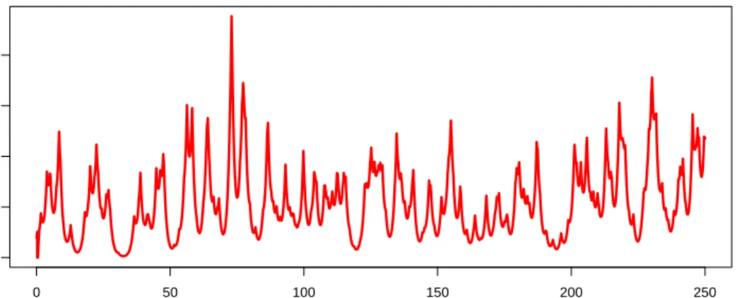
Consider the integral Zt :=
´
RK(t−s)dLs with the kernel K(x) = e
−|x|
and the Lévy process
Lt=L
(1)
t II{t >0} −L (2)
−tII{t <0},
constructed from the independent compound Poisson processes
L(1)t =d L(2)t =d
Nt
X
k=1 ξk,
where Ntis a Poisson process with intensity λ, andξ1, ξ2, ...are independent
r.v.’s with standard exponential distribution. Note that the Lévy density of the process L(1)t is ν(x) =λe−x.
Fork = 1,2, denote the jump times of L(tk) by s(1k), s(2k), ... and the corre-sponding jump sizes by ξ(1k), ξ(2k), ...Then
Zt= ∞ X j=0 K(t−s(1)j )ξj(1)− ∞ X j=0 K(t+s(2)j )ξj(2).
In practice, we truncate both series in the last representation by finding a value xmax:= maxx∈R+{K(x)> α} for a given level α. Let
˜ Zt = X k∈K(1) K(t−s(1)j )ξj(1)− X k∈K(2) K(t+s(2)j )ξj(2), where K(1) := nk : max(0, t−xmax)< s (1) k < t+xmax o , K(2) := n k : 0< s(2)k <max(0,−t+xmax) o .
For simulation study, we take λ= 1, α= 0.01 (and thereforexmax = 6.908).
0 50 100 150 200 250 0 2 4 6 8 t Zt
Figure 1: Typical trajectory of the process Zt constructed from the compound Poisson
process with positive jumps.
5.2. General idea of the estimation procedure.
In practice the estimation procedure described in Section 3.1 can be slightly simplified under the assumption that the Lèvy process L has no drift. In this case, one can consider the first derivative of the functionΨσ(u)
instead of the second, and get that
M[Ψ0σ](z) =Qe(z)· M[ν](1−z), Re(z)∈(0,1), where e Q(z) =iΓ(z) exp{iπz/2} ˆ R (K(x))1−zdx.
The estimation scheme mainly follows the original idea: we first estimate the Mellin transform of the function Ψ0σ, and then infer on the Lévy measure ν
by applying the Mellin transform techniques. Below we describe these steps in more details.
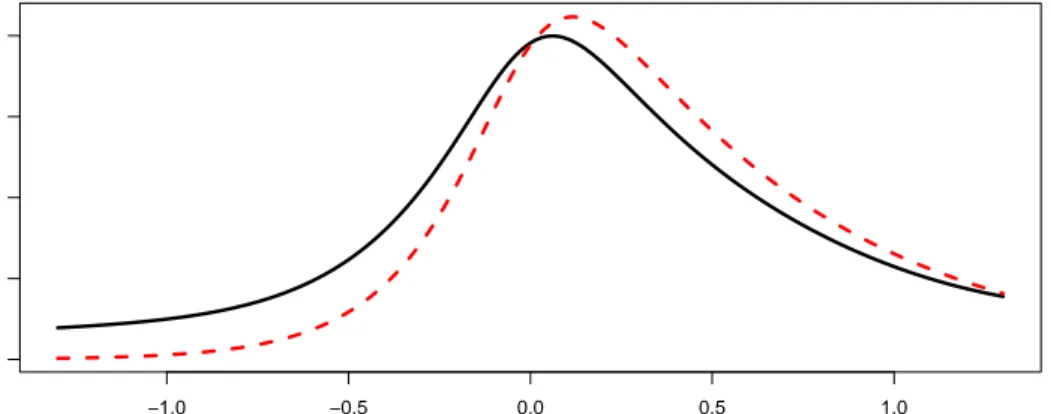
Estimation of the Mellin transform of Ψ0(·). The most natural estimate is Mn[Ψ0](1−z) := i ˆ Un 0 mean(Zk∆eiuZk∆) mean(eiuZk∆) u −z du. (20)
−1.0 −0.5 0.0 0.5 1.0 0 2 4 6 8 v abs(Mel)
Figure 2: Absolute values of the empirical (black solid) and theoretical (red dashed) Mellin transforms of the functionΨ0(·)depending on the imaginary part of the argument.
In order to improve the numerical rates of convergence of the integral involved in (20), we slightly modify this estimate:
Mn[Ψ0](1−z) := i ˆ Un 0 hmean(Zk∆eiuZk∆) mean(eiuZk∆) −mean(Z)e iuiu−z du + 2iλΓ(1−z) exp{iπ(1−z)/2}.
Note that Mn[Ψ0](1−z)is also a consistent estimate of M[Ψ0](1−z)(since
mean(Z)→2λ), but involves the integral with better convergence properties. In our case M[ν](z) =λΓ(1 +z), and therefore the Mellin transform of the function Ψ0 is equal to
M[Ψ0](1−z) =Qe(1−z)· M[ν](z) = 2iλ
Γ(1−z)Γ(1 +z)
z e
iπ(1−z)/2.
We estimate M[Ψ0](1 −z) for z = c+ivk, where c is fixed and vk, k =
1, . . . , K, are taken on the equidistant grid from (−Vn) to Vn with step δ =
2Vn/K. Typical behavior of the the Mellin transform M[Ψ0](1−z) and its
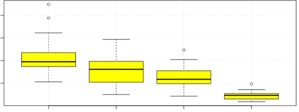
● ● ● ● 1000 5000 10000 20000 0.005 0.010 0.015 0.020 ν n
Figure 3: Boxplot of the estimateR(˜νn?)based on 20 simulation runs.
Estimation of ν(x). Finally, we estimate the Lévy density ν(x) by
˜ νn(x) := δ 2πx K X k=1 Re ( Mn[Ψ0](1−c−ivk) e Q(1−c−iv) ·x −(c+ivk) )
and measure the quality of this estimate by the L2-norm on the interval
[1,3] : R(˜νn) = ˆ 3 1 (˜νn(x)−ν(x)) 2 dx.
To show the convergence of this estimate, we made simulations with different values of n. The parametersUn andVnare chosen by numerical optimization
of R(˜νn). The results of this optimization, for different values of n, as well
as the means and variances of the estimate ν˜n based on 20 simulation runs,
are given in the next table.
n Un Vn mean (R(˜νn)) Var (R(˜νn))
1000 0.4 1.1 0.0109 1.62∗10−5
5000 0.4 1.2 0.0079 9.07∗10−6
10000 0.5 1.3 0.0063 6.56∗10−6
The boxplots of this estimate based on 20 simulation runs are presented on Figure 3.
Appendix A. Proof of Theorem 1
Denote Gj(u) = Ψ (j) σ,n(u)−Ψσ(j)(u), j = 1,2,where Ψσ,n(u) = log Φn(u) + σ2u2 2 ˆ R K2(x)dx. Then G1(u) = D1(u)−D0(u)Ψ0σ(u) 1 +D0(u) , (A.1) G2(u) = Ψ00σ(u) + (Ψ0σ(u))2 + Ψ0σ(u)G1(u) D0(u) 1 +D0(u) −(2Ψ 0 σ(u) +G1(u))D1(u) 1 +D0(u) + D2(u) 1 +D0(u) . (A.2) We have νn(x)−ν(x) = 1 2πi ˆ c+iVn c−iVn Mn[Ψ00σ](1−z)− M[Ψ00σ](1−z) Q(1−z) x−zdz − 1 2πx ˆ {|v|≥Vn} M[ν](c+iv)x−(c+iv)dv and xc(νn(x)−ν(x)) = 1 2π ˆ {|v|≤Vn} R1(v) +R2(v) Q(1−c−iv)x −ivdv − 1 2π ˆ {|v|≥Vn} M[ν](c+iv)x−ivdv, (A.3) where R1(v) := ˆ Un 0 G2(u)u−c−ivdu and R2(v) :=− ˆ ∞ Un Ψ00σ(u)u−c−ivdu.
We have on AK, under the assumption Kεn(1 +kΨσ0kUn) ≤ 1/2, that the
denominator of the fractions in G1 and G2 can be lower bounded as follows:
min u∈[−Un,Un] |1 +D0(u)| ≥1− max u∈[−Un,Un] |D0(u)| ≥1−Kεn≥1/2. Therefore, kG1kUn ≤ 2Kεn 1 +kΨ0σkUn ≤1 kG2kUn ≤ 2Kεn 1 +kΨ00σkU n+ (Ψ0σ)2 Un + (1 +kΨ0σkU n)kG1kUn+ 2kΨ 0 σkUn , Thus |R1(v)| ≤2KUn1−cεn 2 +kΨ00σkU n+kΨ 0 σk 2 Un + 3kΨ 0 σkUn . Since Ψ00σ(u) = − ˆ ∞ ∞ K2(x)· F[ν](uK(x))dx,
it holds for any z ∈C
ˆ ∞ Un Ψ00σ(u)u−zdy = − ˆ ∞ −∞ K2(x) ˆ ∞ Un F[ν](uK(x))u−zdu dx = − ˆ ∞ −∞ [K(x)]z+1 ˆ ∞ UnK(x) F[ν](v)v−zdv dx.
Next, for any fixed x ∈ R, we can upper bound the inner integral in the right-hand side of the last formula:
ˆ ∞ UnK(x) F[ν](v)v−zdv ≤(1 +UnK(x)) −α · ˆ ∞ 0 v−Re(z)(1 +v)α|F[ν](v)| dv.
Due to (13) we get that for any z with Re(z)∈(0,1) it holds
ˆ ∞ 0 v−Re(z)(1 +v)α|F[ν](v)| dv < ¯ δ 1−Re(z) +A
with δ¯= 2α´
R+x
2ν(x)dx ≤2αA due to (15). Finally, we conclude that
|R2(v)|:= ˆ ∞ Un Ψ00σ(y)y−c−ivdy ≤ ¯ δ 1−c +A × ˆ R [K(x)]c+1(1 +UnK(x)) −α dx.
Now an upper bound for the last term in (A.3) follows from the assumption on the Mellin transform of the function ν¯. Indeed, since (14) is assumed, it holds ˆ {|u|≥Vn} M[ν](c+iu)x−iudu ≤e−γVn ˆ {|u|≥Vn} eγVn|M[ν](c+iu)| du≤Ae−γVn.
This observation completes the proof.
Appendix B. Proof of Corollary 1
For the sake of simplicity we consider the caseρ= 1.We divide the proof into several steps. For the sake of simplicity we assume that either the kernel
Kis symmetric or is supported onR+,so that it suffices to study the integral
over R+.
1. Upper bound for Λn:=
´
R+
K(x)c+11 +UnK(x)
−α
dx. Note that the function K(x) = xre−x has two intervals of monotonicity on
R+: [0, r] and
and g2 : [0, rre−r]→[r,∞). Then Λn = ˆ r 0 + ˆ ∞ r [K(x)]c+1[1 +UnK(x)] −α dx = ˆ rre−r 0 wc+1(1 +Unw) −α g01(w)dw + ˆ 0 rre−r wc+1(1 +Unw) −α g20(w)dw = ˆ rre−r 0 wc+1(1 +Unw) −α G(w)dw = Un−c−2 ˆ 1 0 + ˆ rre−rU n 1 ! yc+1(1 +y)−α·G(y/Un)dy =:J1+J2,
where G(·) = g01(·)−g20(·). In what follows, we separately analyze the sum-mands J1 and J2.
1a. Upper bound for J1.. Clearly, the behavior of the function G(·) at
zero is crucial for the analysis ofJ1. SinceK(g1(y)) =yfor anyy∈[0, rre−r],
we get g1(0) = 0 and moreover as y→0,
g01(y) = 1 K0(g 1(y)) = 1 [g1(y)]r−1e−g1(y)(r−g1(y)) 1 r[g1(y)]r−1 .
Analogously, due to K(g2(y)) = y for any y ∈ [0, rre−r], we conclude that
limy→0g2(y) = +∞, and asy→0
g02(y) = 1 [g2(y)]r−1e−g2(y)(r−g2(y)) −1 [g2(y)]re−g2(y) = −1 K(g2(y)) = −1 y .
For further analysis of the asymptotic behaviour of g1(·) we apply the
asymptotic iteration method. We are interested in the behaviour of the solution g1(y) of the equation
asy→0. Note that the distinction between the solutions is in the asymptotic behaviour as y → 0: g1(y) → 0, g2(y) → ∞. Let us iteratively apply the
recursion ϕn+1 =ϕn− f(ϕn) f0(ϕ n) =ϕn− ϕrne−ϕn −y ϕr−1 n e−ϕn(r−ϕn) , n= 1,2, ...
Motivated by the power series expansion of the function e−x at zero,
xre−x =xr−xr+1+ 1
2x
r+2+o(xr+2),
we take for the initial approximation of g1(y), the function ϕ0 =y1/r. Then
ϕ1(y) = y1/r− ye−y1/r −y y(r−1)/re−y1/r (r−y1/r) = y1/r 1− e −y1/r −1 e−y1/r (r−y1/r) ! = y1/r+O(y2/r).
Finally, we conclude that as y→0,
G(y) = 1 ry(r−1)/r (1 +o(1)) + 1 y(1 +o(1)) = 1 y(1 +o(1)).
Therefore J1 can be upper bounded as follows:
J1 ≤ C3Un−c−1
ˆ 1 0
yc(1 +y)−α(1 +o(1)) dy.
The integral in the right-hand side converges iff ´01ycdy < ∞. Since c ∈
(0,1), we get J1 .Un−c−1.
1b. Asymptotic behaviour of J2. Analogously, the asymptotic behavior
of J2 crucially depends on the behavior of G(y)at the pointy=rre−r. Note
that as y→rre−r, g0k(y) = 1 K0(g k(y)) = 1 [gk(y)]r−1e−gk(y)(r−gk(y)) C r−gk(y)
for k = 1,2. Taking logarithms of both parts of the equation xre−x =y and
changing the variablesu=x−rand δ=rre−r−y,we arrive at the equality
u=rlog1 + u r −log 1− δ rre−r .
Consider this equality as u→0 and δ→0+,we get
u=r u r − 1 2 u2 r2 + δ rre−r +O δ 2 +O(u3), and therefore u=±√2r1−rer·√δ+O(δ) +O(u3/2)
corresponding to the functions g1 and g2. Finally, we conclude
|G(y)| C √ 2 √ r1−rer 1 √ rre−r−y, y→r r e−r, and therefore J2 ∼ Un−c−3/2 ˆ rre−rU n 1 yc+1(1 +y)−α· √ 1 rre−rU n−y dy.
We change the variable in the last integral:
z = s rre−rU n−1 rre−rU n−y , y=rre−rUn+ 1−rre−rU n z2 ,
and get with Uen=rre−rUn
J2 Un−c−3/2 ˆ ∞ 1 e Un+ 1−Uen z2 !c+1 · 1 +Uen+ 1−Uen z2 !−α ·q z e Un−1 2(Uen−1) z3 dz. Therefore, J2 C4Un−c−3/2Uenc+1 e Un+ 1 −αq e Un−1, n → ∞,
with some constant C4 > 0 and we conclude that J2 C5Un−α as n → ∞.
To sum up, Λn.U
−min(α,c+1)
2. Upper bound for Hn:= ´ {|v|≤Vn}|Q(1−c−iv)| −1 dv. Recall that Hn= ˆ {|v|≤Vn} e−πv/2 Γ(1−c−iv) · ´ R(K(x)) c+1+iv dx dv
Note that for our choice of the functionK(·), it holds for any z ∈C
ˆ R (K(x))zdx= 2 ˆ R+ (xre−x)zdx= 2 lim R→+∞ ˆ γR(z) urze−udu ·z−(rz+1),
where γR(z) is the part of the complex line {(xRe(z), xIm(z)), x∈[0, R]}.
Note that due to the Cauchy theorem, for any z with positive real part
ˆ R+ urze−ρudu= lim R→+∞ ˆ γR(z) urze−udu+ lim R→+∞ ˆ cR urze−udu (B.1) with cR := {(Rcos(θ), Rsin(θ)), θ ∈(0,arctan(Im(z)/Re(z))}. Since the
last limit in (B.1) is equal to 0, we conclude that
ˆ
R
(K(x))c+1+ivdx= 2 Γr(c+ 1) + 1 +ivr·e−(r(c+1)+1+ivr)·log(c+1+iv).
Next, using the fact that there exists a constantC >¯ 0such that|Γ(α+iβ)| ≥
¯
C|β|α−1/2e−|β|π/2 for any α ≥ −2,|β| ≥ 2 (see Corollary 7.3 from [15]), we
get that e−πv/2 |Γ(1−c−iv)| ≤v c−1/2, and moreover ˆ R (K(x))c+1+ivdx = 2 |Γ(r(c+ 1) + 1 +ivr)| ((c+ 1)2+v2)(r(c+1)+1)/2e−vrarctan(v/(c+1)).
The asymptotic behavior of the last expression depends on the valuer. More precisely, ˆ R (K(x))c+1+ivdx ∼ 2 c(vr)r(c+1)+1/2e−vrπ/2 ((c+1)2+v2)(r(c+1)+1)/2 e−vrarctan(v/(c+1)) ∼v −1/2, if r = 1,2, ..., v−1, if r= 0.
as v → +∞. Finally, we conclude that Hn . Vnc+1, if r = 1,2, ..., and
Hn.V
c+3/2
Appendix C. Mixing properties of the Lévy-based MA processes Theorem 3. Let (Lt) be a Lévy process with Lévy triplet (µ, σ2, ν), where
σ > 0 and supp(ν)⊆ R+. Consider a Lévy-based moving average process of
the form
Zs =
ˆ
K(s−t)dLt, s ≥0
with a nonegative kernel K. Fix some ∆>0 and denote
ZS := (Zj∆)j∈S
for any subset S of {1, . . . , n}. Fix two natural numbers m and p such that
m+p ≤n. For any subsets S ⊆ {1, . . . , m} and S0 ⊆ {p+m, . . . , n}, let g
and g0 be two real valued functions on R|S| and R|S0| satisfying
maxn e −R> S·g L1, e −R> S0·g0 L1 o <∞
for someRS ∈R|S|+ andRS0 ∈R|S 0| + ,and denoteC◦ := e −R> S·g L1· e −R> S0·g0 L1.
Suppose that the Fourier transform Kb of K fulfils
K∗ := ∞ X j=−∞ b K 2πj ∆ <∞ and ˆ |x|>1 eR∗xx2ν(dx)≤AR∗ for R∗ = kRS∪S0k∞K∗ ∆ . Then |Cov (g(ZS), g0(ZS0))| ≤ CRC◦max |l|>p (K?K) (l∆) (C.1) × ˆ kuS∪S0 −iRS∪S0k2exp −σ2λS∪S0(u)duS∪S0, where λS(u) := P
k,j∈Sukuj(K?K)(∆(k− j)) for any u ∈ Rn and CR =
exp(σ2λ
Proof. We have for any S ⊆ {1, . . . , n} ΦS(uS −iRS) := E " exp iX j∈S ujZj∆+ X j∈S RjZj∆ !# = exp ˆ ψ X j∈S (uj −iRj)K(t−j∆) ! dt ! ,
where uS := (uj ∈R, j ∈S)and RS := (Rj ∈R+, j ∈S),provided
E " exp X j∈S RjZj∆ !# <∞.
Denote for any subsets S ⊆ {1, . . . , m} and S0 ⊆ {p+m, . . . , n},
D(uS−iRS, uS0 −iRS0)
:= ΦS,S0(uS−iRS, uS0−iRS0)−ΦS(uS−iRS)ΦS0(uS0 −iRS0),
where it is assumed that
E " exp X j∈S∪S0 RjZj∆ !# <∞
Then using the elementary inequality |ez−ey| ≤ (|ez| ∨ |ey|)|y−z|, y, z ∈
C, we derive |D(uS−iRS, uS0 −iRS0)| ≤ {|ΦS,S0(uS −iRS, uS0 −iRS0)| ∨ |ΦS(uS−iRS)ΦS0(uS0 −iRS0)|} × ˆ ( ψ X j∈S∪S0 (uj −iRj)K(x−j∆) ! −ψ X j∈S (uj−iRj)K(x−j∆) ! −ψ X j∈S0 (uj −iRj)K(x−j∆) !) dx .
Due to Lemma 1 and the Poisson summation formula, we derive |D(uS−iRS, uS0 −iRS0)| ≤ {|ΦS,S0(uS −iRS, uS0 −iRS0)| ∨ |ΦS(uS−iRS)ΦS0(uS0 −iRS0)|} × " X j∈S X l∈S0 |(ul−iRl) (uj−iRj)|(K?K) ((j−l)∆) # × ˆ y2eykRk∞K ∗ ∆ ν(dy). We have Cov (g(ZS), g0(ZS0)) = ˆ R|+S| ˆ R| S0| + g(xS)g0(xS0) (pS,S0(xS, xS0)−pS(xS)pS0(xS0)) dxSdxS0.
and the Parseval’s identity implies
Cov (g(ZS), g(ZS0)) = 1 (2π)|S|+|S0| ˆ R|S| ˆ R|S 0|bg(iRS−uS)bg(iRS0 −uS0). ×D(uS−iRS, uS0 −iRS0)duSduS0, b
g stands for the Fourier transform of g. Hence
|Cov (g(ZS), g0(ZS0))| ≤ Ci¸Rc (2π)|S|+|S0| ˆ R|S| ˆ R|S 0||D(uS−iRS, uS 0 −iRS0)| duSduS0.
Furthermore, for any set S ∈ {1, . . . , n}, we have
ˆ ψ X j∈S (uj −iRj)K(s−j∆) ! ds ≤ −σ2λS(u) +σ2λS(R). As a result |ΦS(uS−iRS)| ≤CRexp −σ2λS(u) and |D(uS−iRS, uS0 −iRS0)| ≤ max |l|>p (K?K) (l∆) X j∈S X l∈S0 |(ul−iRl) (uj −iRj)| CR exp −σ2λS∪S0(u).
Lemma 1. Set
ψ(z) =
ˆ ∞ 0
(exp(zx)−1)ν(dx)
for any z ∈C, such that the integral ´|x|>1exp(Re(z)x)ν(dx) is finite. Then
|ψ(z1+z2)−ψ(z1)−ψ(z2)| ≤2|z1| |z2|
ˆ
x2ex(Re(z1)+Re(z2))ν(dx),
provided the integral ´ x2ex(Re(z1)+Re(z2))ν(dx) is finite.
Proof. We have
ψ(z1+z2)−ψ(z1)−ψ(z2)
= ˆ ∞
0
(exp((z1+z2)x)−exp(z1x)−exp(z2x) + 1)ν(dx)
= ˆ ∞
0
(exp(z1x)−1)(exp(z2x)−1)ν(dx).
Since
|exp(z)−1| = eRe(z)eiIm(z)−1
= eRe(z) eiIm(z)−1
+eRe(z)−1
≤ |Im(z)|eRe(z)+eRe(z)−1
≤ (|Re(z)|+|Im(z)|)eRe(z)
≤ √2|z|eRe(z), we get |ψ(z1+z2)−ψ(z1)−ψ(z2)| ≤ ˆ ∞ 0 |exp(z1x)−1| |exp(z2x)−1|ν(dx) ≤ 2|z1| |z2| ˆ x2ex(Re(z1)+Re(z2))ν(dx).
Lemma 2. Let K(x) =|x|re−ρ|x| with some r∈
N∪ {0} and ρ >0. Then
(K?K)(∆(k−j))
(K?K)(0) ≤κ0 (j−k)
for all j > k with κ2 = ∆ρ, κ1 = 2r+ 1, and κ0 = (2r+ 3) 2 max ∆2r+1 22r ,mmax=0,...,r Crm(r+m)! (2r)! (2ρ∆) r−m with Cm r = r m
. Moreover, all eigenvalues of the matrix ((K? K)(∆(k −
j)))k,j∈Z are bounded from below and above by two finite positive numbers,
provided κ2 (equivalently ρ) is large enough.
Proof. We have (K?K)(0) = 2 ˆ ∞ 0 x2re−2ρxdx= 2(2ρ)−2r−1Γ(2r+ 1) and ˆ R K∆j(v)K∆k(v)dv= ˆ ∆k −∞ + ˆ ∆j ∆k + ˆ ∞ ∆j K∆j(v)K∆k(v)dv =:I1+I2+I3,
where Kt(s) := K(s−t), ∀s, t ∈ R+ . In the sequel we separately consider
integrals I1, I2, I3. We have I1 = ˆ ∞ ∆j (v −∆j)r(v−∆k)re−2ρv+∆ρ(j+k)dv = ˆ R+ ur(u+ ∆(j −k))re−2ρu−ρ∆(j−k)du = e−ρ∆(j−k) ˆ R+ ur r X m=0 Crmum(∆(j−k))r−m ! e−2ρudu = " r X m=0 Crm(r+m)! ∆ r−m (2ρ)r+m+1(j−k) r−m # e−ρ∆(j−k), because ´ R+u r+me−2ρudu= 2−(r+m+1)Γ(r+m+ 1) = (2ρ)−(r+m+1)(r+m)!. I2 = ˆ ∆j ∆k [−(v −∆j) (v−∆k)]re−ρ∆(j−k)dv ≤ ∆ 2r+1 22r (j−k) 2r+1 e−ρ∆(j−k),
because maximum of the quadratic function f(v) :=−(v−∆j) (v−∆k) is attained at the point v = ∆ (k+j)/2 and is equal to (∆2/4) (j −k)2.
I3 = ˆ ∆k −∞ (∆j −v)r(∆k−v)re2ρv−ρ∆(j+k)dv= = ˆ R+ (u+ ∆(j−k))rure−2ρu−ρ∆(j−k)du=I1.
Next, the well-known Gershgorin circle theorem implies that the minimal eigenvalue of the matrix ((K?K)(∆(k−j)))k,j∈Z is bounded from below by
(K?K)(0)−2X l>0 (K?K)(l) = (K?K)(0) " 1−2κ0 X l>0 lκ1e−κ2l # .
Note that for any natural number κ1 >0
X l≥1 lκ1e−κ2l = (−1)κ1 d κ1 dxκ1 e−x 1−e−x x=κ2 .
Hence the minimal eigenvalue of the matrix ((K ? K)(∆(k − j)))k,j∈Z is
bounded from below by a positive number, if κ2 is large enough.
Anal-ogously the maximal eigenvalue of the matrix ((K ?K)(∆(k −j)))k,j∈Z is
bounded from above by
(K?K)(0) + 2X l>0 (K?K)(l) = (K?K)(0) " 1 + 2κ0 X l>0 lκ1e−κ2l # which is finite.
Appendix D. Proof of Theorem 2
The rest of the proof of Theorem 2 basically follows the same lines as the proof of Proposition 3.3 from [16]. First note that
max |u|≤Un |Φn(u)−Φ(u)| |Φ(u)| ≤exp C1σ2Un2 ˆ R (K(x))2dx ·max |u|≤Un Φn(u)−Φ(u)
fornlarge enough. Next, we separately consider the real and imaginary parts of the difference between Φn(u)and Φ(u). Denote
Sn(u) := nRe (Φn(u)−Φ(u)) = n
X
k=1
[cos (uZk∆)−E[cos (uZk∆)]]
Since Sn(u) is a sum of centred real-valued random variables, bounded by 2
and satisfying (C.1) with (C.2), there exist a positive constant c1 such that
P{|Sn(u)| ≥x} ≤exp
−c1x2
2n+xlog(n) log log(n)
, ∀x≥0, (D.1)
see Theorem 1 from [17]. In order to apply now the classical chaining argu-ment, we divide the interval [−Un, Un] by 2J equidistant points (uj) =: G,
where uj = Un(−J +j)/J, j = 1, . . . ,2J. Applying (D.1), we get for any
x≥0, P max uj∈G |Sn(uj)| ≥x/2 ≤2Jexp −c1x2
8n+ 2xlog(n) log log(n)
. (D.2) Note that for any u ∈ [−Un, Un] there exists a point u? ∈ G such that
|u−u?| ≤Un/J and therefore for all k∈1, . . . , n,
|cos(uZk∆)−cos(u?Zk∆)| ≤ |Zk∆| · |u−u?| ≤ |Zk∆| ·Un/J. Next, we get P max |u|≤Un |Sn(u)| ≥x ≤P max uj∈G |Sn(uj)| ≥x/2 +P n X k=1 (|Zk∆|+E[|Zk∆|])Un/J ≥x/2 .
Applying (D.2) and the Markov inequality, we arrive at
P max |u|≤Un |Sn(u)| ≥x ≤2Jexp − c1x2
8n+ 2xlog(n) log log(n)
+ 4Un
where E[|Z∆|]≤(E[|Z∆|2])
1/2
is finite due to (6). The choice
J = floor s Unn x ·exp c1x2
8n+ 2xlog(n) log log(n)
!
,
wherefloor(·)stands for the largest integer smaller than the argument, leads to the estimate P max |u|≤Un |Sn(u)| ≥x ≤ c2 r Unn x exp −c1x2
16n+ 4xlog(n) log log(n)
≤ c2 r Unn x exp −c3x2 n ,
which holds for n large enough with c2 = 2 (1 +E[|Z∆|]), c3 = c1/17,
pro-vided x.n1−ε with some ε >0. Finally,
P max |u|≤Un |Sn(u)| ≥x ≥P max |u|≤Un Re Φn(u)−Φ(u) Φ(u) ≥ x nexp C1σ2Un2 ˆ R (K(x))2dx .
Therefore, the choice
x=Knexp −C1σ2Un2 ˆ R (K(x))2dx εn/2 =K p nlog(n)/2
with any positive K leads to
P max |u|≤Un Re Φn(u)−Φ(u) Φ(u) ≥ Kεn 2 ≤ √ 2c2 √ K √ Unn(1/4)−c3(K 2/4) log1/4(n) .
Since the same statement holds for the imaginary bound of(Φn(u)−Φ(u))/Φ(u),
we arrive at the desired result.
References
[1] Basse, A. and Pedersen, J., Lévy driven moving averages and semi-martingales, Stochastic Process. Appl. 119 (9) (2009) 2970–2991.
[2] Basse-O’Connor, A. and Rosiński, J., On infinitely divisible semimartin-gales, Probab. Theory Related Fields 164 (1-2) (2016) 133–163.
[3] Bender, C. and Lindner, A., and Schicks, M., Finite variation of frac-tional Lévy processes, J. Theoret. Probab. 25 (2) (2012) 594–612. [4] Rajput, B. and Rosinski, J., Spectral representations of infinitely
di-visible processes, Probability Theory and Related Fields 82 (3) (1989) 451–487.
[5] Barndorff-Nielsen, Ole E., and Benth, F. E. and Veraart, A., Cross-commodity modelling by multivariate ambit fields, in: Commodities, energy and environmental finance, Vol. 74 of Fields Inst. Commun., Fields Inst. Res. Math. Sci., Toronto, ON, 2015, pp. 109–148.
[6] Brockwell, P. and Lindner, A., Ornstein-Uhlenbeck related models driven by Lévy processes, in: Statistical methods for stochastic differen-tial equations, Vol. 124 of Monogr. Statist. Appl. Probab., CRC Press, Boca Raton, FL, 2012, pp. 383–427.
[7] Cohen, S. and Lindner, A., A central limit theorem for the sample au-tocorrelations of a Lévy driven continuous time moving average process, J. Statist. Plann. Inference 143 (8) (2013) 1295–1306.
[8] Zhang, S., Lin, Z., and Zhang, X., A least squares estimator for Lévy-driven moving averages based on discrete time observations, Comm. Statist. Theory Methods 44 (6) (2015) 1111–1129.
[9] Glaser, S., A law of large numbers for the power variation of fractional Lévy processes, Stoch. Anal. Appl. 33 (1) (2015) 1–20.
[10] Basse-O’Connor, A. and Lachieze-Rey, R. and Podolskij, M., Limit theo-rems for stationary increments lévy driven moving averages, CREATES Research Papers 2015-56.
[11] Barndorff-Nielsen, Ole E. and Schmiegel, J., Brownian semistation-ary processes and volatility/intermittency, in: Advanced financial mod-elling, Vol. 8 of Radon Ser. Comput. Appl. Math., Walter de Gruyter, Berlin, 2009, pp. 1–25.
[12] Schnurr, A. and Woerner, J. H. C., Well-balanced Lévy driven Ornstein-Uhlenbeck processes, Stat. Risk Model. 28 (4) (2011) 343–357. doi:10.1524/strm.2011.1089.
URL http://dx.doi.org/10.1524/strm.2011.1089
[13] Oberhettinger, F., Tables of Mellin Transforms, Springer-Verlag, 1974. [14] P. Ilhe, E. Moulines, F. Roueff, A. Souloumiac, et al., Nonparametric
estimation of mark’s distribution of an exponential shot-noise process, Electronic journal of statistics 9 (2) (2015) 3098–3123.
[15] Belomestny, D., and Schoenmakers, J., Statistical inference for time-changed Lévy processes via Mellin transform approach, -.
[16] Belomestny, D., and Reiss, M., Lévy matters IV. Estimation for dis-cretly observed Lévy processes., Springer, 2015, Ch. Estimation and calibration of Lévy models via Fourier methods, pp. p. 1–76.
[17] Merlevéde F., Peligrad M., and Rio E., Bernstein inequality and mod-erate deviation under strong mixing conditions., in: High Dimensional Probability, IMS Collections, 2009, pp. 273–292.