Jacobi Algorithm for Nonnegative Matrix Factorization with Transform Learning

Any correspondence concerning this service should be sent

to the repository administrator:

[email protected]

This is an author’s version published in:

http://oatao.univ-toulouse.fr/22466

Open Archive Toulouse Archive Ouverte

OATAO is an open access repository that collects the work of Toulouse

researchers and makes it freely available over the web where possible

Official URL :

https://www.eurasip.org/Proceedings/Eusipco/Eusipco2018/papers/1570437280.pdf

To cite this version:

Wendt, Herwig and Fagot, Dylan and Févotte, Cédric Jacobi

Algorithm for Nonnegative Matrix Factorization with Transform Learning. (2018) In:

26th European Signal and Image Processing Conference (EUSIPCO 2018), 3 September

2018 - 7 September 2018 (Rome, Italy).

Abstract_{—Nonnegative matrix factorization (NMF) is the}

state-of-the-art approach to unsupervised audio source separation. It relies on the factorization of a given short-time frequency transform into a dictionary of spectral patterns and an activation matrix. Recently, we introduced transform learning for NMF (TL-NMF), in which the short-time transform is learnt together with the nonnegative factors. We imposed the transform to be orthogonal likewise the usual Fourier or Cosine transform. TL-NMF yields an original non-convex optimization problem over the manifold of orthogonal matrices, for which we proposed a projected gradient descent algorithm in our previous work. In this contribution we describe a new Jacobi approach in which the orthogonal matrix is represented as a randomly chosen product of elementary Givens matrices. The new approach performs favorably as compared to the gradient approach, in particular in terms of robustness with respect to initialization, as illustrated with synthetic and audio decomposition experiments.

Index Terms_{—Nonnegative matrix factorization (NMF),}

trans-form learning, single-channel source separation.

I. INTRODUCTION

Nonnegative matrix factorization (NMF) consists of decom-posing nonnegative dataV_∈RM×N

+ into

V_≈WH_{, (1)}

where W _∈ RM×K

+ and H ∈ R

K×N

+ are two nonnegative

factors referred to asdictionaryandactivation matrix, respec-tively. The orderKof the factorization is usually chosen such that K < min(M, N) such that NMF provides a low-rank approximation. In audio signal processing,V_{is a spectrogram}

|X_|◦2 _or|X_{|, where}X _{is the short-time frequency transform}

of a sound signal y and where | · | and ◦ denote entry-wise absolute value and exponentiation, respectively. The transformX_{is typically computed asΦ}Y_{, where}Y_∈RM×N

contains windowed segments of the original signal y in its columns, M is the length of the analysis window and N

is the resulting number of segments (aka frames). Φ is a transform matrix of sizeM×M such as the complex-valued Fourier transform or the real-valued discrete cosine transform (DCT). The factorization ofV _{then leads to a dictionary}W

which contains spectral patterns and an activation matrix H

which encodes how these patterns are mixed in every frame. Finally, the factorization (1) can be used to reconstruct latent components of the original signal via Wiener filtering [1].

In this state-of-the-art procedure, the time-frequency trans-form used to compute the input matrixV _{is chosen}

off-the-shelf and may have a considerable impact on the quality of

the decomposition. As such, we proposed in [2], to learn the transform Φ together with the factors W _and H_{. Such}

transform-learning procedures have received increasing atten-tion in signal processing, for example in the context of audio decomposition with neural architectures [3] or sparse coding of images [4], but their use with NMF is to the best of our knowledge new. In [2], we defined transform-learning NMF (TL-NMF) as the solution of

min

Φ,W,HC(Φ,

W_,H₎def_{= DIS(|Φ}Y_|◦2_|WH_{) +}λ_||H_{||1 (2)}

s.t. H_≥0,W_{≥0, ∀k,||}w_{k||1= 1,Φ}T_Φ=I_{M (3)}

where DIS(·|·)is the Itakura-Saito divergence and where the

notation A _{≥ 0 expresses nonnegativity of the entries of} A_{. The Itakura-Saito divergence is defined by DIS(}A_|B_{) =}

!

ij(aij/bij −log(aij/bij)− 1) and is a common choice

in spectral audio unmixing [5] (note that other divergences could be considered without loss of generality). The orthog-onality constraint imposed on Φ mimics the usual Fourier or DCT transform. We here consider a real-valued transform Φ∈RM×M_{for simplicity (like the DCT). Theℓ}

1penalty term

in (2) enforces some degree of sparsity onH_{which indirectly}

adds structure to the rows ofΦas demonstrated in [2]. In [2] we described a block-descent algorithm that updates the variables Φ,W _andH _{in turn (as in Algorithm 1).}

Be-cause the objective functionC(Φ,W_,H_{)is non-convex, the}

proposed algorithm is only guaranteed to return a stationary point which may not be a global solution. The update of

W _and H _{given Φ are tantamount to standard NMF and}

are obtained using majorization-minimization [6], [7] (leading to so-called multiplicative updates). In [2], we proposed a projected gradient-descent update for Φ using the method described in [8]. We propose in this contribution a new method for updating Φ, namely a Jacobi-like iterative approach that searchesΦas a product of randomly chosen Givens rotations. The approach is described in Section II and illustrated with experiments in Section III. Section IV concludes.

II. JACOBIALGORITHM FOR TRANSFORM LEARNING

A. Givens representation of orthogonal matrices

Let us denote by OM _{the set of real-valued orthogonal}

matrices of sizeM×M. Jacobi methods have a long history in numerical eigenvalue problems such as Schur decomposition [9] or joint-diagonalization [10]. They rely on the principle

Jacobi

Algorithm

For

Nonnegative

Matrix

Factorization

With

Transform

Learning

HerwigWendt, DylanFagotand C´edric F´evotte IRIT,Universit´edeToulouse,CNRS

Toulouse,France [email protected]

Algorithm 1:TL-NMF-Jacobi

Input :Y_,τ_{,K ,}λ

Output:Φ,W_,H

InitializeΦ=Φ(0),W₌W(0)_,H₌H(0)_{and setl= 1}

whileǫ_>τ _do

H(l)_{← Update}H_{as in [2] (U1)} W(l)_←UpdateW_{as in [2] (U2)}

Φ(l)← UpdateΦusing Algorithm 2 (U3) NormalizeΦto remove sign ambiguity

ǫ₌ C(Φ(

l₋1)_,W(l₋1)_,H(l₋1)_)−C(Φ(l)_,W(l)_,H(l)₎

|C(Φ(l)_,W(l)_,H(l)_)|

l←l+ 1

end

that any orthogonal matrix in OM _{may be represented as a}

product of Givens matricesR_pq(θ_)∈OM _{defined by}

R_pq(θ_{) =}          p q I _{0 ... ... 0} p 0 cosθ 0 −sinθ ... .. . 0 I ₀ .._. q ... sinθ 0 cosθ 0 0 ... ... 0 I          . (4)

The couple (p, q) ∈ {1, . . . , M} ×{1, . . . , M} defines an axis of rotation while θ_∈[0,2π_{[represents the angle of the} rotation. Given a current estimateΦ(i)and a couple(p, q), the Jacobi update is given by

Φ(i+1)=R_pq(ˆθ_)Φ(i) ₍₅₎ ˆ θ_{= arg min} θ Jpq(θ) def = D(|R_pq(θ₎X(i)_|◦2_{|WH), (6)}

andX(i)_=Φ(i)Y_{is the current transformed data. In this basic}

scenario, every iteration i involves the choice of a rotation axis (p, q). Every orthogonal matrix can be decomposed as a sequence product of Givens rotations, but the correct ordered sequence of rotation axes is unfortunately unknown. As such, the sequence pattern in which the axes are selected in Jacobi methods can have a dramatic impact on convergence and this has been the subject of many works for eigenvalue problems (see [9] and reference therein). The optimization of Jpq(θ)

given(p, q)on the one hand and the sequential choice of axes

(p, q)on the other hand are discussed in the next sections.

B. Optimization ofJpq(θ)for one axis(p, q)

By construction of Givens rotations, R_pq(θ₎X(i) _is

every-where equal toX(i) _{except for rowsp andq. It follows that}

− π 8 θ π 8 M= 10,N= 100,K= 5

Fig. 1. Illustration ofJpq(θ)evaluated for106

equally spaced pointsθ∈ (−π

4,

π

4]for randomly selectedXandVˆ.

Jpq(θ)can be expressed as

Jpq(θ) =

(

n

)

(cosθ_x(i)_pn−sinθ_x(i)_qn)2

ˆ vpn +(sinθx (i) pn+ cosθx(i)qn)2 ˆ vqn −2 log* (cosθ_x(i)

pn−sinθx(i)qn)(sinθx(i)pn+ cosθx(i)qn)

+ , +cst (7) wherevˆmn def = [WH_{]mn andcstis a constant w.r.t.}θ_.Jpq(θ₎ is π₂ periodic and we may address its minimization over the domain θ _{∈ (−}π

4, π

4] only. Unfortunately Jpq(θ) does

not appear to have a closed-form minimizer. Furthermore,

Jpq(θ) is highly non-convex w.r.t to θ. Moreover, one can

show that (7) is not everywhere smooth because it has N

poles for θ _{∈ (−}π

4, π

4], see Fig. 1 for an illustration. For

these reasons combined, gradient-descent based minimization proves, at best, highly inefficient.

To circumvent these difficulties, we propose to resort to an original randomized grid search procedure described next. The strategy consists in drawing at random Nprop proposals

˜

θ _{∈ (−}απ

4 , απ

4 ], α ∈ (0,1], which are used to approximate

(6) asθˆ_{≈arg min}

θ∈{θ˜i} N_prop i=1

Jpq(θ). If the update ofΦin (5)

does not improve the objective function, the procedure could be repeated until a value for θˆ_{is found for which the update} yields an improvement. Here, we will instead move on to a different axis (p, q), see Section (II-C). If the update with θˆ yields an improvement, then the approximation can be refined by repeating the procedure for smaller and smaller values ofα_. We will intertwine such refinements with sweeps over random couples of rows(p, q), as described next.

C. UpdatingΦ: selection of the rotation axes(p, q)

The Givens matrices (4) act on a total number ofM(M−

1)/2 different rotation axes, defined by couples (p, q). To perform the transform update step (U3) in Algorithm 1, we propose to compute Jacobi updates (5-6), as described in the previous paragraph, for a total of R couples (p, q) that are selected at random from the M(M −1)/2 possible ones. For computational efficiency, we make use of the fact that the rotation for a given (p, q) affects the rows p andq only. Therefore, M₂ mutually independent random couples(p, q), a so-called rotation set [9], can be updated in parallel. It is easy to see that a rotation set can be generated by drawing, without replacement, the values for p andq at random from the set

Algorithm 2:Jacobi update ofΦat iteration l

Input :Φ,X_=ΦY_,Vˆ ₌WH_{, Nprop, R, l}

Output:Φ

fork= 1, . . . ,⌊2R/M⌋do

Generate a random permutation of(1, ..., M)inu

forj= 1, . . . , M/2do (p, q) = (u_j,u j+M 2) fors= 1, . . . , Nprop do Draw at random θ˜_∈(−α(k,l)π 4 , α(k,l)π 4 ] EvaluateJpq(˜θ) =D(|Rpq(˜θ)X|◦2 --Vˆ) end ˆ θ_{←arg min˜} θJpq(˜θ) ifD(|R_pq(ˆθ₎X_|◦2--Vˆ)< D(|X|◦2 --Vˆ)then Update transform Φ←R_pq(ˆθ_)Φ end end end

Further, the refinement factor α _{in the optimization of}

Jpq(θ), which plays a role similar to a step size, is sequentially

updated as

α₌α_{(k, l) =l}−a1_k−a2_{, (8)}

wherelis the number of the outer iteration for updatingW_,H

and_Φ(see Algorithm 1) andk is the inner iteration over the number of blocks ofM₂ mutually independent random couples

(p, q)in the update ofΦ. The Jacobi algorithm for updating Φis summarized in Algorithm 2.

III. EXPERIMENTS

A. Transform learning experiment with synthetic data We begin with studying the performance of the proposed randomized Jacobi algorithm for finding a transformΦgiven

ˆ

V _{(i.e., for update step (U3) in Algorithm 1). To this end,}

we let Y _∈ RM×N _{and Φ}∗ _{∈ O}M _{be two randomly}

generated matrices, and let V∗ _{= |}

Φ∗_Y|◦2_{, and we study}

the minimization of

F(Φ) =D(|ΦY_|◦2--V∗) s.t. Φ∈OM, (9)

i.e., Algorithm 1 with Vˆ ₌ V∗ _{and update steps (U1)}

and (U2) removed. The minimum of F(Φ) is here 0 by construction. We compare the Jacobi approach for minimizing (9) proposed in this paper with the gradient-descent approach described in [2], which consists of Algorithm 1 with step (U3) replaced by a gradient-descent step with Armijo step size selection. The algorithms are run withτ _{= 10}−10_{, and}

(a1, a2) = (0.75,0) for this experiment. We initialize the

algorithms withΦ=Φ(0)in the vicinity of the ground-truth solutionΦ∗_{. To measure the closeness of the initialization to}

the ground-truth solution we define the Initialization Proximity Ratio (IPR) as IPR= 10 log₁₀ ||Φ ∗_||2 F ||Φ(0)_−Φ∗_||2 F . (10) log 10 CPU time (s) -2 0 2 -1.5 -1 -0.5 0 0.5 1 1.5 2 2.5 M= 10,N= 100 IPR = 0 Jacobi Gradient log 10 CPU time (s) -2 0 2 -1.5 -1 -0.5 0 0.5 1 1.5 2 2.5 M= 10,N= 100 IPR = 10 log 10 CPU time (s) -2 0 2 -1.5 -1 -0.5 0 0.5 1 1.5 2 2.5 M= 10,N= 100 IPR = 20 log 10 CPU time (s) -2 0 2 -1 0 1 2 3 M= 20,N= 100 IPR = 0 log 10 CPU time (s) -2 0 2 -1 0 1 2 3 M= 20,N= 100 IPR = 10 log 10 CPU time (s) -2 0 2 -1 0 1 2 3 M= 20,N= 100 IPR = 20

log₁₀ CPU time (s)

-2 0 2 -2 -1 0 1 2 3 M= 10,N= 1000 IPR = 0

log₁₀ CPU time (s)

-2 0 2 -2 -1 0 1 2 3 M= 10,N= 1000 IPR = 10

log₁₀ CPU time (s)

-2 0 2 -2 -1 0 1 2 3 M= 10,N= 1000 IPR = 20

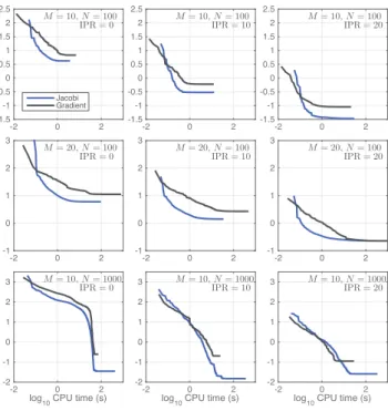
Fig. 2. FindingΦfor fixedVˆ. Objective function valueslog10(F(Φ))as

a function of CPU time for different valuesM, N(from top to bottom) and initializations forΦ(increasingly close to the ground-truthΦ∗_{, from left to}

right): Jacobi (blue) and Gradient (black) algorithm, respectively.

A large IPR value means Φ(0) and Φ∗ _{are close;}

Φ(0) is generated asΦ(0)=projOM(Φ∗+σB)where proj_OM denotes

the projection ontoOM _{[8], Bis a standard normal random}

matrix and σ_{>0is set to meet the desired IPR value.} The objective function values F(Φ) obtained for the two algorithms are plotted in Fig. 2 for several values of M, N

and IPR, as a function of CPU time. As expected, larger IPR values lead overall to solutions with smaller objective function value. A comparison of the two algorithms yields the following conclusions. First, with the proposed randomized Jacobi algorithm, a transform Φis obtained that corresponds with a local minimum of (9) that has a smaller objective function value than that returned by gradient descent. Sec-ond, the proposed algorithm is in general faster in finding a transform Φwith objective function below a given value, as indicated by the fact that in most of the cases plotted in Fig. 2, the blue curve (Jacobi) is consistently below the black curve (Gradient). Overall, these findings clearly demonstrate the practical benefits of the proposed randomized Jacobi algorithm for updatingΦ.

B. NMF with transform learning for audio data

We now study the full TL-NMF problem (2-3) with un-knowns (Φ,W_,H_{) for the decomposition of the toy piano}

sequence used in [5]. The audio sequence consists of four notes played all at once in the first measure and then by pairs in all possible combinations in the subsequent measures, see Fig. 3 (a) and (b). The audio signal was recorded live on a

(a) Score sheet

Fig. 3. Three representations of the piano data.

CPU time (s) 101 103 105 107 106 objective function IS-NMF TL-NMF Grad TL-NMF Jacobi CPU time (s) 101 103 105 107 106 fit CPU time (s) 101 103 105 107 106 L1 penalty

Fig. 4. Objective functionC(Φ,W,H₎, data fitting termD(|ΦY_|◦2 |WH₎

and sparsity termλ#H_#1with respect to CPU time.

real piano. The duration is 15.7 s with sampling frequency

fs = 16 kHz. The columns of matrix Y are composed of

adjacent frames of sizeM = 640(40ms) with50% overlap, windowed with a sine-bell. This leads to a total ofN = 785

frames.

We compare the performance and results of TL-NMF-Jacobi, TL-NMF-Gradient (the gradient descent method of [2]) and baseline (sparse) IS-NMF. The latter simply consists of running Algorithm 1 without step (U3) and with a fixed DCT transformΦ=ΦDCTdefined as

[ΦDCT]qm= (2M)− 1

2cos (π_{(q+ 1/2)(m+ 1/2)/M). (11)} The DCT spectrogram of the audio data is plotted in Fig. 3 (c). The three algorithms are run with K = 8. IS-NMF was run with τ _{= 10}−10_{, which ran in a few minutes on} a personal computer. TL-NMF-Gradient and TL-NMF-Jacobi were run for several days, reaching τ _{≈ 4·10}−7_{. Further,}

the parameters for TL-NMF-Jacobi are set to Nprop = 100,

R= 6and(a1, a2) = (0.3,0.7). All algorithms are initialized

with the same random factorsW_andH_{, and TL-NMF-Jacobi}

and TL-NMF-Gradient are initialized with the same random orthogonal matrixΦ. The hyper-parameter λ_{was set to 10}6_, like in [2]. 5 10 15 Component 1 IS-NMF 5 10 15 Component 2 5 10 15 Component 3 5 10 15 Component 4 5 10 15 Component 5 5 10 15 Component 6 5 10 15 Component 7 5 10 15 Component 8 time (s) 5 10 15 Component 1 TL-NMF Jacobi 5 10 15 Component 2 5 10 15 Component 3 5 10 15 Component 4 5 10 15 Component 5 5 10 15 Component 6 5 10 15 Component 7 5 10 15 Component 8 time (s)

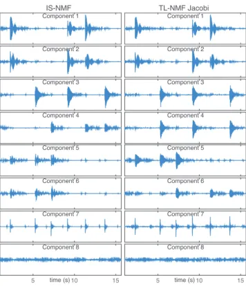
Fig. 5. Separated audio components using IS-NMF (left) and Jacobi TL-NMF (right), sorted by decreasing energy (from top to bottom). IS-NMF (resp., TL-NMF) splits the first (resp., second) and third notes over two components. In the two cases, component 7 extracts percussive sounds and component 8 contains residual noise.

Minimization of the objective function. Fig. 4 plots the

values of the objective functionC(Φ,W_,H_{), data fitting term}

D(|ΦX_|◦2_{)and sparsity term} λ₊H_{+1 as a function of CPU}

time and yields the following conclusions. Firstly, IS-NMF is of course considerably faster because Φ is fixed in its case. Then, Gradient is much slower than TL-NMF-Jacobi; it has not been able to reach a stationary point within the experiment’s runtime, and not even an objective function value below that of IS-NMF, despite the extra flexibility offered by learning Φ. In contrast, the proposed TL-NMF-Jacobi algorithm yields objective function values that are significantly below that reached by IS-NMF, already after a small fraction of the total runtime of the experiment. Finally, Fig. 4 shows that both the fit and the penalty term on H

are decreased along the iterations, which confirms the mutual influence of the sparsity of H _{and the learnt transform and}

dictionary.

Decomposition. Fig. 5 displays the 8 latent components

that can be reconstructed from the factorization returned by IS-NMF and by TL-NMF-Jacobi. The components have been reconstructed with standard Wiener filtering, inverse transformation and overlap-add [2], [5]. The set of com-ponents returned by the two methods are comparable and coherent: the piano notes, percussive sounds (hammer hitting the strings, sustain pedal release) and residual sounds are separated into distinct components. The corresponding audio

files are available online.1_{The audio quality of the components}

is satisfactory and comparable between the two methods, the components obtained with TL-NMF being a tiny bit fuzzy.

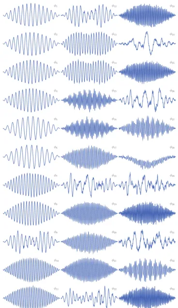
Learnt transform. We finally examine examples of the

atoms returned by TL-NMF (rows{φm}m ofΦ). Fig. 6

dis-plays the 33 atoms which most contribute to the audio signal (i.e., with largest values of+ΦY_{+2). As already observed in}

[2], the atoms adjust to the shape of the analysis window and come inquadrature pairs. As such, TL-NMF is able to learn a shift-invariant representation. Additionally, Fig. 6 shows that TL-NMF learns a variety of oscillatory patterns: regular tapered sine/cosine-like atoms (e.g.,φ₁-φ₈), harmonic atoms exhibiting slow (φ₉, φ₁₂-φ₁₄) to fast (φ₂₇, φ₃₂) amplitude modulations, atoms with little regularity (e.g.,φ₁₈,φ₂₂,φ₂₄) and atoms with uncommon structure (φ28). Atoms φ1 toφ8

fit to the fundamental frequencies of the 4 individual notes while the other atoms adjust to the specificities of the data (such as partials of the notes). The previous paragraph shows that they make sense of the data in their ability to produce a meaningful decomposition that accurately describes the data. We feel that it is quite remarkable to be able to learn such a structured transform from a random initialization.

IV. CONCLUSION

In this paper, we proposed a novel Jacobi algorithm for TL-NMF. Experiments with synthetic and audio data have illustrated its superior performance with respect to our pre-vious gradient-descent approach. In our setting it led to faster convergence and convergence to solutions with lesser objective values. We conjecture that the latter observation may be a consequence of the randomness element in the axes selection. The randomness is likely to improve the exploration of the non-convex landscape of the objective function. Despite TL-NMF-Jacobi being more efficient than TL-NMF-Gradient, it still runs very slow as it requires a few days to converge when applied to a few seconds audio signal (using a standard per-sonal computer). Future work will look into faster optimization using for example incremental/stochastic variants.

ACKNOWLEDGMENT

This work has received funding from the European Research Council (ERC) under the European Union’s Horizon 2020 research and innovation programme under grant agreement No 681839 (project FACTORY).

REFERENCES

[1] P. Smaragdis, C. F´evotte, G. Mysore, N. Mohammadiha, and M. Hoff-man, “Static and dynamic source separation using nonnegative factor-izations: A unified view,”IEEE Signal Processing Magazine, vol. 31, no. 3, pp. 66–75, May 2014.

[2] D. Fagot, H. Wendt, and C. F´evotte, “Nonnegative matrix factorization with transform learning,” inProc. IEEE International Conference on Acoustics, Speech and Signal Processing (ICASSP), 2018.

[3] S. Venkataramani and P. Smaragdis, “End-to-end source separation with adaptive front-ends,” arXiv:1705.02514, Tech. Rep., 2017.

[4] S. Ravishankar and Y. Bresler, “Learning sparsifying transforms,”IEEE Transactions on Signal Processing, vol. 61, no. 5, pp. 1072–1086, 2013.

1_{https://www.irit.fr/∼Cedric.Fevotte/extras/eusipco2018/audio.zip} φ1 φ2 φ3 φ4 φ5 φ6 φ7 φ8 φ9 φ10 φ11 φ12 φ13 φ14 φ15 φ16 φ17 φ18 φ19 φ20 φ21 φ22 φ23 φ24 φ25 φ26 φ27 φ28 φ29 φ30 φ31 φ32 φ33

Fig. 6. The 33 most energy-significant atoms learnt with TL-NMF-Jacobi.

[5] C. F´evotte, N. Bertin, and J.-L. Durrieu, “Nonnegative matrix factor-ization with the Itakura-Saito divergence. With application to music analysis,”Neural Computation, vol. 21, no. 3, pp. 793–830, Mar. 2009. [6] C. F´evotte and J. Idier, “Algorithms for nonnegative matrix factorization with theβ-divergence,”Neural Computation, vol. 23, no. 9, pp. 2421– 2456, 2011.

[7] A. Lef`evre, F. Bach, and C. F´evotte, “Itakura-Saito nonnegative matrix factorization with group sparsity,” inProc. IEEE International Confer-ence on Acoustics, Speech and Signal Processing (ICASSP), Prague, Czech Republic, May 2011.

[8] J. H. Manton, “Optimization algorithms exploiting unitary constraints,”

IEEE Transactions on Signal Processing, vol. 50, no. 3, pp. 635–650, 2002.

[9] G. H. Golub and C. F. Van Loan,Matrix computations, 3rd ed. The Johns Hopkins University Press, 1996.

[10] J.-F. Cardoso and A. Souloumiac, “Jacobi angles for simultaneous diagonalization,”SIAM Journal on Matrix Analysis and Applications, vol. 17, no. 1, pp. 161–164, 1996.