econ
stor
www.econstor.eu
Der Open-Access-Publikationsserver der ZBW – Leibniz-Informationszentrum Wirtschaft
The Open Access Publication Server of the ZBW – Leibniz Information Centre for Economics
Nutzungsbedingungen:
Die ZBW räumt Ihnen als Nutzerin/Nutzer das unentgeltliche, räumlich unbeschränkte und zeitlich auf die Dauer des Schutzrechts beschränkte einfache Recht ein, das ausgewählte Werk im Rahmen der unter
→ http://www.econstor.eu/dspace/Nutzungsbedingungen nachzulesenden vollständigen Nutzungsbedingungen zu vervielfältigen, mit denen die Nutzerin/der Nutzer sich durch die erste Nutzung einverstanden erklärt.
Terms of use:
The ZBW grants you, the user, the non-exclusive right to use the selected work free of charge, territorially unrestricted and within the time limit of the term of the property rights according to the terms specified at
→ http://www.econstor.eu/dspace/Nutzungsbedingungen By the first use of the selected work the user agrees and declares to comply with these terms of use.
zbw
Leibniz-Informationszentrum Wirtschaft Leibniz Information Centre for EconomicsChristmann, Andreas
Working Paper
Regression depth and support vector
machine
Technical Report / Universität Dortmund, SFB 475 Komplexitätsreduktion in Multivariaten Datenstrukturen, No. 2004,54
Provided in cooperation with:
Technische Universität Dortmund
Suggested citation: Christmann, Andreas (2004) : Regression depth and support vector machine, Technical Report / Universität Dortmund, SFB 475 Komplexitätsreduktion in Multivariaten Datenstrukturen, No. 2004,54, http://hdl.handle.net/10419/22567
Andreas Christmann
Abstract. The regression depth method (RDM) proposed by Rousseeuw and Hubert [RH99] plays an important role in the area of robust regression for a continuous response variable. Christmann and Rousseeuw [CR01] showed that RDM is also useful for the case of binary regression. Vapnik’s convex risk minimization principle [Vap98] has a dominating role in statistical ma-chine learning theory. Important special cases are the support vector mama-chine (SVM),ε−support vector regression and kernel logistic regression.
In this paper connections between these methods from different disciplines are investigated for the case of pattern recognition. Some results concerning the robustness of the SVM and other kernel based methods are given.
1. Introduction
Binary regression and statistical machine learning play a key role in theoretical
and applied statistics. In supervised learning we have a set of variables, sayX (the
predictors, the explanatory variables, or the inputs) which might have an influence
on one or on several response variables, say Y (the dependent variables or the
outputs). Then we are mainly interested in the conditional distribution ofY given
X. An example is the prediction of claim sizes and of the probability for a claim
in the context of motor vehicle insurance companies, cf. [Chr04]. In contrast
to that, in unsupervised learning the distinction between inputs and outputs can not be made in advance such that the joint distribution of all variables is of main interest. The number of variables can sometimes be extremely large in unsupervised statistical learning problems.
In this paper supervised statistical learning will be considered, where the single response variable is discrete. The minimum number of misclassifications achievable with affine hyperplanes on a given set of labeled points is of special importance.
The problem to determine this quantity exactly is NP-hard, see [HSvH95]. Hence,
there is a need to find reasonable and fast approximation procedures. One approach to approximate the minimum number of misclassifications achievable with affine
1991Mathematics Subject Classification. Primary 62G35, 62H30; Secondary 62G05, 47N30. Key words and phrases. Pattern recognition, kernel logistic regression, regression depth, ro-bustness, statistical machine learning, support vector machine.
This work was partially supported by the Deutsche Forschungsgemeinschaft (SFB 475, ”Re-duction of complexity in multivariate data structures”) and by the Forschungsband DoMuS from the University of Dortmund.
hyperplanes was proposed by Christmann and Rousseeuw [CR01]. The approach is
based on the regression depth method proposed by Rousseeuw and Hubert [RH99].
However, sometimes it is not sufficient to allow only affine hyperplanes for sep-arating two response groups. Therefore, we also treat the support vector machine
proposed by Vapnik [Vap98]. The SVM can be used with a linear kernel, but it
can also be used in combination with universal kernels as the Gaussian RBF ker-nel which allows more complex structures to separate both response groups. The SVM is one reference method well-known to be effective to fit complex and high dimensional data sets.
The rest of the paper is organized as follows. Section 2 gives the notions of
com-plete separation, quasicomcom-plete separation and overlap from [AA84] and [SD86].
Section 3 shows that the regression depth approach is useful for binary regression models to check whether the maximum likelihood estimate for the parameter vec-tor exists and how many data points are necessary to guarantee the existence. A connection between regression depth and overlap is shown and some algorithmic considerations are given. Section 4 briefly describes Vapnik’s convex risk mini-mization approach with special emphasis on the support vector machine. Section 5 describes the results of numerical comparisons between SVMs with a linear kernel and RDM. An example is given in Section 6 which shows that a SVM in combina-tion with the classical Gaussian RBF kernel can show an unstable behaviour with respect to training errors and test errors in certain multi-class classification prob-lems. Section 7 contains a brief summary of recent results concerning robustness properties of certain statistical machine learning methods based on kernels for the case of pattern recognition. Kernel logistic regression and the SVM are special cases. Section 8 gives some numerical results about prediction aspects of SVMs. Section 9 contains a discussion.
2. Separation and overlap
Generalized linear models are among the most popular approaches to model the occurrence of an event depending on a vector of explanatory variables, say
xi= (xi,1, . . . , xi,p−1)∈Rp−1. We will assume that there is also an intercept term.
Examples are the identification of risk factors for cancer in medical applications, estimating the probability of an insurance claim, the purchase of a product by a customer in direct marketing, or the probability that the price of a stock exceeds a previously defined value within one month taking into account general economic
data and indices measuring company performances. The responsesyiare commonly
assumed to be realizations of independent Bernoulli random variablesYi. Consider
a given set of observations Zn ={(xi,1, . . . , xi,p−1, yi);i = 1, . . . , n} ⊂Rp, where
yi ∈ {0,1} for i = 1, . . . , n. The goal is to find an affine hyperplane defined via
θ∈Rpsuch that a good classification of the responses is possible.
For the given data setZn, definencompleteas the minimum number of
misclas-sifications that any affine hyperplane must incur. In particular, if ncomplete = 0,
the data set iscompletely separated so that there exists a vectorθ∈Rp such that
(xi,1)θ0>0 if yi= 1
(2.1)
(xi,1)θ0<0 if yi= 0
for i= 1, . . . , n. A data set which is not completely separated is quasicompletely separated if there exists a vectorθ∈Rp\{0} such that
(xi,1)θ0≥0 if yi= 1
(2.3)
(xi,1)θ0≤0 if yi= 0
(2.4)
for alliand if there existsj∈ {1, ..., n} such that (xj,1)θ0= 0. A data set is said
to haveoverlapif there is no complete separation and no quasicomplete separation.
The quantityncomplete denotes the smallest number of observations whose removal
yields complete separation. The quantity noverlap denotes the smallest number of
observations whose removal yields complete or quasicomplete separation. For logis-tic regression with an intercept term, it is well-known that the classical maximum
likelihood estimate ofθdoes not exist if noverlap= 0, see [AA84] and [SD86].
The opposite holds true when training a single linear threshold function using
the Perceptron [Ros62] algorithm, which is guaranteed to converge only for data
sets with ncomplete = 0, cf. [Nov62]. The quantity ncomplete is a parameter in
bounds on the prediction error if one measures the quality of linear models
accord-ing to the empirical risk minimization principle, see [Vap98]. Unfortunately, the
problem of determining the exact minimum number of misclassifications ncomplete
based on an affine hyperplane for arbitrary dimensions is NP-hard.
Theorem 2.1. [HSvH95, Theorem 3.1]Let n disjoint points from Rp, each
labelled with response 0 or 1, and a bound k ≥ 1 be given. The problem to de-cide whether there is an affine hyperplane such that ncomplete ≤kis NP-complete.
The problem remains NP-complete if the points are only allowed to have integer coordinates.
The next section gives the definition of regression depth proposed by [RH99]
and shows a relationship to the notion of overlap in binary regression models.
3. Regression depth
Rousseeuw and Hubert [RH99] introduced the regression depth approach for
linear regression models. In the following we will consider the logistic regression model, although the method can be used for other binary regression models in
an analogous manner. Data sets analyzed with such models have the form Zn =
{(xi,1, . . . , xi,p−1, yi); i = 1, . . . , n} ⊂ Rp where yi ∈ {0,1} for i = 1, . . . , n. For
simplicity, we will assume that the design matrix has full column rank. Denote the
cumulative distribution function of the logistic distribution by Λ(z) = 1/[1 +e−z],
z∈R.
Definition 3.1. A vector θ = (θ1, . . . , θp) ∈ Rp is called a nonfit to Zn iff
there exists an affine hyperplaneV in x−space such that no xi belongs to V, and
such that the residual ri(θ) = yi− Λ((xi,1)θ0) > 0 for all xi in one of its open
halfspaces, andri(θ)<0 for allxi in the other open halfspace.
Definition3.2. Theregression depthof a fitθ= (θ1, . . . , θp)∈Rp relative
to a data setZn ⊂Rp is the smallest number of observations that need to be
re-moved to makeθa nonfit in the sense of Definition 3.1. Equivalently, rdepth(θ, Zn)
is the smallest number of residuals that need to change sign.
From Definition 3.2 it follows for logistic models that the regression depth of
set{(xi,1, . . . , xi,p−1,1−yi);i= 1, . . . , n}. Hence, the regression depth is invariant
with respect to different codings of the binary response variable.
There exists an interesting connection between regression depth and complete
separation. Define the horizontal hyperplane defined byθ∗ = (0, . . . ,0,0.5). Then
θ∗ is a nonfit iffn
complete= 0, and more generallyncomplete= rdepth(θ∗, Zn). This
implies thatncomplete can be computed with an algorithm for the regression depth
of a given hyperplane, cf. Christmann and Rousseeuw [CR01]. For p∈ {2,3,4}
the latter can be computed by theO(np−1log(n)) time algorithms of Rousseeuw
and Hubert [RH99] and Rousseeuw and Struyf [RS98]. For p≥3, [RS98]
con-structed a fast approximation algorithm based on appropriate projections for the
regression depth. The main idea of the algorithm for p ≥ 3 is to approximate
the p−dimensional regression depth by the minimum of certain two-dimensional
regression depths. We use
ncomplete = rdepth(θopt, Zn)
(3.1) = min θ∈Rprdepth(θ,Z˜n(θ)) (3.2) ≤ min θ∈B⊂Rprdepth(θ, ˜ Zn(θ)) =:ncomplete(B), (3.3) where (3.4) Z˜n(θ) ={((xi,1)θ0, yi);i= 1, . . . , n} ⊂R2, θ∈Rp,
andθoptis an optimal parameter vector.
The set B is determined via projections defined by a large number, say 104,
of random subsamples of the original data set. In a similar manner one can
also approximate noverlap by noverlap(B). Details of the algorithms are described
in Christmann and Rousseeuw [CR01]. Software to compute noverlap(B) and
ncomplete(B) written in R (packages noverlap and ncomplete from the website http://cran.r-project.org/) and in FORTRAN is available.
Of course, this approximation algorithm to computencomplete(B) is computer
intensive, if the dimensionsnor por the number of samples to be drawn, i.e. |B|,
are high. Further, drawing random subsamples of the original data set often result in affine hyperplanes for which the number of misclassifications is much higher than for the desired affine hyperplane.
Other determinations of the set B in (3.3) were investigated by [CFJ02]. A
naive alternative toncomplete(B) is to use only onespecial vectorbin (3.3). Define
b= ( ˆ θM L if ˆθM Lexists ˆ θ(k) otherwise,
where ˆθ(k) is the last vector computed by the usual Fisher-scoring algorithm to
compute the ML estimate in the logistic regression model after stopping due to
de-tection that there is no overlap in the data set. We computebby the SAS procedure
PROC LOGISTIC. This SAS procedure gives a warning if the data set has complete
separation or quasicomplete separation, but stores ˆθ(k)and the linear combinations
of (xi,1) and ˆθ(k). In the same manner, let s(b) be the asymptotic standard
er-ror of the ML estimate, if it exists, or the corresponding quantity evaluated for ˆ
θ(k). Of course, other programs to compute ML estimates in the logistic regression
model can also be used. The naive method ncomplete(b) often gives surprisingly
approximations ofncompletein an iterative manner as follows. The heuristic method
ncomplete(h) first tries to find a good approximation of ncomplete using the vector
b as a starting vector. Secondly, a grid search is done where sequentially some
of the components of b are set to zero. Then a local search again starting from
b is performed in the following way. We vary the parameter b componentwise in
discrete steps by a factor in the interval 0 to 3 taking into account the variability
measured by the quantities s(b). If an improvement occurs an additional
refine-ment is made starting from the best solution got so far. Finally the outcomes of all three methods (starting value, grid search, local search) are compared and the best solution is chosen. Of course, if during the whole procedure the best possible value ofncomplete= 0 is detected, the algorithms stops and outputs the current solution.
Rousseeuw and Christmann [RC03] proposed the hidden logistic regression
model. This model is strongly related to the logistic regression model. The advan-tage of the hidden logistic regression model is that robust estimation in that model is possible and that it circumvents the problem of non-existence of the estimates.
In the following section a relationship between the regression depth approach and the support vector machine is shown.
4. Convex risk minimization and SVM
In modern statistical machine learning theory the convex risk minimization
principle plays an important role. Vapnik [Vap98] proposed the support vector
machine, which is a special case and can be described as follows for the case of
pattern recognition. The responses are recoded as −1/+ 1 instead of 0/1. The
empirical regularized risk is defined by
(4.1) fˆn,λ= arg min f∈H 1 n n X i=1 L(yi, f(xi)) +λkfk2H,
where λ >0 is a penalizing constant, Y ={−1,+1}, L:Y ×R→R, is a convex
loss function, His a reproducing kernel Hilbert space with kernel k, andf ∈ H
is the function we like to estimate. The termλkfk2
H decreases the generalization
error and avoids over-fitting. The convexity ofLyields algorithmic advantages and
avoids computationally NP-hard problems. Popular loss functions depend onyand
f viav =yf(x) orv =y(f(x) +b), whereb ∈R is an additional intercept term.
The SVM uses the loss functionL(y, f(x) +b) = max(1−y[f(x) +b],0) such that
points are linearly penalized ifv :=y[f(x) +b]<1. Other methods based on the
convex risk minimization principle are kernel logistic regression, L2-SVM, modified
L2-SVM, modied Huber, and AdaBoost, see [Zha04].
The optimization problem (4.1) can be interpreted as a stochastic approxima-tion of the minimizaapproxima-tion of the theoretical regularized risk given in (4.2):
(4.2) fP,λ= arg min
f∈HEPL(Y, f(X)) +λkfk
2
H.
We denote by ( ˆfn,λ,ˆbn,λ) and (fP,λ, bP,λ) the corresponding quantities if we are
modellingf+binstead off, whereb∈Rdenotes in intercept term.
Decomposeθ in the slope part, say w= (θ1, . . . , θp−1), and the intercept part
θp. To describe the connections between the support vector machine and the
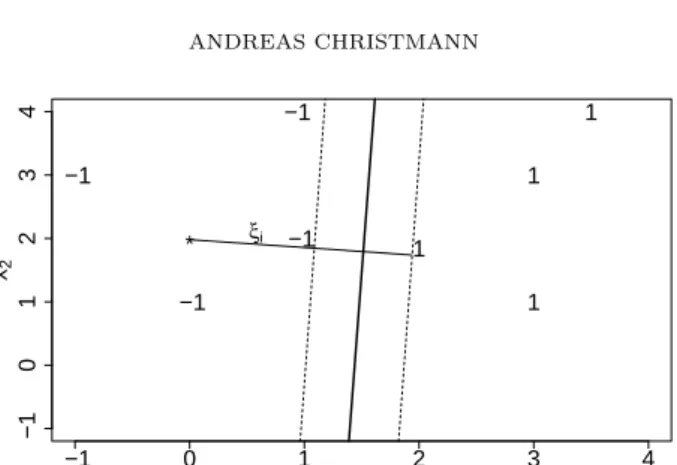
re-gression depth method, let us consider a two-dimensional data set, cf. Figure 1.
If the data point marked as∗ is equal to −1, then the solid line gives a complete
−1 0 1 2 3 4 −1 0 1 2 3 4 x1 x2 −1 * −1 −1 −1 1 1 1 1 ξi
Figure 1. Illustration of the support vector machine.
is called the margin. It is implicitly defined via the data points on its boundary. These data points are called support vectors. The margin is defined as the max-imum distance between parallel affine hyperplanes which separate both response groups.
However, if the data point marked as∗ is equal to +1, no complete separation
is possible by an affine hyperplane. The marked data point lies within the convex
hull of the opposite class with a distance proportional toξi minus the margin size.
The aim of the support vector machine is to maximize the width between all possible parallel affine hyperplanes which separate both response groups while
penalizing misclassifications by a large positive extra costC. DefineC= (2λn)−1.
Accordingly, the support vector machine solves the following quadratic optimization
problem (with intercept termb):
(P) minimize (w.r.t. w, b, ξ): 12||w||2+CP
iξi
subject to sign(yi)·(xi,1)θ0≥1−ξi and ξi≥0 .
Apart from some degenerate cases, the solution of the optimization is unique due
to the fact that the SVM uses a convex loss function. Here, C > 0 is a penalty
parameter specified by the data analyst to model an extra cost for errors. The
quantityξi must exceed unity for a misclassification to occur. Hence, the sum over
the slack parametersPi ξiis an upper bound on the number of training errors,cf.
[Bur98]. IncreasingC corresponds to a higher penalty to errors. In practice, one usually solves the following dual program
(D) minimize (w.r.t. α): 1
2α0Qα−α01
subject to α0y= 0 and0≤α≤C1 ,
where (Q)ij = yiyjx0ixj. Using the Karush-Kuhn-Tucker conditions of the dual
program (D), the quantitiesw,b, andξcan be computed in the following way. The
slope part ofθ is given by
(4.3) w=
n
X
i=1
αiyixi.
If 0< αi< C thenb=yi−xTiw. While this value ofbcorresponds to the solution
of the primal problem (P),bis commonly selected to directly minimize the number
of training errors for the givenw [Bur98]. This can easily be done after sorting
Of particular interest is the fact that the dual problem (D) depends only on in-ner products between vectors of explanatory variables. Substituting Mercer kernels for the simple dot product allows SVMs to efficiently estimate not only linear, but
also e.g. polynomial functions [BGV92]. Of special importance is the Gaussian
radial basis function (RBF) kernel
k(x, x0) = exp(−γkx−x0k2), γ >0,
which is a universal kernel on every compact subset ofRp in the sense of [Ste01].
If the number of observations nor the dimensionpis large, solving the
mini-mization problems (P) or (D) is computer-intensive. While some algorithms (e.g. PROC NLP or the IML function NLPQUA in SAS, Version 8) require storing the
huge matrix Q∈ Rn×n or the whole matrix specifying the constraints, SVMlight
[Joa99] is useful for solving the SVM optimization problem (D). SVMlight is
de-signed to efficiently handle problems with large p(e.g. 30,000) and large n (e.g.
100,000). To avoid computing and storing the full HessianQof (D), the algorithm
of SVMlightproceeds by decomposing the problem [OFG97]. Only a few variables
(q ≈10) are optimized at a time. Their selection is based on a steepest feasible
descent strategy. To reduce zig-zagging behavior, the original selection criterion [Joa99] can be modified. The working set is updated like a queue, with only two new variables entering in each iteration. Using this decomposition, the algorithm solves only small quadratic programs in each step. This leads to small memory
requirements. In particular, memory does not scale O(n∗n) like for algorithms
requiring the full Hessian, but typically only by O(n∗s), where s is the number
of support vectors. The number of support vectors is generally much lower than
n. The PR-LOQO optimizer developed by Smola [Smo98] can be used to increase
the numerical stability of SVMlight. In general, it is helpful to standardize all
explanatory variables in advance.
5. Comparison of SVM and RDM
A fair numerical comparison between the regression depth method and the support vector machine for the case of pattern recognition by affine hyperplanes is not easy. One reason is that the results can depend on the algorithms, on the actual implementations of the algorithms for numerical reasons, and of course on the considered data sets. Further, both approaches offer different options such as
the number of subsamples for RDM and the penalyzing constantC for SVM.
There are many software products for the support vector machine and related
methods. A good overview is given on the website www.kernel-machines.org.
Joachims [Joa99] showed that the computation time for the SVM depends heavily
on the algorithm and its implementation. His software SVMlight is fast even for
high dimensional data sets and was successfully applied for text mining. Sch¨olkopf
and Smola [SS02, p. 219] demonstrated that different SVM classifiers can yield
very different values for the test errors, ranging from 2.6% to 8.9% for the same
data set. Hastie, Tibshirani and Friedman [HTF01, p. 384f] compared the SVM
using polynomial kernels with degrees d ranging from 1 to 10 with BRUTO and
MARS for a simulated data set with 100 observations. It was shown that the test error of the SVM classifiers can depend not only on the kernel but also on the dimensionality of the problem.
Christmann, Fischer and Joachims [CFJ02] compared RDM, SVM, and linear discriminant analysis (LDA) for various benchmark data sets from robust logistic
regression. SVMlightwas used to compute the SVM. The main criterion was a low
misclassification error w.r.t. to affine hyperplanes. The computation time was the secondary criterion. Summarizing, RDM gave better results for small to moderate
sized data sets, say for data sets of dimensionp≤10 and up to 1,000 observations.
LDA showed the worst performance of the three methods. The misclassification
error based on LDA was even larger than the trivial upper bound for ncomplete
given by the minimum of the sum of the successes (yi = 1) and the sum of the
failures (yi= 0). Especially the heuristic algorithm ncomplete(h) gave good results.
It was somewhat surprising that the naive algorithm ncomplete(b) can outperform
the algorithm ncomplete(B) in certain situations. For more complex data sets, the
SVM usually performed well to approximate ncomplete and was fast. The results
for SVM depended on the penalyzing constantC. In generalC= 105/(p−1) gave
better approximations thanC= 103/(p−1), but the computation time increased.
However, SVM sometimes failed to detect that a data set had complete separation,
whereas ncomplete(b) was able to detect such situations. This was true also for
ncomplete(h), which is however more computer-intensive than ncomplete(b). There
do not yet exist algorithms to use RDM for very high dimensional data sets.
6. SVM and QDA
In this section we show that the SVM can be unstable with respect to training errors and test errors in certain multi-class classification problems. For simplicity, let us consider a two-dimensional problem with up to four classes without noise, although this phenomenon can also occur for more complex data sets. The
explana-tory variablesx1andx2are simulated independently from a uniform distribution on
the interval [−1,+1]. The four possible response classes are constructed as follows,
see Figure 2: yi= 0 (complement) if x2 1+x22<0.15 then yi = 1 (ball) if 0.15≤x2 1+x22<0.6 then yi = 2 (ring) if 0.25 +x1−x2<−0.5 then yi = 3 (triangle) .
We consider three situations: {ball, ring, complement}, {ball, triangle,
comple-ment}, and {ball, ring, triangle, complement}. For each situation 250 data sets
each with n = 1,000 observations were generated. Each data set was splitted by
random into a training data set with 700 observations and a test data set with 300
observations. An SVM with Gaussian RBF kernel and C = 104 and a quadratic
discriminant analysis (QDA) were done for each training data set. The R library
e1071 [LDH+03] was used to train the SVM. Then the corresponding training
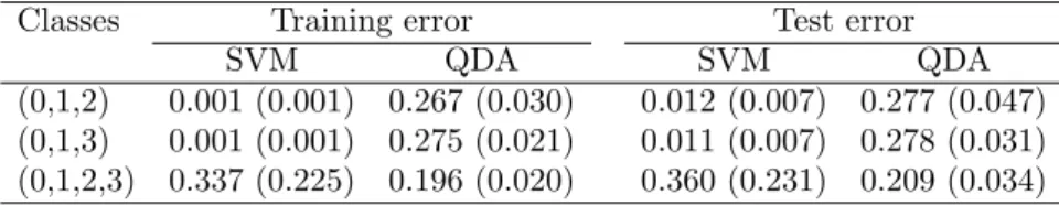
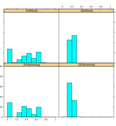
errors and test errors were computed, see Table 1. The SVM yields much better results than the QDA w.r.t. training errors and test errors for both classification problems with 3 response classes. Sometimes even the test errors based on SVM were zero, i.e. no misclassification happens, which did not happen for the QDA. However, for the classification problem with 4 response classes the SVM performed
oftenworsethan QDA and the predictions errors had a large variability, see Figure
3. The same figure shows that the SVM gave much smaller prediction errors than
the QDA for some of the 250 data sets. The predicted responses based on the
−1.0 −0.5 0.0 0.5 1.0 −1.0 −0.5 0.0 0.5 1.0 x1 x2 3 2 1 0
Figure 2. Illustration of simulated patterns.
Table 1. Averaged training and test errors for SVM and QDA.∗
Classes Training error Test error
SVM QDA SVM QDA
(0,1,2) 0.001 (0.001) 0.267 (0.030) 0.012 (0.007) 0.277 (0.047)
(0,1,3) 0.001 (0.001) 0.275 (0.021) 0.011 (0.007) 0.278 (0.031)
(0,1,2,3) 0.337 (0.225) 0.196 (0.020) 0.360 (0.231) 0.209 (0.034)
∗ Standard deviations are given in parenthesis.
the training data sets and the test data sets contained observations from all four response groups.
7. Robustness of the SVM
J.W. Tukey, one of the pioneers of robust statistics, already mentioned in 1960 [HRRS86, p. 21]:
A tacit hope in ignoring deviations from ideal models was that they would not matter; that statistical procedures which were optimal under the strict model would still be approximately optimal under the approximate model. Unfortunately, it turned out that this hope was often drastically wrong; even mild deviations often have much larger effects than were anticipated by most statisticians.
Different criteria have been proposed to define the notion of robustness in a
math-ematical way, e.g. Huber’s minimax approach [Hub64], Tukey’s sensitivity curve
[Tuk77], Hampels’s approach based on influence functions [Ham74, HRRS86],
the maxbias curve [Hub64, HRRS86], the finite sample breakdown point [DH83],
and the approach based on least favourable local alternatives [Rie94].
In contrast to robust statistics for parametric models such as linear regression or multivariate location and scatter problems the robustness of non-parametric and nonlinear methods as the SVM with Gaussian RBF kernels have not yet been
Error Count 0 50 100 150 200 250 0 0.2 0.4 0.6 0.8 1 SVM(training) QDA(training) SVM(test) 0 50 100 150 200 250 QDA(test) 0 0.2 0.4 0.6 0.8 1
Figure 3. Training errors (below) and test errors (above) for SVM (left) and QDA (right) for the case of four response classes.
studied in great detail. One of the difficulties is that the quantity of interest is no
longer a parameter vector, sayθ∈Rp, but a functionf ∈ Hor a pair (f, b)∈ H×R,
whereHdenotes the reproducing kernel Hilbert space.
For the case of pattern recognition Christmann and Steinwart [CS04] showed
that some of the general robustness approaches can be successfully applied to a broad class of methods based on Vapnik’s convex risk minimization principle. The following theorem gives the influence function of such methods. The Dirac
distri-bution in the pointzis denoted by ∆z.
Theorem 7.1. [CS04] Let L:Y ×R→[0,∞) be a convex and twice contin-uously differentiable loss function, whereY ={−1,+1}. Furthermore, letX ⊂Rn
be a closed or open subset, H be a RKHS of a bounded continuous kernel on X, andP be a distribution onX×Y. We defineG:R× H → Hby
G(ε, f) := 2λf+ E(1−ε)P+ε∆zL 0(Y, f(X))Φ(X) which implies ∂G ∂ε(0, fP,λ) =−EP[L 0(Y, f P,λ(X))Φ(X)] +L0(zy, fP,λ(zx))Φ(zx).
DefineS:H → Hby
S:= ∂G
∂H(0, fP,λ) = 2λidH+ EPL 00(Y, f
P,λ(X))hΦ(X), .iΦ(X).
Then the influence function of the classifiers based on (4.2) exists for all z = (zx, zy)∈X×Y and is given by
(7.1) IF(z;T,P) =−S−1◦ ∂G
∂ε(0, fP,λ).
Remark 7.2. The influence function derived in Theorem 7.1 depends on the point z = (zx, zy) only by the term L0(zy, fP,λ(zx))Φ(zx). Note the similarity of
this term to the weighting scheme used by influence function of Mallows type
M-estimators. In our case the weighting of zx is of course performed in the feature
space. This term can be bounded by choosing a loss function with a bounded
derivativeL0 and a bounded and continuous kernelk. An example is kernel logistic
regression with the Gaussian RBF kernel.
Summarizing the results given in [CS04] for pattern recognition, it turned
out that the influence functions offP,λ and (fP,λ, bP,λ) exist, and if bounded and
continuous kernels are used in combination with appropriate loss functions, the influence function, the maxbias, and the sensitivity curve can be uniformly bounded.
Note that Theorem 7.1 is a result concerning the robustness of fP,λ but not
for the prediction of Y, i.e. sign(fP,λ(x)). In the next section some preliminary
numerical results are given for such predictions.
8. Prediction aspects of SVM
The goal of this section is to study the effect which a single data point can have
on the prediction areas for the responsey computed by the SVM.
We generated a data set withn= 500 data pointsxifrom a bivariate Student’s
t3 distribution with location parameter µ = (0,0) and scatter matrix Σ. The
diagonal elements of Σ were set to 1, whereas the off-diagonal elements were set
to 0.25. The responses yi were generated from a logistic regression model with
intercept for the parameter vectorθ= (−1,1) andb= 1, such that P(Yi= +1) =
[1 + exp(−[b+x0
iθ])]−1 andP(Yi=−1) = 1−P(Yi= +1).
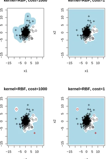
The upper part of Figure 4 shows that the choice of the penalizing constantC
can be quite important for making predictions based on a support vector machine with a Gaussian RBF kernel. This holds true especially if predictions are made for
a response with anx−value outside the bulk of the x−values of the training data
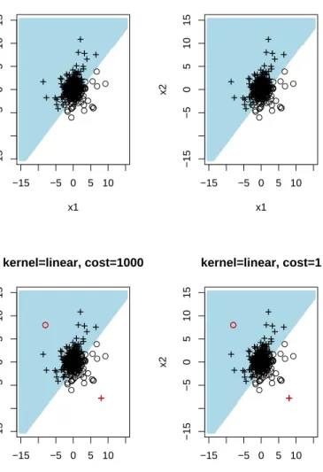
set. Such observations are often called leverage points. In this sense, the SVM can produce unstable predictions and should be used with some care. In the lower part of Figure 4, corresponding prediction areas are given if two of the data points are moderate outliers. The SVM with a universal Gaussian RBF kernel accommodates outliers due to the consistency property. The corresponding SVM based prediction areas for a linear kernel are quite different, see Figure 5.
Similar sensitivity analyses were done for some other situations: increased sam-ple size, situations where a comsam-plete separation of both response groups is possible, and for a multivariate normal distribution instead of a multivariate Student
distri-bution to generate thex−values. The results are not given here because the results
−15 −5 0 5 10 −15 −5 0 5 10 15 kernel=RBF, cost=1000 x1 x2 ++++++++++++++ + + + + +++ + + + + + + + + + ++ + +++ + + + + + ++++++ +++ + + + + + ++++ + +++ + + + + + + + + + ++ ++++++++++ ++ ++ + + + + + + + + + + + ++ ++++++ +++++++++++ + + + ++ ++ + +++ + + + ++ + +++ + ++ +++ + + + + +++++++++++ +++ + ++ + + +++ + + + +++ + +++ + + + + + ++++ ++ + + ++ + + + + + + + + +++ ++++ + ++++ ++ ++ ++++++++ + + + ++ + ++ ++++ ++++++++ + + + + ++++ + ++++++ ++++++++++ + + ++ + + +++ ++ + + + + + + + ++++++ + +++ + + ++++++++++++ + ++++++ + +++ ++ + +++ + + ++ + + + + −15 −5 0 5 10 −15 −5 0 5 10 15 kernel=RBF, cost=1 x1 x2 ++++++++++++++ + + + + +++ + + + + + + + + + ++ + +++ + + + + + +++ +++ +++ + + + + + + +++ + +++ + + + + + + + + +++ +++++ + + +++ ++ +++ + + + + + + + + + + ++ ++++++ +++++++++++ + + + ++ ++ + +++ + + + ++ + ++ + + ++ +++ + + + + +++++++++++ +++ + ++ + + +++ + + + +++ + +++ + + + + + ++++ ++ + + ++ + + + + + + + + +++ +++ + + ++++ ++ ++ ++++++++ + + + ++ + ++ ++++ ++++++++ + + + + ++++ + ++++++ ++++++++++ + + ++ + + +++++ + + + + + + + ++++++ + +++ + + ++++++++++++ + ++++++ + +++ ++ + +++ + + ++ + + + + −15 −5 0 5 10 −15 −5 0 5 10 15 kernel=RBF, cost=1000 x1 x2 + ++ ++++ ++++ ++++ + + + + ++++ + + + + + + + + ++ + + ++++++ ++ +++++ + ++++ + + + + + + ++++ + +++ + + + +++++++++++ + + + + + + + + +++ ++ ++ + + + + ++ +++ + + ++ + + +++ ++++++ ++++++++++++ + + +++ ++ + ++ + + + +++++++ + ++ ++++ + + + + +++++++++++ +++ + + ++ + ++ +++ + ++ + + + + + + + + +++ + + + ++ ++++ + ++ + ++ ++ + + + + + + +++ + + ++ +++++ + ++++ ++ ++ +++++++++++ + + ++ ++++ + + ++ +++++ +++++ + + + + ++ + + +++ ++ ++ +++++++ +++++++ +++ + ++ + ++++ ++++ ++ +++ + + ++ +++ + + ++++ + + +++++++++++++ + + + +++++++++ + + ++ ++ + +++ + + + ++ + + + + + + −15 −5 0 5 10 −15 −5 0 5 10 15 kernel=RBF, cost=1 x1 x2 + ++ ++ ++ + +++ ++++ + + + + ++++ + + + + + + + + ++ + + ++++++++ +++++ + ++++ + + + + + + ++++ + +++ + + + + ++++++++++ + + + + + + + + +++ ++ +++ + + + ++ +++ + + ++ + + +++ ++++++ ++++++++++++ + + +++ ++ + ++ + + + +++++++ + ++ ++++ + + + + +++++++++++ +++ + + ++ + ++ +++ + ++ + + + + + + + + +++ + + + ++ ++++ + ++ + ++ ++ + + + + + + +++ + + ++ +++ ++ + ++++ ++ ++ +++++++++++ + + ++ ++++ + + ++ +++++ +++++ + + ++++ + + +++++ ++ +++++++ +++++++ + ++ + ++ + ++++++ +++++++ + + ++ +++ + + ++++ + + +++++++++++++ + + + +++++++++ + + ++ ++ + +++ + + + ++ + + + + + +
Figure 4. SVM based prediction areas using a Gaussian RBF kernel. Upper: simulated data set. Lower: simulated data set
with two moderate outliers located at xA = (8,−8) with yA = 1
and xB = (−8,8) with yB = −1. Legend: + for y = 1, ◦ for
y=−1. The prediction area for ˆy= 1 is shaded.
9. Discussion
In this paper pattern recognition problems were considered because they play an important role in many areas for applied statistics.
Firstly, the case was treated that the response groups should be separated by
affine hyperplanes. Relationships between the regression depth method [RH99],
−15 −5 0 5 10 −15 −5 0 5 10 15 kernel=linear, cost=1000 x1 x2 ++++++++++++++ + + + + +++ + + + + + + + + + ++ + +++ + + + + + ++++++ +++ + + + + + ++++ + +++ + + + + + + + + + ++ ++++++++++ ++ ++ + + + + + + + + + + + ++ ++++++ +++++++++++ + + + ++ ++ + +++ + + + ++ + +++ + ++ +++ + + + + +++++++++++ +++ + ++ + + +++ + + + +++ + +++ + + + + + ++++ ++ + + ++ + + + + + + + + +++ ++++ + ++++ ++ ++ ++++++++ + + + ++ + ++ ++++ ++++++++ + + + + ++++ + ++++++ ++++++++++ + + ++ + + +++ ++ + + + + + + + ++++++ + +++ + + ++++++++++++ + ++++++ + +++ ++ + +++ + + ++ + + + + −15 −5 0 5 10 −15 −5 0 5 10 15 kernel=linear, cost=1 x1 x2 ++++++++++++++ + + + + +++ + + + + + + + + + ++ + +++ + + + + + +++ +++ +++ + + + + + + +++ + +++ + + + + + + + + +++ +++++ + + +++ ++ +++ + + + + + + + + + + ++ ++++++ +++++++++++ + + + ++ ++ + +++ + + + ++ + ++ + + ++ +++ + + + + +++++++++++ +++ + ++ + + +++ + + + +++ + +++ + + + + + ++++ ++ + + ++ + + + + + + + + +++ +++ + + ++++ ++ ++ ++++++++ + + + ++ + ++ ++++ ++++++++ + + + + ++++ + ++++++ ++++++++++ + + ++ + + +++++ + + + + + + + ++++++ + +++ + + ++++++++++++ + ++++++ + +++ ++ + +++ + + ++ + + + + −15 −5 0 5 10 −15 −5 0 5 10 15 kernel=linear, cost=1000 x1 x2 + ++ ++++ ++++ ++++ + + + + ++++ + + + + + + + + ++ + + ++++++ ++ +++++ + ++++ + + + + + + ++++ + +++ + + + +++++++++++ + + + + + + + + +++ ++ ++ + + + + ++ +++ + + ++ + + +++ ++++++ ++++++++++++ + + +++ ++ + ++ + + + +++++++ + ++ ++++ + + + + +++++++++++ +++ + + ++ + ++ +++ + ++ + + + + + + + + +++ + + + ++ ++++ + ++ + ++ ++ + + + + + + +++ + + ++ +++++ + ++++ ++ ++ +++++++++++ + + ++ ++++ + + ++ +++++ +++++ + + + + ++ + + +++ ++ ++ +++++++ +++++++ +++ + ++ + ++++ ++++ ++ +++ + + ++ +++ + + ++++ + + +++++++++++++ + + + +++++++++ + + ++ ++ + +++ + + + ++ + + + + + + −15 −5 0 5 10 −15 −5 0 5 10 15 kernel=linear, cost=1 x1 x2 + ++ ++ ++ + +++ ++++ + + + + ++++ + + + + + + + + ++ + + ++++++++ +++++ + ++++ + + + + + + ++++ + +++ + + + + ++++++++++ + + + + + + + + +++ ++ +++ + + + ++ +++ + + ++ + + +++ ++++++ ++++++++++++ + + +++ ++ + ++ + + + +++++++ + ++ ++++ + + + + +++++++++++ +++ + + ++ + ++ +++ + ++ + + + + + + + + +++ + + + ++ ++++ + ++ + ++ ++ + + + + + + +++ + + ++ +++ ++ + ++++ ++ ++ +++++++++++ + + ++ ++++ + + ++ +++++ +++++ + + ++++ + + +++++ ++ +++++++ +++++++ + ++ + ++ + ++++++ +++++++ + + ++ +++ + + ++++ + + +++++++++++++ + + + +++++++++ + + ++ ++ + +++ + + + ++ + + + + + +
Figure 5. SVM based prediction areas using a linear kernel. Up-per: simulated data set. Lower: simulated data set with two
moderate outliers located at xA = (8,−8) with yA = 1 and
xB = (−8,8) withyB =−1. Legend: + for y= 1, ◦ for y=−1.
The prediction area for ˆy= 1 is shaded.
and quasicomplete separation [AA84, SD86] in the context of logistic regression
were investigated.
We also considered the case that the response groups should be separated by
more complex functionsf. Therefore, we treated the support vector machine with
the more flexible Gaussian RBF kernel. Robustness issues for the estimation off
were considered. Some numerical examples were also given for the case of predic-tion.
References
[AA84] A. Albert and J.A. Anderson, On the existence of maximum likelihood estimates in logistic regression models, Biometrica71(1984), 1–10.
[BGV92] B. E. Boser, I. M. Guyon, and V. N. Vapnik,A training algorithm for optimal margin classifiers, Proceedings of the 5th Annual ACM Workshop on Computational Learning Theory (Pittsburgh, PA) (D. Haussler, ed.), ACM Press, July 1992, pp. 144–152. [Bur98] C. J. C. Burges,A tutorial on support vector machines for pattern recognition, Data
Mining and Knowledge Discovery2(1998), 121–167.
[CFJ02] A. Christmann, P. Fischer, and T. Joachims,Comparison between various regression depth methods and the support vector machine to approximate the minimum number of misclassifications, Computational Statistics17(2002), 273–287.
[Chr04] A. Christmann,An approach to model complex high-dimensional insurance data, All-gemeines Statistisches Archiv4(2004).
[CR01] A. Christmann and P.J. Rousseeuw,Measuring overlap in logistic regression, Compu-tational Statistics and Data Analysis37(2001), 65–75.
[CS04] A. Christmann and I. Steinwart, On robust properties of convex risk minimization methods for pattern recognition, Journal of Machine Learning Research5(2004), 1007– 1034.
[DH83] D.L. Donoho and P.J. Huber, The notion of breakdown point, A Festschrift for Erich L. Lehmann (Belmont, California, Wadsworth) (P.J. Bickel, K.A. Doksum, and J.L. Hodges Jr., eds.), 1983, pp. 157–184.
[Ham74] F.R. Hampel, The influence curve and its role in robust estimation, Journal of the American Statistical Association69(1974), 383–393.
[HRRS86] F.R. Hampel, E.M. Ronchetti, P.J. Rousseeuw, and W.A. Stahel,Robust statistics. the approach based on influence functions, Wiley, New York, 1986.
[HSvH95] K.U. H¨offgen, H.-U. Simon, and K.S. van Horn,Robust trainability of single neurons, Journal Computer and System Sciences50(1995), 114–125.
[HTF01] T. Hastie, R. Tibshirani, and J. Friedman, The elements of statistical learning, Springer, New York, 2001.
[Hub64] P.J. Huber,Robust estimation of a location parameter, Annals of Mathematical Sta-tistics35(1964), 73–101.
[Joa99] T. Joachims,Making large-scale svm learning practical, Advances in Kernel Methods - Support Vector Learning (MIT Press, Cambridge, Massachusetts) (B. Sch¨olkopf, C. Burges, and A. Smola, eds.), 1999, pp. 41–56.
[LDH+03] F. Leisch, E. Dimitriadou, K. Hornik, D. Meyer, and A. Weingessel,R package e1071,
2003, http://cran.r-project.org.
[Nov62] A. Novikoff,On convergence proofs on perceptrons, Proceedings of the Symposium on the Mathematical Theory of AutomataXII(1962), 615–622.
[OFG97] E. Osuna, R. Freund, and F. Girosi,An improved training algorithm for support vector machines, Neural Networks for Signal Processing VII — Proceedings of the 1997 IEEE Workshop (New York) (J. Principe, L. Gile, N. Morgan, and E. Wilson, eds.), IEEE, 1997, pp. 276–285.
[RC03] P.J. Rousseeuw and A. Christmann, Robustness against separation and outliers in logistic regression, Computational Statistics & Data Analysis43(2003), 315–332. [RH99] P.J. Rousseeuw and M. Hubert,Regression depth, Journal of the American Statistical
Association94(1999), 388–433.
[Rie94] H. Rieder,Robust asymptotic statistics, Springer, New York, 1994. [Ros62] F. Rosenblatt,Principles of neurodynamics, Spartan, New York, 1962.
[RS98] P.J. Rousseeuw and A. Struyf,Computing location depth and regression depth in higher dimensions, Statistics and Computing8(1998), 193–203.
[SD86] T.J. Santner and D.E. Duffy,A note on a. albert and j.a. anderson’s conditions for the existence of maximum likelihood estimates in logistic regression models, Biometrika73 (1986), 755–758.
[Smo98] A. J. Smola,Learning with kernels, Ph.D. thesis, Technische Universit¨at Berlin, 1998. [SS02] B. Sch¨olkopf and A.J. Smola, Learning with kernels. support vector machines,
[Ste01] I. Steinwart,On the influence of the kernel on the consistency of support vector ma-chines, Journal of Machine Learning Research2(2001), 67–93.
[Tuk77] J.W. Tukey,Exploratory data analysis, Addison-Wesley, Reading, Massachusetts, 1977. [Vap98] V.N. Vapnik,Statistical learning theory, Wiley, 1998.
[Zha04] T. Zhang, Statistical behaviour and consistency of classification methods based on convex risk minimization, Annals of Statistics32(2004), 56–134.
Department of Statistics, University of Dortmund, 44221 Dortmund, GERMANY
Current address: Department of Statistics, University of Dortmund, 44221 Dortmund, GER-MANY