Chinese
Journal of
Aeronautics
Chinese Journal of Aeronautics 22(2009) 160-166 www.elsevier.com/locate/cjaApplication of Least Squares Support Vector Machine for
Regression to Reliability Analysis
Guo Zhiwei, Bai Guangchen*
School of Jet Propulsion, Beijing University of Aeronautics and Astronautics, Beijing 100191, China
Received 23 May 2008; accepted 17 September 2008
Abstract
In order to deal with the issue of huge computational cost very well in direct numerical simulation, the traditional response surface method (RSM) as a classical regression algorithm is used to approximate a functional relationship between the state vari-able and basic varivari-ables in reliability design. The algorithm has treated successfully some problems of implicit performance function in reliability analysis. However, its theoretical basis of empirical risk minimization narrows its range of applications for the regression model. In contrast to classical algorithms, the support vector machine for regression (SVR) based on structural risk minimization has the excellent abilities of small sample learning and generalization, and superiority over the traditional regres-sion method. Nevertheless, SVR is time consuming and huge space demanding for the reliability analysis of large samples. This article introduces the least squares support vector machine for regression (LSSVR) into reliability analysis to overcome these shortcomings. Numerical results show that the reliability method based on the LSSVR has excellent accuracy and smaller com-putational cost than the reliability method based on support vector machine (SVM). Thus, it is valuable for the engineering ap-plication.
Keywords:mechanism design of spacecraft; support vector machine for regression; least squares support vector machine for regression; Monte Carlo method; reliability; implicit performance function
1. Introduction1
Reliability is an issue of high significance in engi-neering design, when the variables are conspicuously random[1]. Generally, it is a crucial aspect to get the
performance function in reliability analysis. It is very convenient to manage the reliability analysis based on performance function, whereas, the performance func-tion is formulated with an explicit funcfunc-tion. However, the performance function is always expressed in im-plicit function in practical problems. Theoretically, any reliability analysis method based on explicit perform-ance function is also suitable for implicit performperform-ance function[1-2]. Yet, due to the unknown performance
function, there are still many unconquerable problems in practical treatment, which restrict such as first order reliability method (FORM), second order reliability method (SORM), etc. In order to conquer these prob-lems brought about by implicit function, since 1990s
*Corresponding author. Tel.: +86-10-82317418.
E-mail address: [email protected]
Foundation item:National High-tech Research and Development Pro-gram (2006AA04Z405)
doi: 10.1016/S1000-9361(08)60082-5
various kinds of regression methods have been con-stantly used to solve the reliability analysis problem induced by implicit performance function[3]. The clas-sic method is response surface method (RSM)[4-7].
Al-though a lot of excellent researches have been done to improve the accuracy and adaptability of reliability analysis on the RSM, many problems are still remain-ing in the practical applications[8]. For example,
re-sponse surface function can only approximate per-formance function well around the design points. J. E. Hurtado[3] has explained that the drawback of RSM is
owing to its being a rigidly non-adaptive regression technique in the statistical learning perspective. At present, a new kind of regression model—support vector machine (SVM) has been applied to reliability analysis to solve those drawbacks of the traditional regression models.
SVM is a kind of statistical learning method. It comprises support vector machine for classification (SVC) and support vector machine for regression (SVR). C. M. Rocco and J. A. Moreno[9] firstly
intro-duced SVM method into the reliability analysis. J. E. Hurtado and D. A. Alvarez[10] treated reliability analy-sis as a pattern recognition and adopted SVM in con-junction with stochastic finite element to analyze struc-
tural reliability. Combing with SVR, H. S. Li and Z. Z. Lu[8] first presented SVR-based FORM (SVR-FORM)
and SVR-based Monte Carlo simulation (SVR-MCS) methods.
In the theoretical perspective, SVM is a learning al-gorithm based on statistical learning theory being suit-able for small sample. It transforms the problem of searching for the optimal hyperplane between two classes into the problem of solving the maximal classi-fication margin. The maximal margin problem is actu-ally a quadratic programming (QP) problem subjected to the inequality constraint[11]. In spite of SVM’s many
advantages, one problem is that the size of the matrix of QP problem is directly proportional to the number of training points, so that the standard QP program package cannot be used even for moderately large data sets[12]. It means that regarding the reliability analysis
of large samples, the existing SVM methods are time consuming and huge space demanding. To offset these disadvantages, this article introduces the least square support vector machine for regression (LSSVR) into the reliability analysis and puts forward LSSVR-based MCS (LSSVR-MCS) reliability analysis method, and contrasts the time consumption of standard SVR-MCS with that of LSSVR-MCS.
2. SVR
From a certain kind of assumed distribution: P(x, y), n
R
x , yR, the sampling points {( , )}xi yi i 1,2, ,l are generated. If there is a set of functions that map a point in the space Rn onto the space R[13-16]:
{ ( , ), | : n }
F f x w w/ f R oR (1) where / is a set of parameters, w an undetermined parameter vector.
Then, the regression subject is to find a function
f F which makes Eq.(2) shown as below have the lowest expected risk
( ) ( ( , ))d ( , )
R f
³
l yf x w P x y (2) where l y( f( , ))x w is an error function and defined in SVR as( ( , )) max{0, ( , ) }
l y f x w y f x w H (3) where H > 0. Function f can be determined by the following method.
If sampling points are assumed in a linear relation, then the regression function can be written as
( , ) +
f x w w x b (4) But in most cases, the input sampling points and out-put sampling points are assumed in a nonlinear relation. For this case, SVR method maps each sampling point by a nonlinear function Monto the higher dimensional space and conducts linear regression in the higher
di-mensional space, so as to attain the original space nonlinear regression effect. Now the function f is re-written as
( , ) ( ) +
f x w w M x b (5) Thus, the problem of solving the regression function can be transformed to obtain the following optimized solution
2
1 min
2 w (6) The corresponding constraints are
( ) +i b y i dH (i 1, 2, , )l
wM x (7)
Considering the possible errors and introducing two slack variables
*
, 0 ( 1, 2, , )
i i i l
[ [ t the optimization function is then as follows
2 * 1 1 min ( ) 2 l i i i J [ [ w
¦
(8) The corresponding constraints are* * ( ) ( ) , 0 ( 1, 2, , ) i i i i i i i i b y y b i l [ H [ H [ [ ½ d ° d ° ¾ t ° ° ¿ w x w x M M (9)
For obtaining the solution of this QP, the Lagrange function is introduced 2 * * 1 1 * 1 * 1 1 ( , , , ) ( ) 2 ( ( ) ) ( ( ) ) ( ) l i i i l i i i i i l i i i i i l i i i i L b y b y b J [ [ D [ H D [ H K [ [
¦
¦
¦
¦
w w w x w x D D M M (10) where , * 0 ( 1, 2, , ) i i i l D D t .In the optimization process, the inner product cal-culation in the higher dimensional space is always in-volved. Using a kernel function ( ,\ x xi j) to replace the inner product ( )M xi M( )xj , the Lagrange duality problem is expressed as * * * , , 1 * * 1 1 1 min[ ( )( ) ( , ) 2 ( ) ( )] l i i j j i j i j l l i i i i i i i y D D D D \ H D D D D
¦
¦
¦
x x D D (11) subjected to the constraints½ ° ° ° ° °° ¾ ° ° ° ° ° °¿ * * 1 ( ) 0 (0 , ; 1, 2, , ) l i i i i i i l D D dD D dJ
¦
(12)After getting the optimized solution D , D*, and b,
the regression estimating function is as follows
* SV ( ) ( ) ( , ) i i i i f D D \ b
¦
x x x x (13) where SV is a set of support vector for a given sample set.3. LSSVR
The algorithm of the LSSVR is to solve the follow-ing optimization question[11,17]
T 2 , 1 1 min ( , ) 2 l i i J J
¦
e w e w e w w (14) whereas, satisfying the equality constraintsT ( ) ( 1, 2, , )
i i i
y w M x b e i l (15) The polynomial of Lagrange duality problem is
T 1 ( , , , ) ( , ) l i( ( )i i i) i L w b eD J w e
¦
D w M x b e y (16) Its optimization conditions are1 1 T ( ) 0 0 0 0 ( ) 0 ( 1, 2, , ) l i i i l i i i i i i i i i L L b L e e L b e y i l D D D J D w o w w o w w o w w o w
¦
¦
0 w x w w x M M (17)Eq.(17) can also be written as the following linear equations set T T b J ª ºª º ª º « » « » « » « » « » « » « » « » « » « » « » « » « » ¬ ¼ ¬ ¼ ¬ ¼ 0 0 0 0 0 0 0 1 0 0 0 1 0 I Z w e I I y Z I D (18) where T 1 2 [e e el] e T 1 2 [y y yl] y T [1 1 1] 1 T 1 2 [D D Dl] D T 1 2 [ ( ) ( ) ( )]l Z M x M x M x
By eliminating e and w, and utilizing the following
Mercer condition,
T
( ( )) ( ) ( , ) ( , 1, 2, , )
kj k j k j k j l
: M x M x \ x x (19)
the resultant equations set is then only related to D and
b. Therefore, Eq.(18) is transformed into
T 1 b J ª º ª º ª º « » « » « » ¬ ¼ ¬ ¼ « » ¬ ¼ 0 1 0 1 : I D y (20)
On the assumption that A :J1I and because
A is a symmetric and positive semi-definite matrix, A–1
does exist. Thus, the solution of Eq.(20) can be for-mulated as T 1 T 1 1( ) b b ½ ° ¾ ° ¿ 1 1 1 1 A y A A y D (21) Using the first equation of Eq.(17) to replace the w in Eq.(5) and using Eq.(19), the desired regression function can be written as
1
( ) l i ( , )i i
f x
¦
D \ x x b (22) where Di and b are the solutions of Eq.(21).4. Numerical Examples
In this section, the reliability method is adopted which is based on LSSVR-MCS method. In the reli-ability analysis, it is mainly using LSSVR to create a surrogate model of physical performance function. From the method provided by Ref.[8], the sampling points are selected randomly according to the distribu-tion of the random variables and then introduced into the ready-made LSSVR surrogate model to get the response values. The failure probability can be calcu-lated by f f ( ( ) 0) ( ( ) 0) N P P g P f N d | d | x x (23)
where g(x) is physical performance function, f (x) sur-rogate function created by LSSVR, N the total sam-pling number according to the random variable prob-ability density and 10 000 random samples are taken, and Nf the number of sampling points within the zone
of f (x) 0.
Example 1 Quadratic limit state reliability analy-sis
Eq.(24) is a quadratic limit state function (LSF) and is often taken to examine the accuracy of the implicit limit state reliability analysis method[7-8].
2 1 2 4 ( ) 4 ( 1) 25 g x x x (24) where x1 and x2 obey the standard normal distribution.
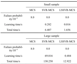
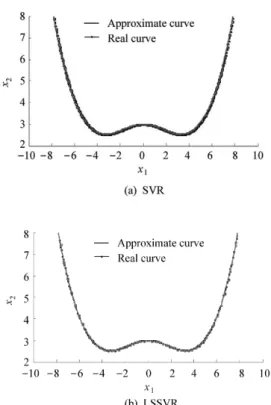
the real curves of LSF are shown in Fig.1. The ap-proximate curves are obtained on the basis of SVR and LSSVR respectively and only twenty samples are cho-sen as training points. Two hundred of the samples are taken into account as a large sample case and the cor-responding figures are shown in Fig.2. The results of failure probability and computation cost for different number of samples and methods are summarized in Table 1.
Fig.1 Comparison of real and approximate curves of LSF for small sample (Example 1).
Fig.2 Comparison of real and approximate curves of LSF for large sample (Example 1).
Table 1 Comparison of results (Example 1)
Small sample MCS SVR-MCS LSSVR-MCS Failure probabil-ity/10–4 8.0 8.0 8.0 Learning time/s 0.282 0.016 Total time/s 6.407 1.656 Large sample MCS SVR-MCS LSSVR-MCS Failure probabil-ity/10–4 8.0 8.0 8.0 Learning time/s 69.016 0.484 Total time/s 130.250 12.922
Example 2 Quartic limit state reliability analysis For general purpose, Eq.(25) shows a quartic LSF
2 4 1 1 2 ( ) 2 exp( ) ( ) 10 5 x x g x x (25) where x1 and x2 are standard normal distribution
vari-ables. The comparison of real and approximate curves of LSF for both SVR and LSSVR are demonstrated in Fig.3 corresponding to the case of a small samples. The corresponding figures for a large sample are shown in Fig.4.
In case of Example 2, the results of failure probabil-ity and computation cost are listed in Table 2 for dif-ferent sample sizes and difdif-ferent methods, respectively.
Fig.3 Comparison of real and approximate curves of LSF for small sample (Example 2).
Fig.4 Comparison of real and approximate curves of LSF for large sample (Example 2).
Table 2 Comparison of results (Example 2)
Small sample MCS SVR-MCS LSSVR-MCS Failure probabil-ity/10–3 1.84 1.80 1.80 Learning time/s 0.297 0.016 Total time/s 6.484 1.703 Large sample MCS SVR-MCS LSSVR-MCS Failure probabil-ity/10–3 1.84 1.80 1.80 Learning time/s 75.531 0.469 Total time/s 136.047 12.907
Example 3 Reliability analysis of three-span con-tinuous beam
The result of reliability analysis for three-span beam is presented in Ref.[18]. Its LSF is
4 ( , , ) 0.006 9 360 L qL g q E I EI (26) where q denotes the distributed loads, E the modulus of elasticity, and I the moment of inertia. These vari-ables are distributed normally and independent of each other, and their distribution parameters are given in Table 3. In order to highlight the distinction of com-putation cost between SVR-MCS and LSSVR-MCS, five hundred of the samples are chosen as training samples. Table 4 lists the comparison of results derived from LSSVR-MCS and SVR-MCS.
Table 3 Distribution parameters of variables (Example 3)
Random variable Mean Standard deviation
q/(kN·m–1) 10 0.4
E/(107kN·m–2) 2 0.5
I/(10–4 m4) 8 1.5
Table 4 Comparison of results for large sample (Example 3) MCS SVR-MCS LSSVR-MCS Failure probabil-ity/10–4 8.96 9.00 9.00 Learning time/s 1 140.352 4.125 Total time/s 1 287.875 29.188
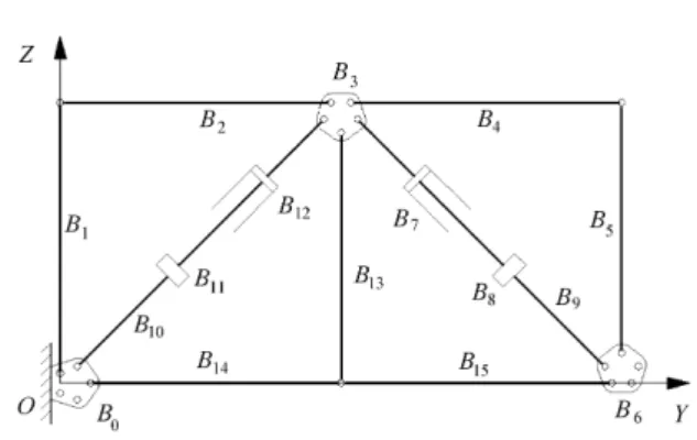
Example 4 Reliability analysis of deployable me- chanism for huge space station
The deployable mechanism for huge space station is an important object in the research and development of space vehicles. It is a planar flexible multibody system. Figs.5-6 are the initial state and deployable state of this mechanism, respectively.
The flexible deployable mechanism is static in ini-tial state. It takes 30 s to start the iniini-tial state and transmit to the end. From 0 s to 10 s, the mechanism is driven by a momentum Md and then the mechanism
completes the rest of the process by inertia. The resis-tant momentum Mf and assembling error (showed by
the coordinates xp and yp) are taken into account during
the dynamic simulation. L. C. Yu[19] pointed out that
the maximum horizontal velocity of component B5 is
less than 60 mm/s in order to avoid coupling vibration in the deploying process. The flexible model of the mechanism is established using virtual prototyping software ADAMS. The variables listed in Table 5 are assumed to be normal distribution and the maximum horizontal velocity of component B5 is chosen as the
design objective during the numerical simulation. It takes around 2 min to accomplish the simulation of one group of samples by a computer with CPU 2GHz/
Fig.6 Deployable state of a deployable mechanism[19].
2G and 3 h are required to accomplish the simulation of 100 samples. Therefore, it is a time consuming method to apply MCS method directly to the me-chanical reliability analysis when large samples are needed. One hundred groups of samples derived from ADMAS simulation are taken as the training samples of SVR and LSSVR to create the surrogate models of the deployable mechanism. The results based on dif-ferent methods are listed in Table 6.
Table 5 Distribution parameters of variables (Example 4)
Random variable Mean Deviation
Md –4.0 N·mm 0.1 (N·mm)2
Mf 0.5 N·mm 0.025 (N·mm)2
t 10 s 0.25 s2
xp –246.858 mm 4 mm2
yp 643.209 mm 4 mm2
Table 6 Comparison of results (Example 4)
SVR-MCS LSSVR-MCS Failure probability 0.045 5 0.046 5
Learning time/s 8.997 8 0.149 1
Total time/s 39.656 5.575
The results obtained from LSSVR-MCS and SVR- MCS are nearly the same as that given by L. C. Yu in Ref.[19], in which the failure probabilities based on MCS and artificial netural network-based Monte Carlo simulation (ANN-MCS) are 0.046 3 and 0.045 0, re-spectively.
5. Conclusions
This article puts forward a revised reliability analy-sis based on SVM, namely LSSVR-MCS method. The LSSVR-MCS method transforms the inequality con-straint of SVR-MCS into equality concon-straint so as to change the solving algorithm of the support vector machine from quadratic programming to a linear equa-tion set and make the solving approach easier. The numerical results indicate:
(1) With the increase of number of training samples, the approximate LSF curve approaches the real one
more closely.
(2) Whatever the computation cost, failure probabil-ity or approximate curve, the results obtained from LSSVR-MCS are as good as that obtained from SVR- MCS for small sample.
(3) In the case of large sample, LSSVR-MCS method is obviously superior to SVR-MCS method in computation cost.
References
[1] Gomes H M, Awrcuh A M. Comparison of response surface and neural network with other methods for structural reliability analysis. Structural Safety 2004; 26(1): 49-67.
[2] Schueremans L, Gemert D V. Benefit of splines and neural networks in simulation based structural reliabil-ity analysis. Structural Safety 2005; 27(3): 246-261. [3] Hurtado J E. An examination of methods for
approxi-mating implicit limit state function from the viewpoint of statistical learning theory. Structural Safety 2004; 26(3): 271-293.
[4] Bucher C G, Bourgund U. A fast and efficient response surface approach for structural reliability problems. Structural Safety 1990; 7(1): 57-66.
[5] Rajashekhar M R, Ellingwood B R. A new look at the response surface approach for reliability analysis. Structural Safety 1993; 12(3): 205-220.
[6] Kim S, Na S. Response surface method using vector projected sampling points. Structural Safety 1997; 19 (1): 3-19.
[7] Guan X L, Melchers R E. Effect of response surface parameter variation on structural reliability estimates. Structural Safety 2001; 23(4): 429-444.
[8] Li H S, Lu Z Z. Support vector regression for structural reliability analysis. Acta Aeronautica et Astronautica Sinica 2007; 28(1): 94-99. [in Chinese]
[9] Rocco C M, Moreno J A. Fast monte carlo reliability evaluation using support vector machine. Reliability Engineering & System Safety 2002; 76(3): 237-243. [10] Hurtado J E, Alvarez D A. Classification approach for
reliability analysis with stochastic finite-element mod-eling. Journal of Structural Engineering 2003; 129(8): 1141-1149.
[11] Jiang J Q, Wu C G, Song C Y, et al. Adaptive and itera-tive gene selection based on least squares support vec-tor regression. Journal of Information & Computational Science 2006; 3(3): 443-451.
[12] Chua K S. Efficient computations for large least square support vector machine classifiers. Pattern Recognition Letters 2003; 24(1-3): 75-80.
[13] Vapnik V N. The nature of statistical learning theory. New York: Springer-Verlag, 1995.
[14] Vapnik V N. Statistical learning theory. New York: John Wiley, 1998.
[15] Cortes C, Vapnik V N. Support vector networks. Ma-chine Learning 1995; 20(3): 273-297.
[16] Vapnik V N. An overview of statistical learning theory. IEEE Transaction on Neural Networks 1999; 10(5): 988-999.
[17] Suykens J A K, Lukas L, Vandewalle J. Sparse ap-proximation using least squares support vector machine. The 2000 IEEE International Symposium on Circuits and Systems. 2000; 2: 757-760.
[18] Li H S, Lu Z Z, Yue Z F. Support vector machine for structural reliability analysis. Applied Mathematics and Mechanics 2006; 27(10): 1295-1303.
[19] Yu L C. Dynamic reliability analysis, design and simu-lation of flexible mechanism. PhD thesis, Beijing Uni-versity of Aeronautics and Astronautics, 2006. [in Chi-nese]
Biographies:
Guo Zhiwei Born in 1981, he received B.S. and M.S. from Beijing University of Aeronautics and Astronautics in 2003 and 2005 respectively, and now he is a Ph.D. candidate. He has already published six technical papers on mechanical or aeronautical journals. He was granted Airbus scholarship for his researching effort. His main research interest focuses on
structural and mechanical reliability.
E-mail: [email protected]
Bai Guangchen Born in 1962, he received Ph.D. in 1993, and now is a professor of Beijing University of Aeronautics and Astronautics. He has published seventy technical papers in mechanical or aeronautical journals. His main research interests are reliability engineering and optimization design. His research activities were supported by National Natural Science Foundation of China, National Postdoctoral Science Foundation of China, Aeronautical Supporting Technology Foundation of China and National High-tech Research and Development Program of China.
E-mail: [email protected]
CALL FOR PAPERS
The 3rd International Basic Research Conference on
Rotorcraft Technology
A third conference will be held in celebration of the 24th anniversary of the first conference at the same univer-sity, Nanjing University of Aeronautics and Astronautics in 1985.
Nanjing, China, Nov. 9 - 11, 2009
Sponsored by
The American Helicopter Society, the Pennsylvania State University Nanjing University of Aeronautics and Astronautics and the
Chinese Society of Aeronautics and Astronautics
Subject matter/scope/conference theme:
A comprehensive array of advanced rotorcraft basic research technologies will be emphasized, including RUAV (Rotary Unmanned Air Vehicles) and MAV (Micro Air Vehicles). Interdisciplinary technologies in the areas of rotorcraft aerody-namics, dynamics & vibration, acoustics, flight controls, HUMS, structures, propulsion and drive systems, ice protection, and avionics will be covered. The reported work will include analytical capabilities, new experimental studies, new vehicle design concepts, and correlation/validation efforts. Analytical papers may range from basic aerodynamics, including low Reynolds numbers, to results of comprehensive analysis programs. Experimental papers will span model- to full-scale wind tunnel and flight test programs. Revolutionary new rotorcraft concepts or applications of emerging technologies to new rotorcraft missions will be addressed.
Abstract Submittal:
Abstracts should be written in English and should be no longer than five papers, including background, approach, key re-sults, conclusions, and sample supporting figures.
The approach and results should be presented in sufficient detail to allow the reviewer to determine the quality, scope, sig-nificance and current status of the work that will be described in the final paper. Priority will be given to papers in which significant results and conclusions are provided. Submit abstracts, including paper title, author(s), name(s), address, phone, fax and e-mail address no later than May 30, 2009. Electronic submittal is strongly preferred.
Completed Papers:
Authors will be notified of final selection by June 30, 2009. Presentations will be given in an open forum and all papers will be published in the conference proceedings. Final papers are due August 31, 2009, preferably in electronic format. The author is responsible for any necessary clearances and approvals.
All questions should be directed to the Technical Chairman: Prof. GAO Zheng, NUAA, [email protected], 86-25- 84892120, and Prof. Ken Brentner, Penn State University, AHS Journal Editor-in-Chief, (814)865-7092, [email protected], or to the Arrangements Chairman: Prof. XIA Pinqi, NUAA, [email protected], 86-25-84892491.
Abstracts should be submitted to Prof. Edward Smith, Penn State, [email protected], or to Prof. XIA Pinqi, NUAA, [email protected]