Wavelet-support vector machine for forecasting palm oil price

Wavelet-support vector machine for forecasting palm oil price

Ani Shabri

_{, Mohd Fahmi Abdul Hamid}

a _{Department of Mathematical Science, Faculty of Science, Universiti Teknologi Malaysia, 81310 UTM Johor Bahru, Johor, Malaysia} b _{UNITAR Foundation School, UNITAR International University, 47301 Petaling Jaya, Selangor, Malaysia}

* Corresponding author: [email protected]; [email protected]

Article history Received 3 May 2019 Revised 18 July 2019 Accepted 12 September 2019 Published Online 25 June 2019

Abstract

This study examines the feasibility of applying Wavelet-Support Vector Machine (W-SVM) model in forecasting palm oil price. The conjunction method wavelet-support vector machine (W-SVM) is obtained by the integration of discrete wavelet transform (DWT) method and support vector machine (SVM). In W-SVM model, wavelet transform is used to decompose data series into two parts; approximation series and details series. This decomposed series were then used as the input to the SVM model to forecast the palm oil price. This study also utilizes the application of partial correlation-based input variable selection as the preprocessing steps in determining the best input to the model. The performance of the W-SVM model was then compared with the classical SVM model and also artificial neural network (ANN) model. The empirical result shows that the addition of wavelet technique in W-SVM model enhances the forecasting performance of classical SVM and performs better than ANN.

Keywords: Support vector machine, discrete wavelet transform, artificial neural network, partial correlation variable selection, palm oil price

© 2018 Penerbit UTM Press. All rights reserved

INTRODUCTION

Forecasting agriculture commodities price can be very challenging due to its behavior that subject to significant price fluctuations. Like any other agriculture commodities, the determination of palm oil price is based on the complex relationship between multiple factors such as demand and supply rate, price of substitute product such as soybean price, crude oil price, time-lag etc. The non-stationary characteristics in the time series data implies that its distribution is changing over time. Due to the characteristics of its data, forecasting palm oil price poses noteworthy challenge for researcher to come out with the most accurate forecast.

There are several models that commonly used by researcher to forecast palm oil price. One of it is univariate model, Autoregressive Integrated Moving Average (ARIMA) (Ahmad et al., 2014; Arshad & Ghaffar, 1986; Khin et al., 2013; Nochai & Nochai, 2006). This Box-Jenkins methodology is widely used because of its simplicity and the underlying idea behind this model is forecast value is based on the past value and its error. The other most common model used is econometric regression model (multivariate model) (Abdullah & Lazim, 2006; Khin et al., 2013; Shamsudin & Arshad, 1999; Shamsudin et al., 1988). In econometric model, researchers try to explain the variation of palm oil price forecast based on several other determinant variables, which cannot be done by univariate model. Both ARIMA and econometric model are considered as traditional model which undeniably can produce a reliable result. By contrast to this traditional method, there were also researcher that use more advance technique to forecast palm oil price that is by machine learning method. Karia et al. (2013), Khamis & Wahab (2016) and Nor et al. (2014) in their study utilize artificial neural network methodology in forecasting palm oil price and they found out the result was plausible.

In forecasting, there is another advance machine learning tool that widely being used which is Support Vector Machine (SVM). It was developed by Vapnik and his colleagues in 1998 (Drucker et al., 1997) and its originally been used in classification problem. Unlike the neural network models that implement the empirical risk minimization principle, SVM implements the structural risk minimization principle which seeks to minimize an upper bound of the generalization error rather than minimize the training error. Therefore, SVM model will produce more general solutions which are global optimum while neural network models may tend to fall into a local optimal solution and tendencies of overfitting are less-likely to occur in SVM (Kim, 2003). There are number of studies that have shown SVM as a vigorous tool in time series forecasting such as in (Chen et al., 2004; Kim, 2003; Min & Lee, 2005; Tay & Cao, 2001). Therefore, this study will try to implement SVM methodologies as a forecasting model to palm oil price.

In recent years, the application of wavelet transform has gained a lot of attention in time series forecasting (Deo et al., 2016; Hamid & Shabri, 2017; Hsieh et al., 2011; Jammazi et al., 2015; Kim, 2003; Kisi & Cimen, 2011; F. Liu & Fan, 2006; Liu et al., 2011; Shabri & Samsudin, 2014; Tang et al., 2009). The attention given to wavelet transform in time series forecasting is because the effectiveness of this method in dealing with non-stationary data. For example, Shabri and Samsudin (2014) proposed a hybrid model integrating of wavelet transform and ANN to forecast crude oil price. In their study, wavelet transform used as the data prepossessing technique to capture the multi-scale features of a time series, which is used to decompose the data price series. The new series from wavelet decomposition then used as the input for ANN model, and the result shows that the proposed hybrid model performs better than conventional ANN. Khandelwal et al., (2015) used discrete wavelet transform to decompose data series into

linear and nonlinear component which respectively pick up the higher and lower frequency components. Then those frequencies are reconstructed through the inverse of wavelet transform and used as the input for ARIMA and ANN. The empirical result from this study (Khandelwal et al., 2015) shows that their proposed method has yielded notably better forecasts than ARIMA, ANN and hybrid’s model of ARIMA and ANN. The error measurement (MSE) for their proposed method reduced by 56% compared to ARIMA and ANN, and 44% compared to the hybrid model of ARIMA and ANN.

The objective of this paper is to examine the feasibility of applying the combination of discrete wavelet transform (DWT) and support vector machine (SVM) in palm oil forecasting by comparing it with a neural network model as a benchmark. Due to the nature of palm oil price characteristics that depends on multi-variable factors including the lagged variable of its predictor, this model will have a large number of predictors that some of it might not be significant. Therefore, this paper also will utilize input variable selection based on partial correlation of palm oil price and its predictors.

This paper consists of five sections. Section 2 will discuss about the theoretical background of SVM, ANN, DWT and input variable selection (IVS). Section 3 describes the research design and the research process of this study. Section 4 will describe the result and discussion of the findings. Section 5 will present the conclusion of this study.

THEORETICAL BACKGROUND Support vector machine regression

SVM is a supervised learning algorithm that widely used in classification and regression problem. The basic idea of SVM is to map input vector from training data into higher dimensional feature space via a specific function and then construct a separating hyperplane with maximum margin in the feature space. This maximum margin hyperplane gives maximum separation between decision class and the training samples that are the closest to the hyperplane are called support vectors. In support vector regression machine, the idea is to determine a function that can approximate future value accurately.

Given set of data points {𝑥𝑖, 𝑦𝑖}𝑖=1𝑙 where each 𝑥𝑖∈ 𝑅𝑛 denotes the

input space that has corresponding target value 𝑦𝑖∈ 𝑅 and 𝑙 is the size

of training data. The general function of support vector regression (SVR) take form:

𝑓(𝑥) = (𝑤 ∙ 𝜙(𝑥)) + 𝑏 (1)

where 𝑤 ∈ 𝑅𝑛_{, 𝑏 ∈ 𝑅, and 𝜙 denotes the non-linear transformation}

from 𝑅𝑛 to higher dimensional feature space. Coefficient of 𝑤 and 𝑏 can be determined by minimizing the regression risk

𝑅𝑟𝑒𝑔(𝑓) = 𝐶 ∑ Γ(𝑓(𝑥𝑖− 𝑦𝑖)) 𝑙

𝑖=0

+1

2∥ 𝑤 ∥2 (2) where Γ(∙) is the cost function, 𝐶 is a constant, and vector 𝑤 can be written in term of data points:

𝑤 = ∑(𝛼𝑖− 𝛼𝑖∗) 𝑙

𝑖=1

𝜙(𝑥𝑖) (3)

Substitute (3) into (1), the general equation can be written as:

𝑓(𝑥) = ∑(𝛼𝑖− 𝛼𝑖∗) 𝑙

𝑖=1

(𝜙(𝑥𝑖) ∙ 𝜙(𝑥)) + 𝑏

= ∑𝑙𝑖=1(𝛼𝑖− 𝛼𝑖∗)𝑘(𝑥𝑖, 𝑥) + 𝑏 (4)

The dot product in (4) is replaced by a kernel function 𝑘(𝑥𝑖, 𝑥),

which enable the dot product to be transformed into higher dimensional space. There are three type of kernels that commonly used in SVM that

is linear, Radial Basis Function (RBF) and polynomial (Wu, Ho, & Lee, 2004). This study will utilize all these kernel, and the kernel functions are shown in

Table 1.

Table 1 Kernel function.

Kernel Function

Linear 𝑥 ∗ 𝑦

Radial Basis Function exp{−𝛾 | 𝑥 − 𝑥𝑖 |2}

Polynomial [(𝑥 ∗ 𝑥𝑖) = 1]𝑑

The cost function that is used in minimizing the regression risk are measured using Vapnik’s 𝜀-insensitive loss function. The cost function takes the following form:

Γ(𝑓(𝑥) − 𝑦) = {𝑓(𝑥) − 𝑦 − 𝜀, 𝑓𝑜𝑟 𝑓(𝑥) − 𝑦 ≥ 𝜀

0, 𝑜𝑡ℎ𝑒𝑟𝑤𝑖𝑠𝑒 (5)

Solving the optimization problem, Equation (2) and (5) can be minimized 1 2∑ (𝛼𝑖∗− 𝛼𝑖)(𝛼𝑗∗− 𝛼𝑗) 𝑙 𝑖,𝑗=1 𝑘(𝑥𝑖, 𝑥𝑗) − ∑ 𝛼𝑖∗(𝑦𝑖− 𝜀) − 𝛼𝑖( 𝑙 𝑖=1 𝑦𝑖+ 𝜀) (6) subject to ∑𝑙𝑖=1𝛼𝑖− 𝛼𝑖∗= 0, 𝛼𝑖, 𝛼𝑖∗∈ [0, 𝐶] (7)

where 𝛼𝑖 and 𝛼𝑖∗ is the Lagrange multipliers that represent the solution

to the above quadratic equation which also act as forces that push prediction towards actual value 𝑦𝑖. Only non-zero values of the Lagrange multipliers are useful to determine the regression function and known as support vectors, that is requirement 𝑓(𝑥) − 𝑦 ≥ 𝜀 being fulfilled. Constant 𝐶 in Equation (2) determines the penalties to estimation error. Large value of 𝐶 assigns higher penalties to error which reflect to lower generalization of regression function while small value of 𝐶 allows minimization of margin with error, thus reflect to higher generalization.

Artificial neural network (ANN)

The fundamental principle of ANN is based on biological nervous system that acts as a non-linear mapping with a loose structure. It has been widely used in numbers of field such as pattern recognition, data processing, robotics etc. ANN also shows a huge success in the field of forecasting especially in non-linear modelling (Abedinia et al., 2016; Assis et al., 2010; Noori et al., 2010). The fundamentals concept in ANN is basically involving feeding the model with some input vectors, the model then will calculate the error in the output layer then some adjustment is made to the weight of the network to minimize the error.

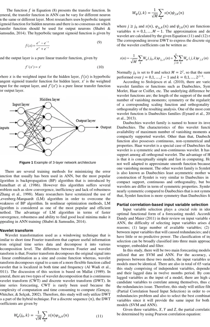
No priori assumption about the properties of data is needed and unlike the traditional statistical models, ANN is a non-parametric data-driven model which makes it less susceptible to the problem of model misspecification. The most common ANN model architecture consists three layers; input layer where the data introduced to the model, hidden layer where the data is processed, and output layer where the result is produced. The example of a three layers feed forward network architecture as shown in Figure 1.

Based on the model in (8), 𝑌 denoted as the output and 𝑥𝑖 is the

input to the system. 𝑤𝑖 and 𝛽 represents the connection weight and the

bias (threshold) respectively.

𝑌 = 𝑓[∑(𝑥𝑖𝑤𝑖) + 𝛽] 𝑙

𝑖=1

The function 𝑓 in Equation (8) presents the transfer function. In general, the transfer function in ANN can be vary for different neuron in the same or different layer. Most researchers uses hyperbolic tangent sigmoid function for hidden neurons and there is no consensus on which transfer function should be used for output neurons (Shabri & Samsudin, 2014). The hyperbolic tangent sigmoid function is given by

x x x x e e e e x f _     ) ( (9)

and the output layer is a pure linear transfer function, given by ' ) ' ( ' x x f  (10)

where 𝑥 is the weighted input for the hidden layer, 𝑓(𝑥) is hyperbolic tangent sigmoid transfer function for hidden layer, 𝑥’ is the weighted input for the output layer, and 𝑓′(𝑥’) is a pure linear transfer function for output layer.

Figure 1 Example of 3-layer network architecture There are several training methods for minimizing the error function that usually has been used in ANN, but the most popular algorithm is backpropagation (BP) algorithm that is introduced by Rumelhart et al. (1986). However this algorithm suffers several problem such as slow convergence, inefficiency and lack of robustness (Zhang et al., 1998). Many researchers have scrutinized the use of Levenberg-Marquardt (LM) algorithm in order to overcome the weakness of BP algorithm. In nonlinear optimization methods, LM algorithm is considered as one of the most popular and efficient method. The advantage of LM algorithm in terms of faster convergence, robustness and ability to find good local minima make it appealing in ANN training (Shabri & Samsudin, 2014).

Wavelet transform

Wavelet transformation used as a windowing technique that is similar to short time Fourier transform that capture useful information from original time series data and decompose it into various decomposition level. The difference between Fourier and wavelet transform is that; Fourier transform decomposes the original signal into a linear combination as a sine and cosine function whereas, wavelet transform decomposes signal to a sum of a more flexible function called wavelet that is localized in both time and frequency (Al Wadi et al., 2011). The discussion of this section is based on Mallat (1989). In general, there are two types of wavelet decomposition that is continuous wavelet transform (CWT) and discrete wavelet transform (DWT). In time series forecasting, CWT is rarely been used because the complexity of computation and time consuming to compute (Gençay, Whitcher, & Selçuk, 2002). Therefore, this study will only utilize DWT as a part of the hybrid technique. For a discrete sequence (𝑛), the DWT coefficients are given by

𝑊𝜑(𝑗0, 𝑘) = 1 √𝑀∑ 𝑠(𝑛)𝜑𝑗0,𝑘(𝑛) 𝑛 (11) 𝑊𝜓(𝑗, 𝑘) = 1 √𝑀∑ 𝑠(𝑛)𝜓_𝑛 𝑗,𝑘(𝑛) (12) where 𝑗 ≥ 𝑗0 and 𝑠(𝑛), 𝜑𝑗0,𝑘(𝑛) and 𝜓𝑗,𝑘(𝑛) are functions of discrete

variables 𝑛 = 0,1, … , 𝑀 − 1. The approximation and details of the wavelet are calculated by the given Equation (11) and (12) respectively. The corresponding inverse DWT to express the discrete signal in terms of the wavelet coefficients can be written as:





Normally 𝑗0 is set to 0 and select 𝑀 = 2𝐽, so that the summations are

performed over 𝑗 = 0,1, … , 𝐽 − 1 and 𝑘 = 0,1, … , 2𝑗−1_.

According to Stolojescu et al. (2010), there are various types of wavelet families or functions such as Daubechies, Symlet, Meyer, Morlet, Haar or Coiflet, etc. The underlying difference between these wavelet functions are; the length of the support of the mother wavelet; number of vanishing moments; symmetry or the regularity; existence of a corresponding scaling function and orthogonality or the bi-orthogonality of the resulting analysis. One of the most commonly used wavelet function is Daubechies families (Eynard et al., 2011; Ramesh et al., 2013).

Daubechies wavelet family is named to honor its inventor, Ingrid Daubechies. The characteristics of this wavelet function are the availability of maximum number of vanishing moments and they are compactly supported wavelet. Other than that, Daubechies wavelet function also possesses continuous, non-symmetrical and orthogonal properties. Haar wavelet is a special case of Daubechies families. Haar wavelet is a symmetric and non-continuous wavelet. It has the shortest support among all orthogonal wavelet. The advantage of Haar wavelet is that it is conceptually simple and fast in computing. However, it is not well adapted to approximate smooth function because it only has one vanishing moment. The other wavelet family is Symlet function. It is also known as Daubechies least asymmetric mother wavelet. The construction of Symlet is very similar to Daubechies in term of the compact support, continuous and orthogonality, but both of these wavelets are differ in term of symmetric properties. Symlet function is nearly symmetric compared to Daubechies that is not symmetric, means that, Symlet function is more symmetry than Daubechies function.

Partial correlation-based input variable selection

Input variable selection plays a crucial role in identifying the optimal functional form of a forecasting model. According to May, Dandy and Maier (2011) in their review on input variable selection for ANN, the difficulty of selecting input variables arises due to three reasons; (1) large number of available variables; (2) correlation between input variables that will caused redundancies; and (3) variables have little or no predictive power. The classification of input variable selection can be broadly classified into three main approaches that are wrapper, embedded and filter.

In this study, there will be two main forecasting models that will be utilized that are SVM and ANN. For the accuracy, comparative purposes between these two models, the input variables used for both models must be identical. There are also in total of 65 variables used in this study comprising of independent variables, dependent variables and their lagged data in twelve months period. By considering the lagged variables as the input of a model, there are high chances that candidate variables to correlate among themselves, thus contribute to the redundancies issue. Therefore, this study will utilize filter approach (Partial Correlation based Input Selection) in order to overcome the redundancies problem and also to select the best combination of input variables since it will provide the same input for both forecasting models (SVM and ANN).

Given three variables, 𝑋, 𝑌 and 𝑍, the partial correlation 𝜌𝑋𝑌∙𝑍 can

𝜌𝑋𝑌∙𝑍=

𝜌𝑋𝑌− 𝜌𝑋𝑍𝜌𝑌𝑍

√(1 − 𝜌𝑋𝑍2 )(1 − 𝜌𝑌𝑍2 )

(14) Partial correlation 𝜌𝑋𝑌∙𝑍 measures the correlation between 𝑋 and 𝑌

after the relationship between 𝑌 and 𝑍 has been discounted. Note that 𝜌𝑋𝑌∙𝑍 represents the partial correlation, and 𝜌𝑋𝑌 is the direct correlation

between variable 𝑋 and 𝑌 etc. Partial correlation based on variable selection is an important aspect in this study because palm oil price is a function of multivariate time series model that might have redundancies in input variable. Therefore, selecting only the significant variables would contribute for the optimal price model.

RESEARCH DESIGN Data and research design

The data used in this study was obtained from Malaysian Palm Oil Council official website and U.S. Energy Information Administration. Data period is stated from January 2002 until December 2016 (monthly data), in total of 180 observations. There are five variables in total for this study. The details regarding these variables are as in Table 2. As other economic multivariable model, this study will also include the lagged term for each variable as the independent variable. The concept

is the same as Autoregressive Distributed Lag (ARDL) model where the dependent variable 𝑦 is explained by the lags of both the dependent variable and explanatory variables as regressors. For this study, we will include 12 additional lagged variables for each explanatory and dependent variable. Therefore, there will be 65 variables used in this study.

Table 2 Description of variables. Variable Notation Description Price of palm oil (𝑦)

Spot price of palm oil in Malaysian Ringgit per ton (RM/ton)

Production of

palm oil (𝑥1)

Production of palm oil (supply) in thousands of tons (‘000 ton) Stock of palm oil (𝑥2) Stock of palm oil in thousand ton _{(‘000 ton)}

Price of soybean

oil (𝑥3)

World soybean price in US Dollar (USD/ton)

Price of crude oil (𝑥4) Crude petroleum oil price in US

Dollar (USD/ton)

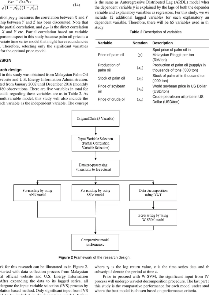
Figure 2 Framework of the research design. The framework for this research can be illustrated as in Figure 2.

This research is started with data collection process from Malaysian Palm Oil Council official website and U.S. Energy Information Administration. After expanding the data to its lagged series, all variables then undergone the input variable selection (IVS) process by using partial correlation based method. Only significant input from IVS will be considered to be included in the forecasting model. Before proceeding with the modelling process, the data series then have to be transformed to log return series (normalize). Because of the nature of most economic time series data that suffer from non-stationary condition, data transformation is needed. It is specified as below:

𝑟𝑡= log (

𝑧𝑡

𝑧𝑡−1) (15)

where 𝑟𝑡 is the log return value, 𝑧 is the time series data and the

subscript 𝑡 denote the period at time 𝑡.

Prior to proceed with W-SVM, the significant input from IVS process will undergo wavelet decomposition procedure. The last part of this study is the comparative performance for each model under study where the best model is chosen based on performance criteria.

Performance criteria

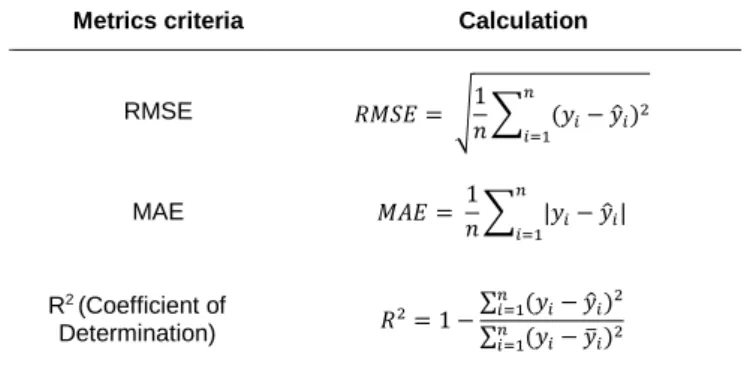
The prediction performance is evaluated using the following statistical metrics, namely, the root mean squared error (RMSE), mean absolute error (MAE) and coefficient of determination R2_{. The}

Table 3 Table of performance criteria. Metrics criteria Calculation

RMSE 𝑅𝑀𝑆𝐸 = √1 𝑛∑ (𝑦𝑖− 𝑦̂𝑖)2 𝑛 𝑖=1 MAE 𝑀𝐴𝐸 = 1 𝑛∑ |𝑦𝑖− 𝑦̂𝑖| 𝑛 𝑖=1 R2 _{(Coefficient of} Determination) 𝑅 2_{= 1 −}∑ (𝑦𝑛𝑖=1 𝑖− 𝑦̂𝑖)2 ∑ (𝑦𝑛𝑖=1 𝑖− 𝑦̅𝑖)2

RESULT AND DISCUSSION Data transformation

From Figure 3(a), the original data series shows nonstationary condition throughout the period of time. Forecasting under this condition might cause non-reliable result due to unstable variance in the data series. According to Lütkepohl & Xu (2009), a more stable variance series can result in dramatic gains in forecast precision. Therefore, data were transformed by using log return formula as in (15). The other advantage of using log return instead of normal log is the normalization of data series; which means that the variables are measured in comparable metric. After the transformation to log return series, monthly data price now become stationary as inFigure 3(b). This stationarity condition is important to give a better model accuracy.

Partial correlation based variable selection

As mentioned earlier, input variable selection is one of the important aspects in finding the optimal forecasting model. The partial correlation coefficient (𝜌) between the target variable and the input variable matrix is computed to determine the strength of their relationship. 1,000 1,500 2,000 2,500 3,000 3,500 4,000 02 03 04 05 06 07 08 09 10 11 12 13 14 15 16 Monthly Palm Oil Price

(a) -.16 -.12 -.08 -.04 .00 .04 .08 02 03 04 05 06 07 08 09 10 11 12 13 14 15 16 Monthly Palm Oil Price (Log Return)

(b)

Figure 3 Monthly price data (a) and the log return on monthly price data (b).

From the partial correlation coefficient matrix, p-value was computed for linear and rank partial correlations using a Student's t distribution for a transformation of the correlation. This p-value is for testing the hypothesis of no partial correlation against the one or two-sided alternative that there is a nonzero partial correlation. The Results show that from total of 64 variables, only 9 were significant and would be used as the inputs for our forecasting models. Table 4 shows the significant variables based on the partial correlation variable selection. Table 4 Significant variables based on partial correlation matrix.

Variable 𝝆 p-value x3t 0.5888 0.0000 yt-1 0.6436 0.0000 x2t-1 -0.2229 0.0157 x3t-1 -0.2468 0.0073 x1t-2 0.2378 0.0098 x2t-2 0.2039 0.0274 x1t-3 -0.1952 0.0349 x4t-3 -0.2479 0.0071 x4t-9 -0.1836 0.0475

Support vector machine regression

In this section, there are two main types of model that being studied; first is the SVM model by using normal data input and the second type is SVM model by using wavelet data input. This study will utilize three types of kernel function for SVM model that is; Linear, Gaussian (RBF) and Polynomial. They are differed according to mapping behavior to higher dimensional feature space. The advantage of linear kernel SVM is that it has only one parameter to tune that is the penalty C unlike RBF (Gaussian) and polynomial kernel, but Drucker, Wu, & Vapnik, (1999) concluded that upper bound C on coefficient αi affects the prediction performance if the data is not separable by a linear SVM. On the other hand, modelling of nonlinear SVM (RBF and polynomial) requires additional parameter to tune that is; γ for RBF kernel and, γ and degree d for polynomial kernel. Both kernels can handle nonlinear relation between the class label and its attribute. The optimum value of parameter C and γ are not known beforehand, therefore a parameter search must be employed. As suggested by Hsu, Chang, & Lin (2008), this study started SVM modeling by using RBF kernel to search for best parameter C and γ. This study conducts grid search using 5-fold cross validation to optimize the parameter C and γ for our problem. The grid range for both parameters is between a log-scaled of 1e-3 _{to 1e}3_{. There}

are 1000 combination of C and γ tested and the best pair is determined by the lowest value of cross-validation loss (error). Cross-validation loss (C-V loss) is the mean squared error between the observations in a fold when compared against predictions made on the out-of-fold data. The optimal value for C and γ based on the grid search are 1000 and 10 respectively with the cross-validation loss of 0.0023176. Table 5 shows the top ten result of grid search using 5-fold cross validation.

Table 5 Result for grid search using 5-fold cross validation

Rank C 𝜸 C-V loss 1 1000 10 0.0023176 2 215.44 10 0.0023207 3 215.44 10 0.0023216 4 215.44 10 0.0023363 5 215.44 10 0.0023420 6 1000 10 0.0023432 7 215.44 10 0.0023438 8 1000 10 0.0023566 9 1000 10 0.0023567 10 1000 10 0.0023603

Table 6 Result of SVM and wavelet SVM. The optimum parameter and performance of SVM model

Kernel C 𝜸 d RMSE MAE R2

Linear 1000 NA NA 110.6 86.82 0.8474

RBF 1000 10 NA 113.5 89.78 0.8393

Polynomial 1000 10 3 114.4 89.80 0.8366

Table 7 Forecasting performance for different wavelet functions at different decomposition level.

Decomposition level Performance

Wavelet function

Haar Daubechies Symlet

1 RMSE 130.60 100.10 86.08 MAE 82.11 69.99 67.48 R2 _{0.79 0.87 0.91} 2 RMSE 144.10 109.40 79.39 MAE 94.07 78.54 65.62 R2 _{0.74 0.85 0.92} 3 RMSE 149.80 101.40 81.84 MAE 100.50 71.57 65.56 R2 _{0.72 0.87 0.92} 4 RMSE 159.50 107.10 89.32 MAE 110.70 76.45 69.24 R2 _{0.68 0.86 0.90} 5 RMSE 155.40 114.50 87.52 MAE 112.00 75.63 68.61 R2 _{0.70 0.84 0.90} 6 RMSE 164.00 118.90 97.71 MAE 114.20 80.87 70.91 R2 _{0.66 0.82 0.88} 7 RMSE 163.30 110.30 97.36 MAE 113.50 75.36 72.20 R2 _{0.67 0.85 0.88}

Table 8 Summary of ANN model. Hidden

Neuron RMSE MAE R

2 Hidden

Neuron RMSE MAE R

2 1 119.36 99.66 0.82 ₁₁ 203.58 153.67 0.46 2 120.26 96.39 0.82 12 241.68 165.54 0.18 3 128.44 101.82 0.79 13 231.88 162.42 0.28 4 161.92 113.50 0.59 14 227.29 162.99 0.31 5 138.42 112.61 0.76 15 198.72 148.91 0.49 6 150.49 124.19 0.71 16 207.30 154.21 0.44 7 158.51 125.40 0.69 17 194.68 146.61 0.51 8 176.69 132.55 0.59 18 214.14 158.28 0.41 9 247.23 161.26 0.11 19 197.08 151.37 0.51 10 224.93 157.03 0.31

By using the optimal parameter from the grid search, training data was trained again to produce the final model. To determine which kernels generate the best model, this study performed SVM by using all-mentioned kernel (linear, RBF and polynomial). The performance of three different kernel functions as in Table 6.

Based on the result, model that uses polynomial kernel as the mapping function performs poorly compared to the other kernel with the RMSE, MAE and R2 of 114.4, 89.8 and 0.8366 respectively. Result for RBF kernel also shows the errors were almost the same as polynomial kernel with RMSE of 113.5, MAE equal to 89.78 and the R2 of .8393. The result also reveals that SVM with linear kernel generates the best model in term of error measurement with RMSE, MAE and R2 of 110.6, 86.82 and 0.8474 respectively.

Wavelet support vector machine (W-SVM)

Time series data obtained from partial correlation variable selection are decomposed into several sub-series components, then the optimal model from classical SVM is used to generate the model of W-SVM. Discrete wavelet transforms decomposed data series into two sets; approximation series and details series. Both of these series present better behavior that is in term of variance that more stable and there will be no outlier in the new series resulting from filtering effect of wavelet transform (Al Wadi et al., 2011).

This study utilized three most common types of wavelet function or family in time series analysis, that are; Haar, Daubechies and Symlet. In wavelet analysis, we also need to determine the decomposition level for our data. According to Yang, Sang, Liu, & Wang (2016), the maximum decomposition level (𝑀) for a wavelet function can be calculated as: 𝑀 = 𝑙𝑜𝑔2 (𝑁), where 𝑁 is the series length. Thus, the

maximum decomposition level for our study is 𝑙𝑜𝑔2 (180) ≈ 7; which

mean that the maximum number of different frequency of original series is 7, with an approximation component (A). For the purpose of this study, we perform all mentioned wavelet function with different decomposition level from 1 to 7 in order to determine the optimal wavelet function for our problem. The accuracy of optimal wavelet functions was compared according to the RMSE, MAE and R2 _{as in} Table 7.

Based on variable selection from partial correlation result, nine variables were used as the input data for W-SVM. For the purposes of comparative forecasting accuracy with previous SVM model, W-SVM model were trained as the same as normal SVM in previous section by using the best kernel in SVM that is linear with the same parameter C. The only exception is that all nine parameters were decomposed by using DWT. 21 models evaluated in W-SVM according to their wavelet function and decomposition level. From Table 7, the best forecasting accuracy according to performance criterion is from Symlet wavelet function at 2 level of decomposition with RMSE, MAE and R2 _{of 79.39,} 65.62 and 0.92 respectively.

By comparing the best model for W-SVM and SVM, there was significant increase in the forecasting accuracy where W-SVM model reduced the RMSE and MAE by 28.3%and 24.4%, and the coefficient of determination R2 _{improved by 8.8%. Theoretically, wavelet function} will improve the accuracy of forecasting performance, but note that some of the W-SVM models perform worse than normal SVM model such as for Haar wavelet function and wavelet functions that have more than four decomposition level. The result for Haar wavelet function is expected, because as discussed earlier, Haar wavelet is not appropriate in dealing with smooth function because it only has one vanishing moment. By comparing the performance of Daubechies and Symlet wavelet, the empirical result shows that Symlet function outperform Daubechies wavelet function. This is maybe due to the data structure that is asymmetric in nature. With that, the decomposition by using Symlet function will be more accurate compared to Daubechies function. Based on our result, the choice of wavelet function and decomposition level plays significant role in improving forecasting performance of SVM model.

Artificial neural network

In this study, input variable for ANN model was chosen based on the variable selection from partial correlation. In the early stage of data preparation, normalization process had been performed to the data. This process is important in ANN modelling to improve the network modeling and reducing the chances of being trapped in local minima.

For the network architecture, standard three-layer feed forward network is used in this study; with an input layer, a hidden layer and an output layer. In the input layer, nine nodes used represent the number of variables that being studied and for output layer, one node represents the response variable that is the price of palm oil. According to Shabri and Samsudin, (2014) one hidden layer is sufficient enough for ANN to approximate the complex nonlinear function with desired accuracy.

There are many practical guidelines from previous research in setting the optimal number of optimal number of hidden neuron in the hidden layer such as in Lippmann, (1987), Z. Tang & Fishwick (1993), Wong (1991) that was ranging from 1, n, 2n and 2n +1; where n is the number of input. However, there is no single best technique to determine the number of nodes in the hidden layer. Therefore, this study determined the best network architecture by trial and error from 1 neuron to 2𝑛 + 1 neurons for the hidden layer. This study employed Levenberg-Marquat algorithm provided by MATLAB to train the network. The maximum number of epochs was set at 1000 and each network was trained with different initial weights that were initialized randomly by using built-in MATLAB function. For each model, experiments were repeated 10 times and the average number of error measurement is calculated. This is to make sure that the result of each model is fair enough to represent the model without any bias. The summary of error measurement for ANN model is as in Table 8.

Based on the Table 8, the performance of ANN model is varying from 119.36 to 241.68 and 96.39 to 165.54 for RMSE and MAE respectively. The best ANN model architecture according to RMSE and MAE criterion has 9 input variables, 2 neurons in the hidden layer and 1 output layer neuron (9-2-1). The RMSE and MAE and R2 _{for this}

architecture are 120.26, 96.39 and 0.82 respectively.

CONCLUSION

This study considers three different approaches in forecasting palm oil price by using multivariate time series data. In the first model, classical SVM approach was used to model palm oil price series with its determinants. In the second model, the SVM approach was combined with wavelet decomposition method to develop a hybrid model for modelling palm oil price data series. The last model is the ANN approach used as the benchmark model to compare the performance of classical SVM and the hybrid W-SVM. There is additional preprocessing stage in the early part of the methodology where this study utilized partial correlation based variable selection to select the significant input to the model. The performances of all models were summarized in term of their accuracy as in Table 9.

Table 9 Performance of all models.

Model RMSE MAE R2

SVM 110.6 86.82 0.85

W-SVM 79.39 65.62 0.92

ANN 120.26 96.39 0.82

Based on the comparative performance of all models in Table 9, W-SVM model showed a significant improvement compared to the classical SVM (error reduced by 28% for RMSE and 24% for MAE) and outperformed ANN by 34% for RMSE and 32% for MAE in modelling palm oil price. The R2 _{for W-SVM also shows that the model}

fit better than classical SVM and ANN by 8% and 12% respectively. This study concluded that the wavelet decomposition technique plays a significant role in improving the forecasting ability of SVM model. However, based on the result of W-SVM, this improvement is subject to the selection of wavelet families that had been used. In SVM model,

input vectors were mapped into higher dimensional feature space by using three different kernels. Although Gaussian (RBF) kernel shows significant success in previous research, we found out that linear kernel is more suitable in our case. This is mostly due to the data structure that is linearly separable.

REFERENCES

Abdullah, R., & Lazim, M. A. (2006). Production and price forecast for malaysian palm oil. Oil Palm Industry Economic Journal, 6(1), 39–45. Abedinia, O., Amjady, N., & Zareipour, H. (2016). A new feature selection

technique for load and price forecast of electrical power systems. IEEE Transactions on Power Systems, 32(1), 62-74. https://doi.org/10.1109/ TPWRS.2016.2556620

Ahmad, M. H., Ping, P. Y., & Mahamed, N. (2014). Volatility modelling and forecasting of Malaysian crude palm oil prices. Applied Mathematical Sciences, 8(121–124), 6159–6169. https://doi.org/10.12988/ams.2014. 48650

Al Wadi, S., Ismail, M. T., Alkhahazaleh, M. H., & Karim, S. A. A. (2011). Selecting wavelet transforms model in forecasting financial time series data based on ARIMA Model. Applied Mathematical Sciences, 5(7), 315– 326. Retrieved from http://m-hikari.com/ams/ams-2011/ams-5-8-2011/alwadiAMS5-8-2011.pdf

Arshad, F. M., & Ghaffar, R. A. (1986). Crude Palm Oil Price Forecasting: Box-Jenkins Approach, Pertanika,9(3), 359–367.

Assis, K., Amran, A., Remali, Y., & Affendy, H. (2010). A comparison of univariate time series methods for forecasting cocoa bean prices. Trends in Agricultural Economics. Retrieved from http://www.researchersworld. com/vol1/Paper_7.pdf

Chen, B.-J., Chang, M.-W., & Lin, C.-J. (2004). Load forecasting using support vector machines: A study on EUNITE Competition 2001. IEEE Transactions on Power Systems, 19(4), 1821–1830. https://doi.org/ 10.1109/TPWRS.2004.835679

Deo, R. C., Wen, X., & Qi, F. (2016). A wavelet-coupled support vector machine model for forecasting global incident solar radiation using limited meteorological dataset. Applied Energy, 168, 568–593. https://doi.org/ 10.1016/j.apenergy.2016.01.130

Drucker, H., Burges, C. J. C., Kaufman, L., Smola, A., & Vapnik, V. (1997). Support vector regression machines. Advances in Neural Information Processing Systems, 1, 155–161. https://doi.org/10.1.1.10.4845

Drucker, H., Wu, D., & Vapnik, V. N. (1999). Support vector machines for spam categorization. IEEE Transactions on Neural Networks, 10(5), 1048– 1054. https://doi.org/10.1109/72.788645

Eynard, J., Grieu, S., & Polit, M. (2011). Wavelet-based multi-resolution analysis and artificial neural networks for forecasting temperature and thermal power consumption. Engineering Applications of Artificial Intelligence, 24(3), 501–516. https://doi.org/10.1016/j.engappai. 2010.09.003

Gençay, R., Whitcher, B., & Selçuk, F. (2002). An Introduction to Wavelets and other Filtering Methods in Finance and Economics. San Diego, California, USA: Academic Press.

Hamid, M. H., & Shabri, A. (2017). Wavelet regression model in forecasting crude oil price, AIP Conference Proceedings, 1842, 030019. https://doi.org/10.1063/1.4982857

Hsieh, T.-J., Hsiao, H.-F., & Yeh, W.-C. (2011). Forecasting stock markets using wavelet transforms and recurrent neural networks: An integrated system based on artificial bee colony algorithm. Applied Soft Computing,

11(2), 2510–2525. https://doi.org/10.1016/j.asoc.2010.09.007

Hsu, C.-W., Chang, C.-C., & Lin, C.-J. (2003). A practical guide to support vector classification. 1–16.

Jammazi, R., Lahiani, A., & Nguyen, D. K. (2015). A wavelet-based nonlinear ARDL model for assessing the exchange rate pass-through to crude oil prices. Journal of International Financial Markets, Institutions and Money, 34, 173–187. https://doi.org/10.1016/j.intfin.2014.11.011 Karia, A. A., Bujang, I., & Ahmad, I. (2013). Forecasting crude palm oil prices

using artificial intelligence approach. American Journal of Operatins Research, 3(2013), 259–267.

Khamis, A., & Wahab, N. A. (2016). Comparative study on predicting crude palm oil prices using regression and neural network models,International Journal of Science and Technology, 5(3), 88–94.

Khandelwal, I., Adhikari, R., & Verma, G. (2015). Time series forecasting using hybrid ARIMA and ANN models based on DWT decomposition. Procedia Computer Science, 48, 173–179. https://doi.org/10.1016/j.procs. 2015.04.167

Khin, A. A., Mohamed, Z., Malarvizhi, C. A. N., & Thambiah, S. (2013). Price forecasting methodology of the Malaysian palm oil market. The Internation Journal of Applied Economics and Finance, 7(1), 23–36. https://doi.org/10.3923/ijaef.2013.23.36

Kim, K.-J. (2003). Financial time series forecasting using support vector machines, Neurocomputing, 55(1-2), 307–319. https://doi.org/10.1016/ S0925-2312(03)00372-2

Kisi, O., & Cimen, M. (2011). A wavelet-support vector machine conjunction model for monthly streamflow forecasting. Journal of Hydrology, 399(1– 2), 132–140. https://doi.org/10.1016/j.jhydrol.2010.12.041

Lippmann, R. (1987). An introduction to computing with neural nets. IEEE ASSP Magazine, (April), 4(2) 4-22. https://doi.org/ 10.1109/MASSP.1987.1165576

Liu, F., & Fan, M. (2006). A hybrid support vector machines and discrete wavelet transform model in futures price forecastingIn: Wang J., Yi Z., Zurada J.M., Lu BL., Yin H. (eds) Advances in Neural Networks - ISNN 2006. ISNN 2006. Lecture Notes in Computer Science, vol 3973. Springer, Berlin, Heidelberg. https://doi.org/10.1007/11760191_71

Liu, X., Zhu, Y., Zhang, Y., & Wang, X. (2011). Prediction based on wavelet transform and support, In: Liu C., Chang J., Yang A. (eds) Information Computing and Applications. ICICA 2011. Communications in Computer and Information Science, vol. 243. Springer, Berlin, Heidelberg. https://doi.org/10.1007/978-3-642-27503-6_85

Lütkepohl, H., & Xu, F. (2009). The role of the log transformation in forecasting economic variables. Empirical Economics, 42(3), 619-638.

Mallat, S. (1989). A theory for multiresolution signal decomposition: the wavelet representation. IEEE Transactions on Pattern Analysis and Machine Intelligence,11(7), 674–693. https://doi.org/10.1109/ 34.192463 May, R., Dandy, G., & Maier, H. (2011). Review of input variable selection methods for artificial neural networks. In: Suzuki, K. (ed.), Artificial Neural Networks - Methodological Advances and Biomedical Applications, InTech. https://doi.org/10.5772/644

Min, J. H., & Lee, Y. (2005). Bankruptcy prediction using support vector machine with optimal choice of kernel function parameters, Expert Systems with Applications, 28(4), 603–614. https://doi.org/10.1016/j.eswa. 2004.12.008

Nochai, R., & Nochai, T. (2006). ARIMA Model for forecasting oil.

Proceedings of the 2nd IMT-GT Regional Conference on Mathematics, Statistics and Application, Penang, Malaysia, 13-15. Retrieved from http://web.vu.lt/ef/v.karpuskiene/files/2015/10/Arima-Palm-OIL-Price.pdf

Noori, R., Khakpour, A., Omidvar, B., & Farokhnia, A. (2010). Comparison of ANN and principal component analysis-multivariate linear regression models for predicting the river flow based on developed discrepancy ratio statistic. Expert Systems with Applications, 37(8), 5856–5862. https://doi.org/10.1016/j.eswa.2010.02.020

Nor, A. H. S. M., Sarmidi, T., & Hosseinidoust, E. (2014). Forecasting of palm oil price in Malaysia using linear and nonlinear methods, AIP Conference Proceedings 1613(1), 138–152. https://doi.org/10.1063/1.4894340 Ramesh, B. N., & Arulmozhivarman, P. (2013). Improving forecast accuracy of

wind speed using wavelet transform and neural networks. Journal of Electrical Engineering and Technology, 8(3), 559–564. https://doi.org/10.5370/JEET.2013.8.3.559

Rumelhart, D. E., McClelland, J. L., & PDP Research Group. (1986). Parallel distributed processing: Explorations in the microstructure cognition.

Psychological and biological models. Cambridge: MIT Press.

Shabri, A., & Samsudin, R. (2014). Daily crude oil price forecasting using hybridizing wavelet and artificial neural network model, Mathematical Problems in Engineering, 2014, Article No. 201402. http://dx.doi.org/ 10.1155/2014/201402

Shamsudin, M. N., & Arshad, F. M. (1999). Short term forecasting of Malaysian crude palm oil prices, 1–12. Retrieved from http://econ.upm.edu.my/ ~fatimah/pipoc.html

Shamsudin, M. N., Mohamed, Z. A., & Arshad, F. M. (1988). Selected factors affecting palm oil price. Malaysian Journal of Agriculture Economics, 5, 20–29.

Stolojescu, C., Railean, I., Moga, S., & Isar, A. (2010). Comparison of wavelet families with application to WiMAX traffic forecasting. Proceedings of the International Conference on Optimisation of Electrical and Electronic Equipment, OPTIM, 932–937. https://doi.org/10.1109/OPTIM.2010. 5510403

Tang, L. B., Tang, L. X., & Sheng, H. Y. (2009). Forecasting volatility based on wavelet support vector machine. Expert Systems with Applications, 36(2 PART 2), 2901–2909. https://doi.org/10.1016/j.eswa.2008.01.047 Tang, Z., & Fishwick, P. A. (1993). Feedforward neural nets as models for time

series forecasting. INFORMS Journal on Computing, 5(4), 374–385. https://doi.org/10.1287/ijoc.5.4.374

Tay, F. E. H., & Cao, L. (2001). Application of support vector machines in ÿnancial time series forecasting, Omega 29(4), 309–317.

Wong, F. S. (1991). Time series forecasting using backpropagation neural networks. Neurocomputing, 2(4), 147–159. https://doi.org/10.1016/0925-2312(91)90045-D

vector regression. IEEE Transactions on Intelligent Transportation Systems, 5(4), 276–281. https://doi.org/10.1109/TITS.2004.837813 Yang, M., Sang, Y. F., Liu, C., & Wang, Z. (2016). Discussion on the choice of

decomposition level for wavelet based hydrological time series modeling.

Water (Switzerland), 8(5), 1–11. https://doi.org/ 10.3390/w8050197 Zhang, G., Eddy Patuwo, B., & Y. Hu, M. (1998). Forecasting with artificial

neural networks: The state of the art. International Journal of Forecasting,