c
SELECTIVE ALGORITHMS FOR LARGE-SCALE CLASSIFICATION AND STRUCTURED LEARNING
BY
KAI-WEI CHANG
DISSERTATION
Submitted in partial fulfillment of the requirements for the degree of Doctor of Philosophy in Computer Science
in the Graduate College of the
University of Illinois at Urbana-Champaign, 2015
Urbana, Illinois
Doctoral Committee:
Professor Dan Roth, Chair Professor David Forsyth Professor ChengXiang Zhai Doctor John Platt, Google
Abstract
The desired output in many machine learning tasks is a structured object, such as tree, clustering, or sequence. Learning accurate prediction models for such problems requires training on large amounts of data, making use of expressive features and performing global inference that simultaneously assigns values to all interrelated nodes in the structure. All these contribute to significant scalability problems. In this thesis, we describe a collection of results that address several aspects of these problems – by carefully selecting and caching samples, structures, or latent items.
Our results lead to efficient learning algorithms for large-scale binary classification models, structured prediction models and for online clustering models which, in turn, support reduction in problem size, improvements in training and evaluation speed and improved performance. We have used our algorithms to learn expressive models from large amounts of annotated data and achieve state-of-the art performance on several natural language processing tasks.
Publication Notes
Parts of the work in this thesis have appeared in the following publications:
• K.-W. Chang and D. Roth. Selective block minimization for faster convergence of limited memory large-scale linear models. InProc. of the ACM SIGKDD Conference on Knowledge Discovery and Data Mining (KDD), 2011.
• K.-W. Chang, R. Samdani, A. Rozovskaya, N. Rizzolo, M. Sammons, and D. Roth. Inference protocols for coreference resolution. In Proc. of the Conference on Computational Natural Language Learning (CoNLL) Shared Task, 2011.
• K.-W. Chang, R. Samdani, A. Rozovskaya, M. Sammons, and D. Roth. Illinois-coref: The UI system in the conll-2012 shared task. In Proc. of the Conference on Computational Natural Language Learning (CoNLL) Shared Task, 2012.
• K.-W. Chang, R. Samdani, and D. Roth. A constrained latent variable model for coreference resolution. InProc. of the Conference on Empirical Methods in Natural Language Processing (EMNLP), 2013.
• K.-W. Chang, V. Srikumar, and D. Roth. Multi-core structural svm training. In Proc. of the European Conference on Machine Learning and Principles and Practice of Knowledge Discovery in Databases (ECML PKDD), 2013.
• K.-W. Chang, S. Upadhyay, G. Kundu, and D. Roth. Structural learning with amortized inference. InProceedings of the National Conference on Artificial Intelligence (AAAI), 2015.
Other relevant publications by the author:
• K.-W. Chang, A. Krishnamurthy, A. Agarwal, H. Daume III, J. Langford. Learning to Search Better Than Your Teacher. Arxiv:1502.02206 (preprint), 2015.
• K.-W. Chang, B. Deka, W.-M. W. Hwu, and D. Roth. Efficient pattern-based time series classification on GPU. In Proc. of the IEEE International Conference on Data Mining (ICDM), 2012.
• R. Samdani, K.-W. Chang, and D. Roth. A discriminative latent variable model for online clustering. In Proceedings of the International Conference on Machine Learning (ICML), 2014.
• K.-W. Chang, W.-t. Yih, B. Yang, and C. Meek. Typed tensor decomposition of knowledge bases for relation extraction. In Proceedings of the Conference on Empirical Methods for Natural Language Processing (EMNLP), 2014.
• K.-W. Chang, S. Sundararajan, S. S. Keerthi, and S. Sellamanickam. Tractable semi-supervised learning of complex structured prediction models. InProceedings of the European Conference on Machine Learning (ECML), 2013.
• H.-F. Yu, C.-J. Hsieh, K.-W. Chang, and C.-J. Lin. Large linear classification when data cannot fit in memory. In Proceedings of International Conference on Knowledge Discovery and Data Mining (KDD), 2010.
• C.-J. Hsieh, K.-W. Chang, C.-J. Lin, S. S. Keerthi, and S. Sundararajan. A dual coordinate descent method for large-scale linear svm. InProceedings of the International Conference on Machine Learning (ICML), 2008.
Acknowledgments
I would like to express my sincere thanks to my advisor, Prof. Dan Roth, for his guidance and tremendous support over the past five years. Dan is not only a remarkable scholar but also a passionate educator. His foresight in research, his dedication to mentoring, and his open-minded personality have greatly influenced me. He has demonstrated what it means to be a great advisor. I was fortunate to have David Forsyth, ChengXiang Zhai, and John Platt on my dissertation committee, from which I got valuable and constructive comments. I am lucky to have worked with and to have been mentored by John Langford, Hal Daum’e III, Alekh Agrawal, Scott Yih, Chris Meek, Sathiya Keerthi, and Sundararajan Sellamanickam during my internship. I benefited greatly from discussions with them. I am also thankful to my former advisor, Chih-Jen Lin, who equipped me with solid research skills.
In addition, I would like to acknowledge Ming-Wei Chang, Vivek Srikumar, and Rajhans Sam-dani for supporting me in the early stage of my Ph.D. studies. They always patiently answered my many questions. Mark Sammons taught me many things and has been always supportive. Eric Horn also assisted me in many aspects, especially in job finding. Nick Rizzolo, Alla Ro-zovskaya, Biplab Deka, Shyam Upadhyay, Lev Ratinov, He He, Akshay Krishnamurthy, Gourab Kundu, Haoruo Peng, Chen-Tse Tsai, and Ching-Pei Lee were collaborators in many of my projects, and I learned a lot from discussions with them. I would also like to thank my colleagues in the CogComp group, including Quang Do, Prateek Jindal, Jeff Pasternack, Dan Goldwasser, Parisa Kordjamshidi, Daniel Khasabi, Wei Lu, Stephen Mayhew, Subhro Roy, Yangqiu Song, Yuancheng Tu, Vinod Vydiswaran, John Weiting and Christos Christodoupoulos. Many thanks to all my friends from Taiwanese community in Champaign-Urbana for making my life colorful.
Table of Contents
List of Tables . . . ix
List of Figures . . . xi
List of Abbreviations . . . xiii
Chapter 1 Introduction . . . 1
1.1 Motivating Examples and Challenges . . . 3
1.1.1 Large-Scale Classification . . . 3
1.1.2 Supervised Clustering: Coreference Resolution . . . 4
1.2 Selective Algorithms for Learning at Scale . . . 5
1.3 Overview of This Work . . . 6
Chapter 2 Background . . . 9
2.1 Binary Classification . . . 10
2.1.1 Linear Support Vector Machines . . . 11
2.2 Structured Prediction . . . 12
2.2.1 Inference for Structured Models . . . 14
2.2.2 Learning Structured Prediction Models . . . 15
Chapter 3 Training Large-scale Linear Models With Limited Memory . . . 20
3.1 A Selective Block Minimization Algorithm . . . 21
3.2 Multi-class Classification . . . 25
3.3 Learning from Streaming Data . . . 26
3.4 Implementation Issues . . . 27
3.4.1 Storing Cached Samples in Memory . . . 28
3.4.2 Dealing with a Largeα . . . 28
3.5 Related Work . . . 29
3.6 Experiments . . . 31
3.6.1 Training Time and Test Accuracy . . . 32
3.6.2 Experiments on Streaming Data . . . 37
3.6.3 Experiments Under The Single Precision Floating Point Arithmetic . . . 39
3.6.4 Cache Size . . . 40
Chapter 4 Multi-core Structural SVM Training . . . 42
4.1 A Parallel Algorithm for Training Structural SVM Models . . . 43
4.1.1 Analysis . . . 46
4.2 Related Work . . . 47
4.3 Experiments . . . 49
4.3.1 Experimental Setup . . . 49
4.3.2 Empirical Convergence Speed . . . 51
4.3.3 CPU Utilization . . . 52
4.3.4 Performance with Different Number of Threads . . . 54
4.4 Conclusion . . . 54
Chapter 5 Amortized Inference for Structured Prediction . . . 56
5.1 Amortized Inference . . . 58
5.1.1 Exact Amortized Inference Theorems . . . 59
5.1.2 Approximate Amortized Inference Theorems . . . 61
5.2 Learning with Amortized Inference . . . 62
5.2.1 Structured SVM with Amortized Inference . . . 63
5.2.2 Structured Perceptron with Amortized Inference . . . 65
5.3 Experiments and Results . . . 66
5.3.1 Learning with Amortized Inference . . . 67
5.3.2 Cross Validation using Amortization . . . 70
5.4 Conclusion . . . 71
Chapter 6 Supervised Clustering on Steaming Data . . . 72
6.1 Coreference Resolution . . . 72
6.2 Pairwise Mention Scoring . . . 74
6.2.1 Best-Link . . . 75
6.2.2 All-Link . . . 77
6.3 Latent Left-Linking Model . . . 78
6.3.1 Learning . . . 79
6.3.2 Incorporating Constraints . . . 80
6.4 Probabilistic Latent Left-Linking Model . . . 82
6.5 Related Work . . . 84
6.6 Experiments . . . 86
6.6.1 Experimental Setup . . . 86
6.6.2 Performance of the End-to-End System . . . 88
6.6.3 Analysis on Gold Mentions . . . 90
6.6.4 Ablation Study of Constraints . . . 92
6.7 Conclusion . . . 92
Chapter 7 Conclusion and Discussion . . . 94
References . . . 97
Appendix A Proofs . . . 107
A.1 Proof of Theorem 1 . . . 107
List of Tables
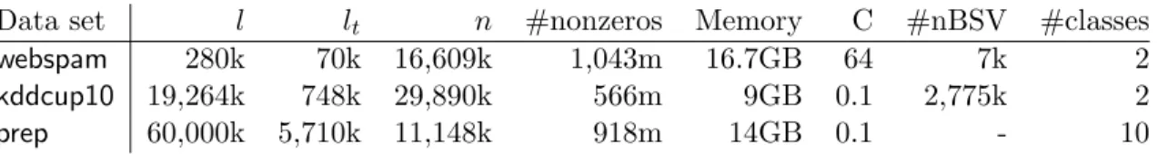
2.1 Notation. . . 10 3.1 Data statistics: We assume the data is stored in a sparse representation. Each
feature with non-zero value takes 16 bytes on a 64-bit machine due to data structure alignment. l, n, and #nonzeros are numbers of instances, features, and non-zero values in each training set, respectively. ltis the number of instances in the test set. Memory is the memory consumption needed to store the entire data. #nBSV shows the number of unbounded support vectors (0 < αi < C) in the optimal solution. #classes is the number of class labels. . . 32 3.2 Training time (wall clock time) and test accuracy for each solver when each sample
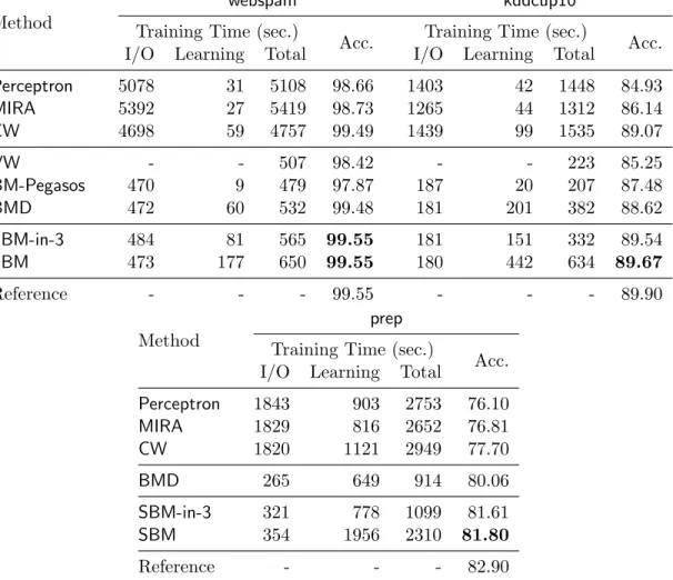
is loaded into memory only once. We show both the loading time (the time to read data from an ASCII file) and the learning time. The reference model is obtained by solving (2.4) until it converges (see text). We show that by updating the model on one data block at a time, SBM obtains an accurate model for streaming data. Note that the time reported here is different from the time required to finish the first iteration in Figure 3.1 (see text). Some entries in the table are missing. BM-Pegasos and VW do not support multi-class classification. Also, it is difficult to access the I/O and learning time of VW since it is a multi-threaded program. The top three methods are implemented in Java, and the rest are in C/C++. . . 37 5.1 Ratio of inference engine calls, inference time, inference speedup, final negative dual
objective function value (−D(α) in Eq. (2.14)) and the test performance of each method. Time is in seconds. The results show that AI-DCD significantly speeds up the inference during training, while maintaining the quality of the solution. Remark-ably, it requires 24% of the inference calls and 55% of the inference time to obtain an exact learning model. The reduction of time is implementation specific. . . 67 6.1 Performance on OntoNotes-5.0 with predicted mentions. We report the F1 scores
(%) on various coreference metrics (MUC, BCUB, CEAF). The column AVG shows the averaged scores of the three. The proposed model (CL3M) outperforms all the others. However, we observe that PL3M and CPL3M (see Sec. 6.4) yields the same performance as L3M and CL3M, respectively as the tuned γ for all the datasets turned out to be 0. . . 88 6.2 Performance on named entities for OntoNotes-5.0 data. We compare our system to
6.3 Performance on ACE 2004 and OntoNotes-5.0. All-Link-Red. is based on correla-tional clustering; Spanning is based on latent spanning forest based clustering (see Sec. 6.5). Our proposed approach is L3M (Sec. 6.3) and PL3M (sec. 6.4). CL3M and CPL3M are the version with incorporating constraints. . . 91 6.4 Ablation study on constraints. Performance on OntoNotes-5.0 data with predicted
List of Figures
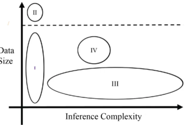
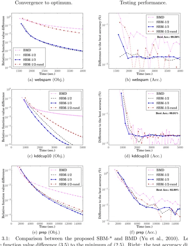
1.1 The size of the learning problems and the inference complexity of the model. This thesis focuses on the problems in regions II and III, though we will discuss an al-gorithm for learning latent representations of a knowledge base, where the learning problem is both large and complex (region IV). Prior work by the author of this thesis partly concerns problems in region I. The dashed line indicates a limitation on the size of the data that can be fully loaded into main memory, and where our region II is relative to it. . . 2 3.1 Comparison between the proposed SBM-* and BMD (Yu et al., 2010). Left: the
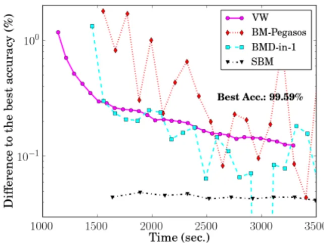
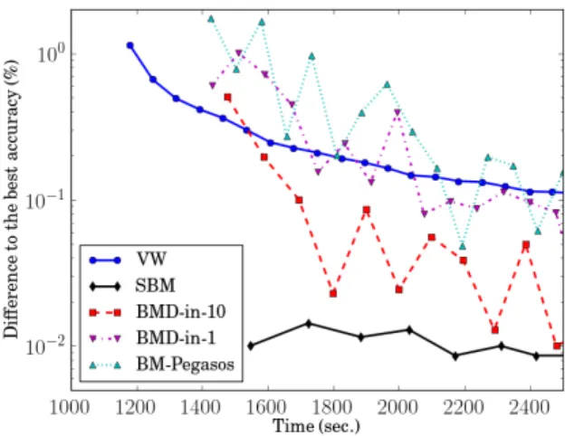
relative function value difference (3.5) to the minimum of (2.5). Right: the test accuracy difference (3.6) from the best achievable accuracy. Time is in seconds, and the y-axis is in log-scale. Each marker indicates one outer iteration. As all the solvers access all samples from disk once at each outer iteration, the markers indicate the amount of disk access. . . 34 3.2 A comparison between SBM and online learning algorithms on webspam. We show
the difference between test performance and the best accuracy achievable (3.6). Time is in seconds. The markers indicate the time it takes each solver to access data from disk once. Except for VW, each solver takes about 90 sec. in each round to load data from the compressed files. . . 36 3.3 A comparison among SBM, BMD and online learning algorithms on webspam. All
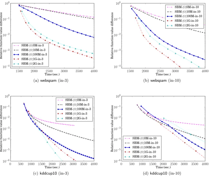
the methods are implemented with single precision. We show the difference between test performance and the best accuracy achievable (3.6). Time is in seconds. The markers indicate the time it takes each solver to access data from disk once. . . 39 3.4 The relative function value difference (3.5) to the optimum of (2.5). Time is in
seconds, and the y-axis is in log-scaled. We show the performance of SBM with various cache sizes. SBM-|Ω|0M-in-* is equivalent to BMD. We demonstrate both the situations that SBM solves the sub-problem with 3 rounds and 10 rounds. . . . 41 4.1 Relative primal function value difference to the reference model versus wall clock
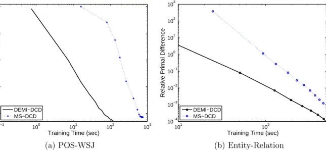
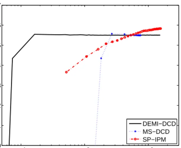
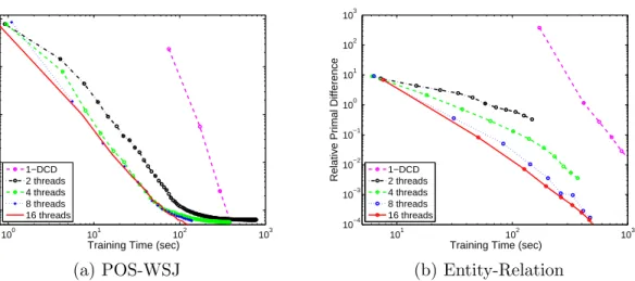
time. See the text for more details. . . 52 4.2 Performance of POS-WSJ and Entity-Relation plotted as a function of wall clock
training time. For Entity-Relation, we report the F1 scores of both entity and rela-tion tasks. Note that the X-axis is inlog scale. We see that DEMI-DCDconverges faster to better performing models. . . 53
4.3 CPU usage of each method during training. The numbers listed in the caption are the average CPU usage percentage per second for DEMI-DCD,MS-DCD,SP-IPM, respectively. We show moving averages of CPU usage with a window of 2 seconds. Note that we allow all three algorithms to use 16 threads in a 24 core machine. Thus, while all the algorithms can report upto 1600% CPU usage, only DEMI-DCD consistently reports high CPU usage. . . 54 4.4 Relative primal function value difference along training time using different number
of threads. We also show a DCD implementation using one CPU core (1-DCD). Both x-axis and y-axis are in log scale. . . 55 5.1 Left: The number of inference engine calls by a raw solver, an oracle solver and our
method when training a structured SVM model on an entity-relation recognition corpus. The raw solver calls an inference engine each time an inference is needed, while the oracle solver only calls the engine when the solution is different from all solutions observed previously. Our method significantly reduces the number of inference calls required to train a model. Right: Our models require less inference calls to reach a certain level of performance. . . 57
List of Abbreviations
ILP Integer Linear Programming NLP Natural Language Processing POS Part-of-Speech Tagging CRF Conditional Random Field SVM Support Vector Machine
SSVM Structured SVM
WSJ Wall Street Journal
BMD Block Minimization Algorithm SBM Selective Block Minimization L3M Latent Left-Linking Model
PL3M Probabilistic Latent Left-Linking Model DCD Dual Coordinate Descent
DEMI-DCD DEcoupled Model-update and Inference with Dual Coordinate Descent AI-DCD Amortized Inference framework for Dual Coordinate Descent
Chapter 1
Introduction
Machine learning techniques have been successfully applied in many fields, including natural lan-guage processing (NLP), computer vision, information retrieval, and data mining. Among these, classification methods and structured prediction models are two of the most widely used techniques. Standard classification methods are useful when a prediction problem can be formulated as one or several independent binary (True/False) or multiple-choice questions. Statistical learning tech-niques (e.g., support vector machine (Cortes and Vapnik, 1995) and logistic regression) have been widely studied for such problems. Many of these can be scaled up to handle relatively large amounts of data in applications like spam detection, object recognition, network intrusion detection, and human splice site recognition. On the other hand, many prediction problems consist of several inter-dependent binary or multiple-choice decisions. One can model the interrelated decision vari-ables involved in these problems using a structured object, such as linear chain, clustering, or tree. Theses types of models are known as structured prediction models and are typically expressed as probabilistic models over a set of variables (e.g., Bayesian networks (Pearl, 1988), Markov random fields (Kindermann and Snell, 1980), factor graphs (Kschischang et al., 2001), and constrained con-ditional models (Chang et al., 2012b)). To estimate the parameters involved in these models from annotated data, many approaches have been proposed, including decomposed learning (Heckerman et al., 2000; Samdani and Roth, 2012), max-margin learning (Taskar et al., 2004; Joachims et al., 2009), and constraint-driven learning (Chang et al., 2012b). To focus our discussion, this thesis focuses on supervised discriminative learning methods for classification and structured prediction models.
During the last decade, the size of data sets used to build classifiers and structured predictors has steadily increased. The availability of large amounts of annotated data (e.g., for web
applica-Figure 1.1: The size of the learning problems and the inference complexity of the model. This thesis focuses on the problems in regions II and III, though we will discuss an algorithm for learning latent representations of a knowledge base, where the learning problem is both large and complex (region IV). Prior work by the author of this thesis partly concerns problems in region I. The dashed line indicates a limitation on the size of the data that can be fully loaded into main memory, and where our region II is relative to it.
improving the quality of practical models, but also raise a scalability issue. Scalability is influenced by two key dimensions: the size of the data and the complexity of the decision structures. If the data is too large, training even a simple binary classifier can be difficult. For example, Yu et al. (2010) demonstrated a failure to train a binary classifier using Liblinear (Fan et al., 2008), a pop-ular linear classification library, on a data set that was too large to be fully loaded into memory. When the data cannot fit into memory, batch learners, which load the entire data during the train-ing process, suffer severely due to disk swapptrain-ing (Yu et al., 2010). Even online learntrain-ing methods, which deal with the memory problem by loading a portion of data at each time step, take consid-erable number of iterations to converge to a good model. Consequently, they require significant amount of disk access which slows down the training process. And, complex dependencies among the variables of interests are to be modeled, it is essential to consider an expressive model which makes exact learning and inference time consuming. In extreme cases, inferences over complex decision structures are practically intractable. Even where the decision structure is tractable, the time complexity of a typical inference algorithm is super-linear in the size of the output variables. As a result, the inference procedure often becomes a bottleneck in the learning process. Figure 1.1 depicts the scale of the machine learning problems and the focus of the thesis.
This thesis develops a conceptually unified approach, Selective Learning Algorithms, and, within it, presents several efficient learning algorithms that address the dimensions of scalability discussed above – large data sets and expressive dependencies among variables of interest. These approaches are based on an observation that a machine learning algorithm often consists of manysmall oper-ations and sub-components. For example, when solving a binary classification problem with many training samples, one needs to update the model based on each sample. Each update takes a small amount of time, but in total, it contributes to the overall training time and, often, makes it much longer than possible or needed. Therefore, by identifying important components in the training process, we can devote more effort and resources (e.g., memory and computational power) to these selected components. We may even cache the computation on these components to save future computation, and, consequently, we may not need to attend to all components. This leads to a unified strategy that can be used to accelerate the training process.
In the rest of this chapter, we first present two motivating examples. Then, we provide more details about our approaches and contributions.
1.1
Motivating Examples and Challenges
In this section, we provide some examples that motivate the scalability issues in machine learning. 1.1.1 Large-Scale Classification
In the past few years, the size of data available for analysis has grown drastically. Many Internet companies report the need to learn on extremely large data sets, and consequently, benchmark data sets used by research increased significantly in size. For example, in one visual recognition challenge, ImageNet,1 the learning task requires handling a data set of hundreds of gigabytes. Google reports that they have data sets with a hundred billion instances.2 A learning task for recognizing a human acceptor splice (Sonnenburg and Franc, 2010) generates a dataset that requires 600 GB of memory to store. In some applications, unlimited amounts of annotated data can be generated. For example, we will show an example in Section 3.6 in which an infinite number of examples can be generated
1
http://www.image-net.org
in order to learn a predictor for correct prepositions. Bottou3 also shows that an infinite number of digit images can be generated from the MNIST dataset by pseudo-random deformations and translations (Loosli et al., 2007). All the above examples show the need for efficient and effective algorithms to handle large-scale data, and it has been argued that using more samples and adding more features (e.g, using n-gram in a bag-of-words model) actually boosts performance.
The challenge of training a model on large amounts of data is two-fold. First, as we mentioned above, although the computation involved in updating the model on each example is small, this accumulates, when dealing with large amounts of data, and becomes very significant. Second, when the data is large, memory access often becomes the bottleneck. The situation is even worse when the data is too large to fit in memory. In Chapter 3, we will show that by selecting informative instances during the training, we can significantly reduce the training cost on large-scale data. 1.1.2 Supervised Clustering: Coreference Resolution
Many machine learning applications, including spam filtering (Haider et al., 2007), network in-trusion detection (Guha et al., 2003), and thread detection in text messages (Shen et al., 2006), need to cluster items based on their similarity. Different from transitional unsupervised clustering problems, where evaluating clustering is often a key issue, the clusters in these clustering problems have clear semantics. Therefore it is possible to obtain supervised data, which can be used to train and evaluate the clustering models.
In the following, we use an NLP task as a motivating example to demonstrate the scalability problems. Consider the following paragraph and the question:
(ENGLAND, June, 1989) - [Christopher Robin] is alive and well. He lives in England. He is the same person that you read about in the book, Winnie the Pooh. As a boy, Chris lived in a pretty home called Cotchfield Farm. When [Chris] was three years old, his father wrote a poem about him. The poem was printed in a magazine for others to read. [Mr. Robin] then wrote a book. He made up a fairy tale land where Chris lived. His friends were animals. There was a bear called Winnie the Pooh. There was also an owl and a young pig, called a piglet. All the animals were stuffed toys that
3
Chris owned.
Q: Do [Christopher Robin], [Chris] and [Mr. Robin] (the boldfaced mentions) refer to the same person?
At the first glance, one might think that[Chris]and[Mr. Robin]both refer to[Christopher Robin]. However, after carefully reading the paragraph, we know that[Mr. Robin]refers to his fatherin the fourth line, andhisrefers to[Chris]. Therefore,[Mr. Robin]refers to Chris’s father and cannot be the same as[Chris]. This suggests that in order to correctly answer this question, we need to consider the complex decision structure, and simultaneously take several pairwise local decisions (e.g., does[Mr. Robin] refer to his father?) into account.
The general setting of this problem is calledcoreference resolution, where we want to group the noun phrases (mentions) into equivalence classes, so that the mentions in the same class refer to the same entity in the real world. For example, all the underlined mentions in the above paragraph refer to the same entity,Christopher Robin. Therefore, they belong to the same group. We consider a supervised learning setting, where we assume a collection of articles with coreference annotations. The goal is to learn a model that predicts the coreference clusters for a previously unseen document. A natural way to model this problem is to break the coreference clustering decision into pairwise local decisions, which estimate whether two mentions can be put into the same coreference cluster. As shown in the example above, these local predictions are mutually dependent and have to obey the property of transitivity. Therefore, the inference procedure requires global consideration of all assignments simultaneously, resulting in a computational difficulty. This is a typical scalability issue when dealing with problems having a complex structure. We will provide more details in Chapters 2 and 6.
1.2
Selective Algorithms for Learning at Scale
Various approaches have been proposed to train models on large and complex data. Most ap-proaches have focused on designing optimization methods (Joachims, 2006; Shalev-Shwartz et al., 2007; Taskar et al., 2005; Chang and Yih, 2013; Lacoste-Julien et al., 2013) and parallel algo-rithms (Woodsend and Gondzio, 2009; Chang et al., 2007a; Agarwal et al., 2014; McDonald et al.,
have been shown to be capable of handling large-scale data (Crammer et al., 2006; Dredze et al., 2008; Crammer et al., 2009; Collins, 2002) as well.
In this thesis, we will explore another orthogonal direction – saving computation by selecting important components, such as instances, candidate structures, and latent items, and devoting more effort to them during the training. The informative components can be predefined but are often selected by the model. We will demonstrate that this idea can be applied when designing efficient learning algorithms as well as when modeling problems involving complex decisions. In all cases, the training time is reduced without compromising the performance of the model. In some cases, the performance even improves (see Chapter 6). We will provide sound theoretical justifications of the selection framework. Specifically, from an optimization perspective, selecting informative samples and candidate structures can be treated as solving the learning problem using block coordinate descent in the dual form. From a modeling perspective, selecting latent items is related to the latent structured models (Quattoni et al., 2007; Yu and Joachims, 2009; Samdani et al., 2012b).
Some earlier approaches in the literature have similarities to some aspects of the approach presented in this thesis. Selecting informative components during the training has been discussed in the literature, such as working set selection and the shrinking strategy for kernel SVM (Keerthi et al., 2001; Fan et al., 2005; Joachims, 1999), caching for Perceptron (Collins and Roark, 2004), emphasizing scheme (Guyon et al., 1992), and selective sampling for training on large data (P´ erez-Cruz et al., 2004; Tong and Koller, 2002; Yu et al., 2003). Dual coordinate descent and sequential minimal optimization have been widely discussed especially for solving the SVM problem and its variants (e.g., (Platt, 1999; Hsieh et al., 2008; Shalev-Shwartz and Zhang, 2013)). We will provide more discussions in the related work section in each chapter.
1.3
Overview of This Work
This thesis addresses scalability problems, such as those discussed in previous sections. We derive efficient selective algorithms for three different scenarios:
• designing a parallel algorithm to select candidate structures while learning a structured model (Chapter 4) and
• selecting and caching inference solutions in learning a structured model (Chapter 5); and • selecting latent items for online clustering models (Chapter 6).
We provided a summary of our contributions below.
Learning with Large-Scale Data. In Chapter 3, we propose a selective block minimization
(SBM) framework (Chang and Roth, 2011) for data that cannot fit in memory. The solver loads and trains on one block of samples at a time and caches informative samples in memory during the training process. Thus, it requires fewer data loads before reaching a given level of performance relative to existing approaches. By placing more emphasis on learning from the data that is already in memory, the method enjoys provably fast global convergence and reduces training time, in some problems, from half a day to half an hour. It can even obtain a model that is as accurate as the optimal one with just a single pass over the data set. For the same data, the best previously published method (Yu et al., 2010) requires loading the data from disk 10 times to reach the same performance.
Learning and Inference for General Structured Prediction Models. In many cases,
deci-sion making involves predicting a set of interdependent outputs. Structured prediction models have been proposed to model these interdependencies, and have been shown to be powerful. However, their high computational cost often causes a scalability problem. In this thesis, we explore methods which select and cache candidate structures when learning structured prediction models. We show how to improve structured training algorithms from two orthogonal directions – parallelism and amortization.
In Chapter 4, we introduce the DEMI-DCDalgorithm (DEcoupled Model-update and Inference with Dual Coordinate Descent) (Chang et al., 2013b), a new barrier-free parallel algorithm based on the dual coordinate descent (DCD) method for the L2-loss structural SVM, which is a popular structured prediction model. DEMI-DCD removes the need for a barrier between a model update phase and an inference phase involved in the training, allowing us to distribute these two phases
methods, while maintaining sound convergence properties.
In Chapter 5, we observed that training a structured prediction model involves performing several inference steps. Over the lifetime of training, many of these inference problems, although different, share the same solution. We demonstrate that by exploiting this redundancy of solutions, a solver can reduce by 76% – 90% the number of inference calls needed without compromising the performance of the model, thus significantly reducing the overall training time (Chang et al., 2015).
Learning and Inference with a Highly Complex Structure. Many applications involve a
highly complex structure. In such situations, learning and inference are intractable. In Chapter 6, we show that the idea of selection can be used to model such a problem. Specifically, we design an auxiliary structure that simplifies a complex structured prediction model for on-line supervised clustering problems. For each item, the structure selects only one item (in this case, the one to its left in the mention sequence) and uses it to update the pairwise metric (a feature-based pairwise item similarity function), assuming a latent left linking model (L3M). We derive efficient learning and inference algorithms for L3M and apply them to the coreference resolution problem, which is aimed at clustering denotative phrases (“mentions”) that refer to the same entity into an equivalent class. This leads to an efficient and principled approach to the problem of on-line clustering of streaming data. In particular, when applied to the problem of coreference resolution, it provides a linguistically motivated approach to this important NLP problem (Chang et al., 2013a). This was the best performing coreference system at the time of publication, and the approach has become mainstream and inspired follow-up work (Ma et al., 2014; Lassalle and Denis, 2015).
Chapter 2
Background
Statistical machine learning approaches have been widely used in many applications, including predicting linguistic structure and semantic annotation. In this chapter, we briefly introduce the corresponding notation and the necessary background knowledge. We mainly focus on the general concepts used in classification and structured prediction, where training a model is time-consuming. Table 2.1 lists the notation used throughout this thesis. The goal of a machine learning al-gorithm is to learn a mapping function f(x;w) from an input space X to an output space Y. Depend on how a learning problem is modeled, the output variable of interest can be binary (i.e., y ∈ {1,−1}), categorical (y ∈ {1,2,3, . . . , k}), or structured ( y = (y1, y2, . . . , yj, . . . yk), where yj ∈ Yj, a discrete set of candidates for the output variable yj, and y∈ Y, a set of feasible struc-tures). This mapping function can be parameterized with weightswof task-relevant featuresφ(·). If the output variable is binary or categorical, the features are typically defined only on input, and can be represented as a feature vectorφ(x). For notational simplicity in this thesis, we usex instead of φ(x) to represent this feature vector. If the output variable is modeled as a structured object, the feature vector φ(x,y) is often defined on both input and output, allowing us to take into account the interdependency between variables in the structured object.
We assume there is an underlining distribution P(x,y) to the data. Unless stated otherwise, in a supervised learning setting, we assume that a set of independent and identically distributed (i.i.d.) training data D = (xi,yi)li=1 is given. The goal of supervised learning is to estimate the
mapping function using the training data, such that the expected loss is minimal:
E[f] =
Z
X ×Y
Notation Description D Dataset x∈Rn Input instance y ∈ {1,−1} Output (binary) y ∈ {1,2,3, . . . , k} Output (multiclass) y∈ Y Structured Output
φ(·) Feature generating function
w∈Rd Weight vector
∆(y0,y) Distance between structuresy0 Table 2.1: Notation.
output variable is binary or categorical, ∆ is usually defined as a zero-one loss,
∆(y, y0) =I(y6=y0), (2.2)
whereI(·) is an indicator function. If the output is structured, a common choice of the loss function is Hamming loss ∆(y,y0) =P
iI(yi6=y0i), whereyi is the sub-component ofy.
Once the mapping function is learned, we proceed to the test phase. Given a test set Dtest = (xi,yi)li+=ml+1 drawn i.i.d from the same distribution, we apply the learned function to predict the
output value of xi ∈ Dtest, comparing the prediction with yi to evaluate performance. In the following, we provide details about how this mapping function f is defined, how it is used in prediction, and how the weights are learned.
2.1
Binary Classification
We begin by discussing binary classification models. We mainly focus on linear classification models, which have been shown to handle large amounts of data well.
In a binary classification problem, the output is a binary variable y ∈ {1,−1}. Given a set of data D={(xi, yi)}li=1,xi ∈Rn, yi ={1,−1}, the goal of linear classification models is to learn a linear function,
f(x;w) =sign(wTx), (2.3)
to predict the labelyof an instancex. Several learning algorithms have been proposed and studied for estimating the weightswin (2.3) (e.g., (Minsky and Papert, 1969; Platt, 1999; Ng and Jordan,
2001)). In the following, we discuss a popular approach, linear Support Vector Machines (linear SVM) (Cortes and Vapnik, 1995), which has been shown to perform well in dealing with large data (Shalev-Shwartz et al., 2007; Hsieh et al., 2008; Joachims, 2006).
2.1.1 Linear Support Vector Machines
Given a set of training data D = {xi, yi}li=1, Linear SVM considers the following minimization
problem: min w 1 2kwk 2+C l X i=1 max(1−yiwTxi,0), (2.4) where the first term is a regularization term, the second term is a loss term, andC >0 is a penalty parameter that balances these two terms. The loss function in (2.4) is called a surrogate hinge loss function, which is a convex upper bound of the zero-one loss (i.e., Eq. (2.2)). Other surrogate loss functions that can be used for binary classification include square loss, square-hinge loss, and logistic loss.
Instead of solving (2.4), one may solve the equivalent dual problem: min α f(α) = 1 2α TQα−eTα s.t. 0≤αi≤C, i= 1, . . . , l, (2.5)
wheree= [1, . . . ,1]T andQij =yiyjxTi xj. Eq. (2.5) is a box constraint optimization problem, and each variable corresponds to one training instance. Letα∗be the optimal solution of (2.5). We call an instance (xi, yi) a support vector if the corresponding parameter satisfiesα∗i >0, and an instance i is an unbounded support vector if 0 < α∗i < C. We show later in Chapter 3 that unbounded support vectors are more important than the other instances during the training process.
In the dual coordinate descent method (Hsieh et al., 2008), we cyclically update each element inα. To updateαi, we solve the following one-variable sub-problem:
min
d f(α+dei)
s.t. 0≤αi+d≤U, i= 1, . . . , l.
Algorithm 1 A dual coordinate descent method for Linear SVM
Require: Dataset D
Ensure: The learned model w.
1: Initialize α=0,w=0.
2: fort= 1,2, . . . (outer iteration) do
3: Randomly shuffle the data.
4: for j= 1, . . . , m (inner iteration)do
5: G=yiwTxi−1 6: α¯i ←αi 7: αi ←min(max(αi−G/(xTi xi),0), C) 8: w←w+ (αi−α¯i)yixi 9: end for 10: end for
of Eq. (2.6) is equivalent to 12Qiid2+∇if(α)d+ constant, and ∇if(α) = (Qα)i −1 is the i-th element of the gradient off atα. Solving Eq. (2.6), we obtain the following update rule:
αi = min max αi− ∇if(α) Qii ,0 , C . (2.7)
Note that by defining
w= l
X
j=1
yjαjxj, (2.8)
∇if(α) can be rewritten as yiwTxi−1. Therefore, the complexity of Eq. (2.7) is linear to the number of average active features. Algorithm 1 summarizes the algorithm.
Hsieh et al. (2008) show that Algorithm 1 is very efficient. When data can be fully loaded into memory, training a linear model on sparse data with millions of samples and features takes only a few minutes. However, when the data set is too large, learning a model is difficult. We will discuss this scenario in Chapter 3.
2.2
Structured Prediction
Many prediction problems in natural language processing, computer vision, and other fields are structured prediction problems, where decision making involves assigning values to interdependent variables. The output structure can represent sequences, clusters, trees, or arbitrary graphs over the decision variables.
The goal of structured prediction is to learn a scoring function,
S(y;w,x) =wTφ(x,y),
that assigns a higher score to a better structure. As we described above, the scoring function can be parameterized by a weight vector w of features φ(x,y) extracted from both input x and output structure y. This definition of a feature function allows us to design features to express the dependency between the local output variables for instances. In general, designing feature templates requires domain knowledge. For example, in natural language processing, bag-of-words features (words in some window surrounding the target word) are commonly used.
For example, the coreference resolution problem introduced in Chapter 1 is a structured predic-tion problem, where an input is an article and the output is a clustering of menpredic-tions representing the coreference chains. Formally, we can represent the clustering of m mentions, using a set of binary variables y ={yu,v |1 ≤u, v≤m}, where yu,v = 1 if and only if mentions u and v are in the same cluster. The assignments of these binary variables have to obey the transitivity property (i.e., for anyu, v, t, ifyu,v = 1 and yv,t = 1, thenyu,t = 1); therefore, these assignments are mutu-ally dependent. In order to define the global decision score, we can design a feature-based pairwise classifier to assign a compatibility score cu,v to a pair of mentions (u, v). Then, we can take these pairwise mention scores over a document as input, aggregating them into clusters representing clustering scores. If we consider scoring a clustering of mentions by including all possible pairwise links in the score, the global scoring function can be written as:
S(y;w,x) =X u,v yu,vcu,v = X u,v yu,vwTφ(u, v), (2.9)
where φ(u, v) represents features defined on pairs of mentions.1 In such a way, only the scores associated with mention pairs within the cluster contribute to the global clustering score. We refer to this approach as the All-Link coreference model.
In the remainder of this section, we will first describe how to make predictions using a global scoring function (inference). Then, we will discuss how to estimate the parameters w based on
the training data (learning). We continue using coreference resolution as a running example in the following description.
2.2.1 Inference for Structured Models
The inference problem in a structured prediction framework is to find thebest structure y∗ ∈ Y for xaccording to a given model w,
y∗= arg max y∈Y
wTφ(x,y), (2.10)
where Y represents a set of feasible output structures. The output space Y is usually determined by the structure of an output object. For example, in a coreference resolution problem, the tran-sitivity property of clustering structures restricts the possible local assignments. Domain specific constraints could be added to further restrict the possible output space (Roth and Yih, 2007). Injecting domain knowledge using declarative constraints has been widely used in natural language processing(Roth and Yih, 2007; Clarke and Lapata, 2008; Koo et al., 2010). We will show an ex-ample in the context of coreference later in Chapter 6. Overall, Eq. (2.10) is a discrete constrained optimization problem. In the following, we briefly review the techniques for solving Eq. (2.10).
Roth and Yih (2004) proposed to formalize Eq. (2.10) as an integer linear programming (ILP) problem. The use of the ILP formulation has been popular in natural language processing, vision, and other areas (Roth and Yih, 2004; Clarke and Lapata, 2006; Riedel and Clarke, 2006). Taking the All-Link approach we mentioned above as an example, All-Link inference finds a clustering by solving the following ILP:
arg max y X u,v cuvyuv s.t. yuq ≥yuv+yvq−1 ∀u, v, q yuv∈ {0,1} ∀u, v. (2.11)
The objective function of Eq. (2.11) is the sum of all pairs within the same cluster (Eq. (2.9)). The inequality constraints enforce the transitive closure of the clustering. The solution of Eq. (2.11) is a set of cliques, and mentions in the same cliques corefer.
If the local decisions involved in the structured prediction are categorical, one can use a binary vector z = {zj,a | j = 1· · ·N, a ∈ Yj},z ∈ Z ⊂ {0,1}
P|Y
i| to represent the output variable
y, where zj,a denotes whether or not yj assumes the value a or not. This way, (2.10) can be reformulated as a binary ILP:
z∗ = arg max z∈Z
cTz, (2.12)
wherecTz=wTφ(xi,y),Pazj,a = 1, andcj,a is the coefficient corresponding tozj,a.
Although there is no existing polynomial-time algorithm for solving ILP problems, there are some off-the-shelf ILP solvers (e.g., Gurobi(Gurobi Optimization, Inc., 2012)) available, which can handle problems with small scale in a reasonable time (e.g., in a few seconds).
As a remark, some specific output structures (e.g., linear chain structures) allow the inference to be cast as a search problem, for which efficient exact algorithms are readily available (e.g., the Viterbi algorithm). In addition, many approximate inference algorithms, such as LP relax-ation (Schrijver, 1986; Sontag, 2010), Lagrangian relaxrelax-ation, dual decomposition (Held and Karp, 1971; Rush et al., 2010; Rush and Collins, 2002), message passing, belief propagation (Pearl, 1988; Yedidia et al., 2005)), have been proposed to address the intractability of inference.
2.2.2 Learning Structured Prediction Models
In this section, we discuss various approaches for learning structured prediction models. The goal is to find the best modelw that minimizes the expected loss (2.1).
Decoupling Learning from Inference. The simplest way to learn a structured prediction
model is to decouple the learning from inference. In the training phase, all local classifiers are learned independently. The structured consistency is applied only in the test phase. Punyakanok et al. (2005b) call this approach learning plus inference (L+I). This approach is in contrast with inference based learning (IBT), where local classifiers are learned jointly by using global feedback provided from the inference process. Although L+I is simple and has shown success in many applications (Punyakanok et al., 2005a), Punyakanok et al. (2005b) show that when the local classifier is hard to learn and the amount of structured data is sufficiently large, IBT outperforms L+I. We will show an example in Chapter 6 in which joint learning is important for building a
Structured SVM. Training a structured SVM (SSVM) (Tsochantaridis et al., 2005) is framed as the problem of learning a real-valued weight vector w by solving the following optimization problem: min w,ξ 1 2w Tw+CX i `(ξi) s.t. wTφ(xi,yi)−wTφ(xi,y)≥∆(yi,y)−ξi, ∀i,y∈ Yi, (2.13)
whereφ(x,y) is the feature vector extracted from input xand output y, and `(ξ) is the loss that needs to be minimized. The constraints in (2.13) indicate that for all training examples and all possible output structures, the score for the correct output structure yi is greater than the score for other output structuresyby at least ∆(yi,y). The slack variableξi ≥0 penalizes the violation. The loss ` is an increasing function of the slack that is minimized as part of the objective: when `(ξ) = ξ, we refer to (2.13) as an L1-loss structured SVM, while when `(ξ) = ξ2, we call it an L2-loss structured SVM2. For mathematical simplicity, in this thesis, we only consider the linear L2-loss structured SVM model, although our method can potentially be extended to other variants of the structured SVM.
Instead of directly solving (2.13), several optimization algorithms for SSVM consider its dual form (Tsochantaridis et al., 2005; Joachims et al., 2009; Chang and Yih, 2013) by introducing dual variablesαi,yfor each output structureyand each examplexi. Ifαis the set of all dual variables, the dual problem can be stated as
min α≥0 D(α)≡ 1 2 X αi,y αi,yφ(y,yi,xi) 2 + 1 4C X i X y αi,y !2 −X i,y ∆(y,yi)αi,y, (2.14)
whereφ(y,yi,xi) =φ(yi,xi)−φ(y,xi). The constraintα≥0 restricts all the dual variables to be non-negative (i.e., αi,y≥0, ∀i,y).
For the optimal values, the relationship between the primal optimal w∗ (that is, the solution
2In L2-loss structured SVM formulation, one may replace ∆(yi,y) byp
∆(yi,y) to obtain an upper bound on the empirical risk (Tsochantaridis et al., 2005). However, we keep using ∆(yi,y) for computational and notational convenience. Thus, Eq. (2.13) minimizes the mean square loss with a regularization term.
of (2.13)), and the dual optimalα∗ (that is, the solution of (2.14)) is
w∗ =X i,y
α∗i,yφ(y,yi,xi).
Although this relationship only holds for the solutions, in a linear model, one can maintain a temporary vector,
w≡X i,y
αi,yφ(y,yi,xi), (2.15)
to assist the computations (Hsieh et al., 2008).
In practice, for most definitions of structures, the set of feasible structures for a given instance (that is, Yi) is exponentially large, leading to an exponentially large number of dual variables. Therefore, existing dual methods (Chang and Yih, 2013; Tsochantaridis et al., 2005) maintain an active set of dual variablesA (also called the working set in the literature). During training, only the dual variables in A are considered for an update, while the rest αi,y ∈ A/ are fixed to 0. We denote the active set associated with the instance xi asAi and A=SiAi.
To select a dual variable for the update, DCD solves the following optimization problem for each example xi: ¯ y= arg max y∈Y (−∇D(α))i,y = arg max y∈Y wTφ(xi,y) + ∆(yi,y) (2.16)
and addsαi,y¯ intoAif
−∇D(α)i,y¯> δ, (2.17)
whereδ is a user-specified tolerance parameter. Eq. (2.16) is often referred to as a loss-augmented inference problem. In practice, one may choose a loss ∆(yi,y) such that Eq. (2.16) can be formulated as an ILP problem (2.12).
Structured Perceptron. The Structured Perceptron (Collins, 2002) algorithm has been widely
used. At each iteration, it picks an example xi that is annotated with yi and finds its best structured output ¯y according to the current model w, using an inference algorithm. Then, the
model is updated as
w←w+η(φ(xi,yi)−φ(xi,y)),¯
whereη is a learning rate. Notice that the Structured Perceptron requires an inference step before each update. This makes it different from the dual methods for structured SVMs where the inference step is used to update the active set. The dual methods have the important advantage that they can perform multiple updates on the elements in the active set without doing inference for each update. As we will show in Section 4.3, this limits the efficiency of the Perceptron algorithm. Some caching strategies have been developed for structured Perceptron. For example, Collins and Roark (2004) introduced a caching technique to periodically update the model with examples on which the learner had made mistakes in previous steps. However, this approach is ad-hoc, without convergence guarantees.
Conditional Random Field. Conditional Random Field (CRF) (Lafferty et al., 2001) is
a discriminative probabilistic model that models the condition probability of output y given an input xas
P r(y|x,w) = exp(w
Tφ(x,y))
P
y∈Yexp(wTφ(x,y))
. (2.18)
The modelwcan be estimated by minimizing the regularized negative conditional log-likelihood,
min w 1 2w Tw+C l X i=1 log X y∈Y exp(wTφ(xi,y)) −wTφ(xi,yi) . (2.19)
If we rewrite Eq. (2.13) with L1-Loss:
min w,ξ 1 2w Tw+C l X i=1 max y∈Y w Tφ(x i,yi) + ∆(yi,y) −wTφ(xi,y) . (2.20)
Then, we can see that the key difference between CRF and Structured SVM is the use of the loss function.
The denominator of Eq. (2.18), P
y∈Yexp(wTφ(x,y)), is called a partition function. To
solve Eq. (2.19), we have to efficiently estimate the value of the partition function. For some specific structured prediction problems, this function can be estimated by a dynamic programming algorithm (e.g., the forward algorithm for a linear chain structure). However, in general, estimating
Chapter 3
Training Large-scale Linear Models
With Limited Memory
In the past few years, many companies reported the need to learn on extremely large data sets. Although most of data sets can be stored in a single machine, some of them are too large to be stored in the memory. When data cannot be fully loaded in memory, the training time consists of two parts: (1) the time used to update model parameters given the data in memory and (2) the time used to load data from disk. The machine learning literature usually focuses on the first – algorithms’ design – and neglects the second. Consequently, most algorithms aim at reducing the CPU time and the number of passes over the data needed to obtain an accurate model (e.g., (Shalev-Shwartz et al., 2007; Hsieh et al., 2008)). However, the cost of data access from disk could be an order of magnitude higher. For example, a popular scheme that addresses the memory problem is to use an online learner to go over the entire data set in many rounds (e.g., (Langford et al., 2009a)). However, an online learner, which performs a simple weight update on one training example at a time, usually requires a large number of iterations to converge. Therefore, when an online learner loads data from the disk at each step, disk I/O bound becomes the bottleneck of the training process. Moreover, online methods consume a little memory as they consider only one sample at a time. Because a modern computer has a few gigabytes of memory, the amount of disk access can be reduced if the memory capacity is fully utilized.
In this chapter, we focus on designing simple but efficient algorithms that place more effort on learning from the data that is already in memory. This will significantly speed up the training process on data sets larger than what can be held in memory.
3.1
A Selective Block Minimization Algorithm
In (Chang and Roth, 2011), we developed a selective block minimization (SBM) algorithm which selects and caches informative samples during learning. We describe the SBM method by exempli-fying it in the context of an L1-loss linear SVM (Eq. (2.4)) for binary classification.
With abundant memory, one can load the entire data set and solve (2.5) with a batch learner (Hsieh et al., 2008) as we discussed in Section 2.1.1. However, when memory is limited, only part of the data can be considered at a given time. Yu et al. (2010) apply a block minimization technique to deal with this situation. The solver splits the data into blocks B1, B2, . . . Bm and stores them in com-pressed files. Initializingα to zero vectors, it generates a sequence of solutions{αt,j}
t=1...∞,j=1...m. We refer to the step from αt = αt,1 to αt+1 = αt,m+1 as an outer iteration, and αt,j to αt,j+1 as an inner iteration. For updating from αt,j to αt,j+1, the block minimization method soling a sub-problem on Bj. By loading and training on a block of samples at a time, it employs a better weight update scheme and achieves faster convergence than an online algorithm. However, since informative samples are likely to be present in different blocks, the solver wastes time on unimportant samples.
Intuitively, we should select only informative samples and use them to update the model. However, trying to select only informative samples and using only them in training may be too sensitive to noise and initialization and does not yield the appropriate convergence result we show later.
Algorithm 2 A Selective Block Minimization Algorithm for Linear Classification
Require: Dataset D
Ensure: The learned model w.
1: Split dataD into subsets Bj, j= 1. . . m.
2: Initialize α=0.
3: Set cache set Ω1,1 =∅.
4: fort= 1,2, . . . (outer iteration) do
5: for j= 1, . . . , m (inner iteration)do
6: ReadBj = (xi, yi)i=1...mD from disk.
7: Obtaindt,j by exactly or loosely solving (3.1) onWt,j =B
j ∪Ωt,j, where Ωt,j is cache.
8: Updateα by (3.2).
9: Select cached dataΩt,j+1 for the next round from Wt,j.
10: end for
Instead, we propose a selective block minimization algorithm. On one hand, as we show, our method maintains the convergence property of block minimization by loading a block of new dataBj from disk at each iteration. On the other hand, it maintains a cache set Ωt,j, such that informative samples are kept in memory. At each inner iteration, SBM solves the following sub-problem in the dual onWt,j =Bj∪Ωt,j:
dt,j = arg min
d f(α+d) s.t. dW¯t,j = 0,0≤αi+di≤C,∀i, (3.1) where ¯Wt,j={1. . . l} \Wt,j andf(·) is the objective function of the dual SVM problem (Eq. (2.5)). Then it updates the model by solving a sub-problem
αt,j+1 =αt,j +dt,j. (3.2)
In other words, it updates αW, while fixing αW¯. By maintaining a temporary vector w ∈ Rn,
solving equation (3.1) only involves the training samples in Wt,j. After updating the model, SBM selects samples from Wt,j to the cache Ωt,j+1 for the next round. Note that the samples in cache Ωt,j+1 are only chosen from Wt,j and are already in memory. If a sample is important, though, it may stay in the cache for many rounds, as Ωt,j ⊂Wt,j. Algorithm 2 summarizes the procedure.
We assume here that the cache size and the data partition are fixed. One can adjust the ratio between|Ω|and|W|during the training procedure. However, if the partition varies during training, we lose the advantage of storingBj in a compressed file. In the rest of this section, we discuss the design details of the selective block minimization method.
Solving using Dual Coordinate Decent. In Algorithm 2, a cached sample appears in several
sub-problems within an outer iteration. Therefore, primal methods cannot directly apply to our model. In the dual, on the other hand, eachαi corresponds to a sample. Therefore, it allows us to put emphasis on informative samples, and train the corresponding αi.
We useLIBLINEAR(Fan et al., 2008) as the solver for the sub-problem. LIBLINEARimplements a dual coordinate descent method (Hsieh et al., 2008), which iteratively updates variables inWt,j to solve (3.1) until the stopping condition is satisfied. The following theorem shows the convergence of {αt,j} in the SBM algorithm.
Theorem 1. Assume that a coordinate descent method is applied to solving (3.1). For each inner iteration (t, j) assume that
• the number of updates, {tt,j}, used in solving the sub-problem is uniformly bounded, and • each αi,∀i∈Wt,j, is updated at least once.
Then, the vector {αt,j} generated by SBM globally converges to an optimal solution α∗ at a linear
rate or better. That is, there exist 0< µ <1 and k0 such that
f(αk+1)−f(α∗)≤µf(αk)−f(α∗), ∀k≥k0.
The proof can be modified from (Yu et al., 2010, Theorem 1).
Yu et al. (2010) show that the sub-problem can be solved tightly until the gradient-based stopping condition holds, or solved loosely by going through the samples inWt,j a fixed number of rounds. Either way, the first condition in Theorem 1 holds. Moreover, asLIBLINEARgoes through all the data at least once at its first iteration, the second condition is satisfied too. Therefore, Theorem 1 implies the convergence of SBM.Notice that Theorem 1 holds regardless of the cache selection strategy used.
Selecting Cached Data. The idea of training on only informative samples appears in the
selective sampling literature (Loosli et al., 2007), in active set methods for non-linear SVM, and in shrinking techniques in optimization (Joachims, 1999). In the following we discuss our strategy for selecting Ωt,j from Wt,j.
During the training, some αis may stay on the boundary (αi = 0 or αi =C) until the end of the optimization process. Shrinking techniques consider fixing such αis, thus solving a problem with only unbounded support vectors. We first show in the following theorem that, if we have an oracle of support vectors, solving a sub-problem using only the support vectors provides the same result as if training is done on the entire data.
α0 is the optimal solution of the following problem: min α 1 2α TQα−eTα subject to αV¯ = 0,0≤αi≤C, i= 1, . . . , l, thenf(α0) =f(α∗) and α0 is an optimal solution of (2.5).
The proof is in Appendix A.2. Similarly, if we know in advance that αi∗ = C, we can solve a smaller problem by fixingαi =C. Therefore, those unbounded support vectors are more important and should be kept in memory. However, we do not know the unbounded support vectors before we solve (2.5). Therefore, we consider caching unbounded variables (0< αi< C), which are more likely to eventually be unbounded support vectors.
In dual coordinate descent, αi is updated in the direction of−∇if(α). Therefore, ifαi= 0 and ∇if(α)>0 or ifαi=C,and ∇if(α)<0, thenαi is updated toward the boundary. Theorem 2 in (Hsieh et al., 2008) implies such αi will probably stay on the boundary until convergence.
Based on the shrinking strategy proposed in (Hsieh et al., 2008), we define the following score to indicate such situations:
g(αi) = −∇if(α) αi = 0,∇if(α)>0, ∇if(α) αi =C,∇if(α)<0, 0 Otherwise.
g(αi) is a non-positive score with the property that the lower its value is, the higher the probability is that the corresponding αi stays on the boundary. We calculate g(αi) for each sample i, and select the lcsamples with the highest scores into Ωt,j+1, wherelc is the cache size.
In some situations, there are many unbounded variables, so we further select those with the higher gradient value:
g(αi) = −∇if(α) αi= 0, ∇if(α) αi=C, |∇if(α)| Otherwise.
To our knowledge, this is the first work that applies a shrinking strategy at the disk level. Our experimental results indicate that our selection strategy significantly improves the performance of a block minimization framework.
3.2
Multi-class Classification
Multi-class classification is important in a large number of applications. A multi-class problem can be solved by either training several binary classifiers or by directly optimizing a multi-class formulation (Har-Peled et al., 2003). One-versus-all takes the first approach and trains a classifier wi for each class i to separate it from the union of the other labels. To minimize disk access, Yu et al. (2010) propose an implementation that updatesw1,w2. . .wk simultaneously whenBj is loaded into memory. With a similar technique, Algorithm 2 can be adapted to multi-class problems and maintain separate caches Ωu, u= 1. . . k for each sub-problem. In one-versus-all, thek binary classifiers are trained independently and the training process can be easily parallelized in a multi-core machine. However, in this case there is no information shared among the k binary classifiers so the solver has little global information when selecting the cache. In the following, we investigate an approach that applies SBM in solving a direct multi-class formulation (Crammer and Singer, 2000) in the dual: min α fM(α) = 1/2 k X u=1 kwuk2+ l X i=1 k X u=1 euiαui subject to k X u=1 αui = 0, ∀i= 1, . . . , l (3.3) αui ≤Cyui, ∀i= 1, . . . , l, u= 1, . . . , k, where wu = l X i=1 αuixi, Cyui = 0 ifyi6=u, C ifyi=u, eui = 1 ifyi 6=u, 0 ifyi =u. The decision function is
arg max u=1,...,k(w
The superscriptu denotes the class label, and the underscriptirepresents the sample index. Each sample corresponds to k variables α1i . . . αki, and each wu corresponds to one class. Similar to Algorithm 2, we first split data into m blocks. Then, at each step, we load a data block Bj and train a sub-problem onWt,j =Bj∪Ωt,j min d fM(α+d) subject to k X u=1 (αui +dui) = 0, (αui +dui)≤Cyui, ∀i, u dui = 0, ifi /∈Wt,j, (3.4)
and update theα by
α←α+d,
To apply SBM, we need to solve (3.4) only with the data blockWt,j. Keerthi et al. (2008) proposed a sequential dual method to solve (3.3). The method sequentially picks a samplei and solves for the corresponding k variables αui, u = 1,2, . . . , k. In their update, i is the only sample needed. Therefore, their methods can be applied in SBM. We use the implementation of (Keerthi et al., 2008) in LIBLINEAR.
In Section 3.1, we mentioned the relationship between shrinking and cache selection. For multi-class SBM, (Fan et al., 2008, Appendix E.5) describes a shrinking technique implemented in LIBLINEAR. If αui is on the boundary (i.e., αiu = Ciu) and satisfies certain conditions, then it is shrunken. To select a cache set, we consider a sample ‘informative’ if a small fraction of its corresponding variables αui, u= 1,2, . . . , k are shrunken. We keep such samples in the cache Ωt,j. Sec. 3.6 demonstrates the performance of SBM in solving (3.3).
3.3
Learning from Streaming Data
Learning over streaming data is important in many applications when the amount of data is just too large to keep in memory; in these cases, it is difficult to process the data in multiple passes and it is often treated as a stream that the algorithm needs to process in an online manner. However, online
learners make use of a simple update rule, and a single pass over the samples is typically insufficient to obtain a good model. In the following, we introduce a variant of SBM that considers Algorithm 2 with only one iteration. Unlike existing approaches, we accumulate the incoming samples as a block, and solve the optimization problem one data block at a time. This strategy allows SBM to fully utilize its resources (learning time and memory capacity) and to obtain a significantly more accurate model than in standard techniques that load each sample from disk only once.
When SBM collects a block of samples B from the incoming data, it sets the corresponding αi, i ∈ B to 0. Then, as in Algorithm 2, it updates the model by solving (3.1) on W = B∪Ω, where Ω is the cache set collected from the previous step. In Section 3.1, we described SBM as processing the data multiple times to solve Eq. (2.5) exactly. This required maintaining the whole α. When the number of instances is large, storingαbecomes a problem (see Sec. 3.4.2). However, when dealing with streaming data each sample is loaded once. Therefore, if a sample iis removed from memory, the corresponding αi will not be updated later, and keepingαi, i∈W is sufficient. Without the need to store the wholeα, the solver is able to keep more data in memory.
The SBM for streaming data thus obtains a feasible solution that approximately solves (2.5). Compared to other approaches for streaming data, SBM has two advantages:
• By adjusting the cache size and the tightness of solving the sub-problems, we can obtain models with different accuracy levels. Therefore, the solver can adjust to the available re-sources.
• As we update the model on both a set of incoming samples and a set of cached samples, the model is more stable than the model learned by other online learners.
We study its performance experimentally in Sec. 3.6.2.
3.4
Implementation Issues
Yu et al. (2010) introduce several techniques to speed up block minimization algorithms. Some techniques such as data compression and loading blocks in a random order can also be applied to Algorithm 2. In the following, we further discuss implementation issues that are relevant to SBM.
3.4.1 Storing Cached Samples in Memory
In Step 4(d) of Algorithm 2, we update the cache set Ωt,j to Ωt,j+1by selecting samples fromWt,j. As memory is limited, non-cached samplesi /∈Ωt,j+1 are removed from memory. If data is stored
in a continuous array1 we need a careful design to avoid duplicating samples.
Assume that Wt,j is stored in a continuous memory chunkMEMW. The lower part ofMEMW, MEMΩ, stores the samples in Ωt,j, and the higher part storesBj. In the following we discuss a way to update the samples in MEMΩ from Wt,j = Ωt,j∪Bj to Wt,j+1 = Ωt,j+1∪Bj+1 without using
extra memory. We want to updateMEMW and store Ωt,j+1 in its lower part. However, as Ωt,j+1 is selected from Ωt,j∪Bj, which is currently in MemW, we need to move the samples in such an order that the values of samples in Ωt,j+1 will not be covered. Moreover, as data is stored in a sparse format, the memory consumption for storing each sample is different. We cannot directly swap the samples in memory. To deal with this problem, we first sort the samples in Ωt,j+1 by their memory location. Then, we sequentially move each sample in Ωt,j+1 to a lower address ofMEMW and cover those non-cached samples. This way, we form a continuous memory chunk Ωt,j+1. Finally, we load Bj+1 after the last cached sample in Ωt,j+1;MEMW storesWt,j+1 now.
3.4.2 Dealing with a Large α
When the number of examples is huge, storingαbecomes a problem. This is especially the case in multi-class classification, as the size ofαgrows rapidly since each sample corresponds tokelements inα. In the following we introduce two approaches to cope with this situation.
1. Storing αi, i /∈ W in a Hash Table. In real world applications, the number of support
vectors is sometimes much less than the number of samples. In these situations, manyαis will stay at 0 during the whole training process. Therefore, we can store the αis in a sparse format. That is, we store non-zero αi >0 in a hash table. We can keep a copy of the current working αi, i∈W in an array, as accessing data from a hash table is slower than from an array. The hash strategy is widely used in developing large scale learning systems. For example,Vowpal Wabbit uses a hash table to store the model wwhen nis huge.
2. Storing αi, i /∈ W in Disk. In solving a sub-problem,αi, i /∈Wt,j are fixed. Therefore, we
1This operation can be performed easily if the data is stored in a linked list. However, accessing data in a linked list is slower than in an array.
can store them in disk and load them when the corresponding samplesBj, i∈Bj are loaded. We maintain m files to save those αis which are not involved in the current sub-problem. Then, we save the αi to the jth file when the corresponding sample i ∈ Bj is removed from memory. To minimize disk access, theαis can be stored in a sparse format, and only theαis with non-zero value are stored.
3.5
Related Work
In Sections 3.1 we discussed the differences between the block minimization framework and our Algorithm 2. In the following, we review other approaches to large scale classification and their relations to Algorithm 2.
Online Learning. Online learning is a popular approach to learning from huge data sets. An
online learner iteratively goes over the entire data and updates the model as it goes. A commonly held view was that online learners efficiently deal with large data sets due to their simplicity. In the following, we show that the issues are different when the data does not fit in memory. At each step, an online learner performs a simple update on a single data instance. The update done by an online learner is usually cheaper than the one done by a batch learner (e.g., Newton-type method). Therefore, even though an online learner takes a large number of iterations to converge, it could obtain a reas