BLOCKWISE SPARSE REGRESSION
Yuwon Kim, Jinseog Kim and Yongdai Kim
Seoul National University
Abstract: Yuan an Lin (2004) proposed the grouped LASSO, which achieves shrink-age and selection simultaneously, as LASSO does, but works on blocks of covariates. That is, the grouped LASSO provides a model where some blocks of regression co-efficients are exactly zero. The grouped LASSO is useful when there are meaningful blocks of covariates such as polynomial regression and dummy variables from cat-egorical variables. In this paper, we propose an extension of the grouped LASSO, called ‘Blockwise Sparse Regression’ (BSR). The BSR achieves shrinkage and se-lection simultaneously on blocks of covariates similarly to the grouped LASSO, but it works for general loss functions including generalized linear models. An efficient computational algorithm is developed and a blockwise standardization method is proposed. Simulation results show that the BSR compromises the ridge and LASSO for logistic regression. The proposed method is illustrated with two datasets.
Key words and phrases: Gradient projection method, LASSO, ridge, variable selec-tion.
1. Introduction
Let {(yi,xi), yi ∈ Y ⊂ R, xi ∈ X ⊂ Rk, i = 1, . . . , n} be n pairs of
observations, assumed to be a random sample from an unknown distribution over
Y × X. For (generalized) linear models, the objective is to find the regression
coefficient vector,β∈Rk, which minimizes the prediction error evaluated by the expected loss E[L(y,x0β)] where L : Y ×R → R is a given loss function. The
choice ofL(y,x0β) = (y−x0β)2renders the ordinary least square regression. For
the logistic regression,L(y,x0β) is given as the negative log likelihood,−yx0β+
log(1 + exp(x0β)).
Unfortunately, prediction error is not available since the underlying distribu-tion is unknown. One of the techniques for resolving this situadistribu-tion is to estimate
β by minimizing the empirical expected loss C(β) defined by Pn
i=1L(yi,x0iβ).
However, it is well known that this method suffers from so-called ‘overfitting’ , especially whenk is large compared to n.A remedy for ‘overfitting’ is to restrict the regression coefficients when minimizingC(β).
The LASSO proposed by Tibshirani (1996) has gained popularity since it produces a sparse model while keeping high prediction accuracy. The main idea
376 YUWON KIM, JINSEOG KIM AND YONGDAI KIM
of the LASSO is to estimate β by minimizing
C(β) subject to
k X j=1
|βj| ≤M,
whereβjisjth component ofβ. That is, theL1norm of the regression coefficients
is restricted. Since the LASSO has been initially proposed by Tibshirani (1996) in the context of (generalized) linear models, the idea of restricting theL1 norm has
been applied to various problems such as wavelets (Chen, Donoho and Saunders (1999) and Bakin (1999)), kernel machines (Gunn and Kandola (2002), Roth (2004)), smoothing splines (Zhang et al. (2003)), multiclass logistic regressions (Krishnapuram et al. (2004)), etc.
Another direction of extending the LASSO is to develop new restrictions on the regression coefficients using other than the L1 penalty. Fan and Li (2001)
proposed the SCAD, Lin and Zhang (2003) proposed COSSO, Zou and Hastie (2004) proposed the elastic net and Tibshirani et al. (2005) proposed the fused LASSO.
Recently, Yuan an Lin (2004) proposed an interesting restriction called the grouped LASSO for the linear regression. The main advantage of the grouped LASSO is that one can make a group of regression coefficients be zero simulta-neously, which is not possible for the LASSO. When we want to produce more flexible functions other than linear models or to include categorical variables, we add new variables generated from original ones using appropriate transforma-tions such as polynomials or dummy variables. In these cases, it is very helpful in interpretation to introduce the concept of ‘block’, which means a group of co-variates highly related to each other. For examples, dummy variables generated from the same categorical variable is a block. When the concept ‘block’ is impor-tant, it is natural to select blocks rather than individual covariates. The ordinary LASSO is not feasible for blockwise selection since the sparsity in individual co-efficients does not ensure the sparsity in blocks while the grouped LASSO selects or eliminates blocks.
The objective of this paper is to extend the idea of the grouped LASSO for general loss functions, to include generalized linear models. We name the proposed method “Blockwise Sparse Regression” (BSR). We develop an efficient computational algorithm, a GCV-type criterion and a blockwise standardization method for the BSR.
The paper is organized as follows. In Section 2, the formulation of the BSR is given and an efficient computational algorithm is developed. In Section 3, a way of selecting the restriction parameter M using a GCV-type criterion is proposed. Section 4 presents a method of standardizing covariates by blocks. In
Section 5, simulation results for comparing the BSR with the LASSO and ridge are given, and the proposed method is illustrated with two examples in Section 6. Concluding remarks follow in Section 7.
2. The Blockwise Sparse Regression 2.1. Definition
Suppose the regression coefficient vector is partitioned into pblocks denoted by β = (β0
(1), . . . ,β0(p))0 whereβ(j) is a dj-dimensional coefficient vector for the
jth block.
The standard ridge solution is obtained by
minimizing C(β) subject to kβk2 ≤M,
wherek · k is the L2 norm on the Euclidean space. Since kβk2 =Ppj=1kβ(j)k2,
we can interpretkβk2 as the squaredL2 norm of thep-dimensional vector of the
norms of the blocks, i.e. (kβ(1)k, . . . ,kβ(p)k). For sparsity in blocks, we introduce a LASSO-type restriction on (kβ(1)k, . . . ,kβ(p)k). That is, the BSR estimate ˆβ
is obtained by minimizing C(β) subject to p X j=1 kβ(j)k ≤M.
Since the regression coefficients are restricted by the sum of the norms of blocks, some blocks with small contribution would shrink to exact zero as in the LASSO, and hence all the coefficients in those blocks become exactly zero simultaneously. For blocks with positive norms, the regression coefficients in the blocks shrink similarly to the ridge regression. Note that the usual ridge regression is obtained if a block contains all covariates. On the other hand, when each covariate sepa-rately forms a block, the BSR reduces to the ordinary LASSO. That is, the BSR compromises the ridge and LASSO. Also, under squared error loss, the BSR is equivalent to the grouped LASSO.
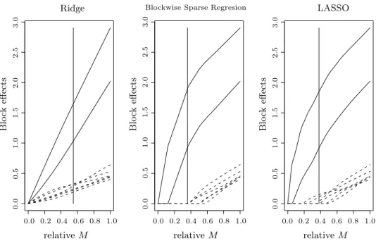
Figure 2.1 compares the ridge, LASSO and BSR methods on the simulated model whose details are given in Section 5.2. The simulated model has eight blocks, each of which consists of three covariates, and among which only the first two blocks are informative to responses and other six blocks are just noise. Figure 2.1 shows the paths of the norms of each block for various values of the restriction parameter M. The vertical line in the middle of the each plot represents the optimalM selected by 5-fold Cross Validation. It is clear that the BSR method outperforms the other two methods in terms of block selectivity. The correct two blocks are selected by the BSR while the LASSO includes some noise blocks. The Ridge is the worst since it includes all blocks.
378 YUWON KIM, JINSEOG KIM AND YONGDAI KIM PSfrag replacements 0.0 0.0 0.0 0.0 0.0 0.0 0.1 0.2 0.2 0.2 0.3 0.4 0.4 0.4 0.5 0.5 0.5 0.6 0.6 0.6 0.7 0.8 0.8 0.8 1.0 1.0 1.0 1.0 1.0 1.0 1.1 1.2 1.3 1.4 1.5 1.5 1.5 1.6 1.7 1.8 1.9 2.0 2.0 2.0 2.5 2.5 2.5 3.0 3.0 3.0 4.0
Blockwise Sparse Regresion Ridge Blo ck effects Blo ck effects Blo ck effects relative M relativeM relativeM LASSO 0 1 2 3 4 5 6 10,000 10 15 20 25 30 40 50 60 70
Figure 2.1. Paths of the norms of each block for example 1 in Section 5. The solid curves denote the signal blocks and the dashed curves denote the noise blocks. The vertical solid lines are positioned on the models selected by CV. The values in the horizontal axes are the ratios of the values of the restrictionM to the norms of the ordinary logistic regression solutions.
2.2. Algorithm
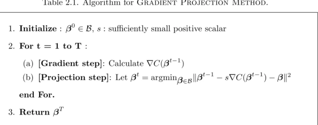
We first introduce the Gradient Projection Method, a well known technique for optimization on convex sets, and explain how to modify it for the BSR. Consider a constrained optimization problem given by
minimizing C(β) subject to β∈ B,
where B is a convex set. Let ∇C(β) be the gradient of C(β). The algorithm of the gradient projection method, which finds the solution by iterating between moving toward the opposite direction of the gradient and projecting it onto the constraint set B, is given in Table 2.1. If the gradient function is convex and Lipschitz continuous with the Lipschitz constant L, the sequence of solutions generated by the gradient projection method, with step sizes < 2/L, converges to the global optimum. s can be selected by calculating the Lipschitz constant
L or by trial and error. The speed of convergence does not depend strongly on the choice ofsunlesssis very small. For details of the algorithm, see Bertsekas (1999), and for its application to various constrained problems, see Kim (2004).
Table 2.1. Algorithm forGradient Projection Method.
1. Initialize: β0∈ B, s: sufficiently small positive scalar
2. For t = 1 to T :
(a) [Gradient step]: Calculate∇C(βt−1)
(b) [Projection step]: Letβt= argminβ∈Bkβt−1−s∇C(βt−1)−βk2
end For.
3. Return βT
For the BSR, we can easily check that the constraint set,B={Pp
j=1kβ(j)k ≤
M}, is convex, and so we can apply the gradient projection method. The hardest part of the algorithm is the projection (2b of Table 2.1. In general, computational cost here is large. However, for the BSR, projection can be done easily as follows. Let b = βt −s∇C(βt) and let b(j) be the jth block of b. Then βt+1 is the minimizer of p X j=1 kb(j)−β(j)k2 subject to p X j=1 kβ(j)k ≤M (2.1)
with respect to β. Suppose Mj =kβt+1(j)k are known for j = 1, . . . , p. Then, we
have
βt+1(j) =b(j) Mj
kb(j)k. (2.2)
So, for finding βt+1, it suffices to find Mjs. For Mj, plugging (2.2) to (2.1), we
solve the reduced problem as minimizing p X j=1 (kb(j)k −Mj)2 subject to p X j=1 Mj ≤M (2.3)
with respect toMjs withMj ≥0. For solving (2.3), note that if the projection of
(kb(1)k, . . . ,kb(p)k) onto the hyperplane of the form P
Mj =M has non-positive
values on some coordinates, then the solution of (2.3) should have exact zeros on those coordinates, which we call inactive. Once inactive coordinates are found, we rule out them and re-calculate the projection onto the reduced hyperplane until no more negative values occur in the projection. A small number, at most
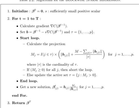
p, of iterations is required. Once we solve (2.3), we get βt+1 by (2.2). The procedure is summarized in Table 2.2.
380 YUWON KIM, JINSEOG KIM AND YONGDAI KIM
Table 2.2. Algorithm for theBlockwise Sparse Regression.
1. Initialize: β0=0, s: sufficiently small positive scalar
2. For t = 1 to T :
• Calculate gradient∇C(βt−1).
• Setb=βt−1−s∇C(βt−1) andτ ={1, . . . , p}.
• Start loop.
– Calculate the projection
Mj=I(j ∈τ)× kb(j)k+ M−P j∈τkb(j)k |τ| for j= 1, . . . , p.
where|τ|is the cardinality ofτ.
– If (Mj ≥0) for allj, then abort the loop. – Else update the active setτ ={j:Mj >0}.
• End loop.
• Get a new solution,βt(j)=b(j)
Mj
kb(j)k forj= 1, . . . , p.
end For.
3. Return βT
3. Selection of the restriction parameter M
In this section, we describe methods for selecting the restriction parameter
M of the BSR. One popular method for selectingM is the K-fold cross-validation (CV). However, the K-fold CV suffers from its computational burden. Another method is to use the generalized cross validation (GCV) proposed by Craven and Wahba (1979). A GCV type criterion for the LASSO is found in Tibshirani (1996), where the LASSO solution is approximated by the ridge solution. An extended GCV type criterion is proposed by Tibshirani (1997), where the LASSO technique is applied to the proportional hazard model.
We propose a GCV type criterion for the BSR, as in Tibshirani (1996, 1997). Suppose that all blocks have nonzero norms. When some blocks have zero norms, we reduce the design matrix by eliminating the blocks whose norms are zero. Using the relation, Pp
j=1kβ(j)k = Pp
j=1kβ(j)k2/kβ(j)k, ˆβ can be obtained as
the solution of minimizing
C(β) +λ 2 p X j=1 kβ(j)k2 kβ(j)k ,
for someλuniquely defined byM.Now, assuming that thekβˆ(j)kare known, we expect that the solution ˜β of minimizing
C(β) + λ 2 p X j=1 kβ(j)k2 kβˆ(j)k , (3.1)
gives an approximation to ˆβ. Let X denote the design matrix with x0
i as the
ith row and letη=Xβ. The iterative reweight least square method for solving (3.1) gives a linear approximation
˜
β≈(X0AX+λW)−1X0Az, (3.2)
where A = ∂2C(β)/∂ηη0, u = ∂C(β)/∂η, z = Xβ−A−1u and W is the
k×k diagonal matrix whose Pj−1 h=1dh+l
th diagonal element is 1/kβ(j)k for
j = 1, . . . , p, l = 1, . . . , dj, all evaluated at β = ˆβ. From (3.2), we construct a
GCV-type criterion GCV(M) = 1 n C( ˆβ) (1− p(M)n )2, where p(M) = tr[X(X0AX +λW)−1X0A] as in by Tibshirani (1997). We
agree that the GCV is a rough approximation, but we show that the GCV gives comparable performances to the 5-fold CV in the simulation study.
4. Standardization within Blocks
A common way of generating blocks is to use transformations such as polyno-mial or dummies from the original covariates. In many cases, there is more than one transformation. That results in the same model. Unfortunately, the block norm is not invariant with transformations. For example, consider a covariate x
having values on the three categories denoted by {1,2,3}. For dummy variables (z1, z2) to represent x,we can let (z1, z2) = (1,0) for x= 1, (z1, z2) = (0,1) for
x= 2,and (z1, z2) = (0,0) forx= 3.Suppose that the regression coefficients ofz1
andz2 are 1 and -1, respectively. In this case, the block norm becomes √2. Now,
we can use as dummy variables (z1, z2) = (1,0) for x = 1, (z1, z2) = (0,0) for
x = 2, and (z1, z2) = (0,1) for x = 3. The corresponding regression coefficients
become 2 and 1, and so the block norm is √5. Hence, different transformations may result in different block selections in the BSR. In this section, we propose a method of blockwise standardization of covariates to resolve this problem.
Let X1 and X2 be two design matrices of a given block such that there are
two regression coefficients β1 and β2 with X1β1 = X2β2. The blockwise
stan-dardization is based on the fact that kβ1k=kβ2k when X01X1 =X 0
382 YUWON KIM, JINSEOG KIM AND YONGDAI KIM
for some t > 0. Hence, when a design matrix for a block is given, we propose to orthogonalize the design matrix in advance, and then to estimate the corre-sponding regression coefficients using the BSR.
Specifically, let X be a design matrix partitioned intopsub-matrices (X(1),
. . . ,X(p)), whereX(j)corresponds to thejth block. For simplicity, we assume all columns ofX are centered at zero. Using the spectral decompositionX0
(j)X(j)=
P(j)Λ(j)P0
(j), where Λ(j) is the diagonal matrix with positive eigenvalues and
P(j) is the corresponding eigenmatrix, we can construct blockwise orthogonal design matrices as
Z(j)= √1
tj
X(j)T(j), (4.1)
for some tj >0 whereT(j)=P(j)Λ−1/2(j) . We can easily check Z0(j)Z(j) =t−j1I.
Fortj,we recommend using the number of positive eigenvalues ofX0(j)X(j).
This recommendation is motivated by the observation that the block norm tends to be larger when the size of the block is larger. Hence, blocks with more coef-ficients have more chance to be selected. With our recommendation, the deter-minants of Z0
(j)Z(j), j = 1, . . . , p, are all the same, and so the contribution of
each block to the response can be measured only by the norm of the regression coefficients.
To demonstrate the necessity of the recommended choice of tjs, we compare
the selectivity of the recommended choice of tjs with the choicetj = 1 for all j.
We generated 100 samples of 250 observations which consist of 14 independent uniform covariates (x1, . . . , x14) with range [−1,1] and responsey generated by a
logistic regression model with f(x) =x1. We assigned the covariates into three
blocks. Block 1 has the signal covariate x1, Block 2 has three noise covariates
(x2, x3, x4). The other ten noise covariates are assigned to Block 3. We
investi-gated which of Blocks 2 and 3 went to zero first as the restriction parameterM
decreased. When we usedtj = 1 for allj, Block 2 went to zero first in 96 samples
out of 100, which means that Block 3 was selected more frequently. When we used the recommended choice oftjs, Block 2 went to zero first in 58 samples out
of 100. That is, the recommended choice oftjs helped the ‘fair’ selection.
Once the solution β∗ with the blockwise standardized design matrix given
in (4.1) is obtained by the BSR, the coefficient β on the original design matrix is reconstructed asβ(j)=tj−1/2T(j)β∗(j).
5. Simulation 5.1. Outline
We compare the prediction error and the variable selectivity of the BSR with the ridge and LASSO on three examples with logistic regression models.
The restriction parameters of the three methods are chosen using GCV as well as 5-fold CV. Prediction errors are measured by the averages of test errors using two loss functions, the logistic loss (LOL) and the misclassification rate (MIR) on 10,000 randomly selected design points. The blockwise standardization is not used for the BSR to make the comparison fair.
5.2. Example 1
We generated 100 samples, each of which consisted of 250 observations. The covariates were generated from the 8-dimensional independent uniform distribu-tion on [−1,1]. The binary response y was generated by a logistic model with Pr(y = 1) = exp(f(x))/(1 + exp(f(x))) and Pr(y = 0) = 1−Pr(y = 1), where the true regression function is
f(x) = 2p1(x1) + 2p2(x1) + 2p3(x1) +p1(x2) +p2(x2) +p3(x2),
with p1(x) =x, p2(x) = (3x2−1)/2, andp3(x) = (5x3−3x)/2, the first three
Legendre polynomials. Thus all covariates except the first and second ones are pure noise.
The design matrix has 24 columns consisting of p1(xj), p2(xj) and p3(xj)
forj = 1, . . . ,8. The three columns of p1(xj), p2(xj) and p3(xj) from a original
covariate xj form a natural block. Consequently, we fit the logistic regression
model with the BSR penalty with the eight blocks, each of which has three regression coefficients. The ridge and LASSO penalty put restrictions on 24 individual regression coefficients.
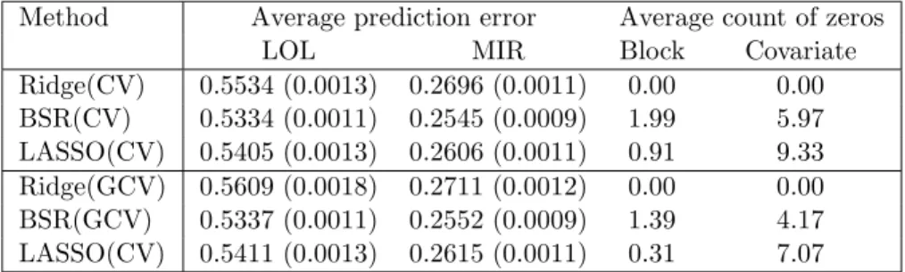
Table 5.3. The averaged prediction errors (standard errors) and averaged number of blocks and individual regression coefficients being zero from Ex-ample 1.
Method Average prediction error Average count of zeros
LOL MIR Block Covariate
Ridge(CV) 0.5534 (0.0013) 0.2696 (0.0011) 0.00 0.00 BSR(CV) 0.5334 (0.0011) 0.2545 (0.0009) 1.99 5.97 LASSO(CV) 0.5405 (0.0013) 0.2606 (0.0011) 0.91 9.33 Ridge(GCV) 0.5609 (0.0018) 0.2711 (0.0012) 0.00 0.00 BSR(GCV) 0.5337 (0.0011) 0.2552 (0.0009) 1.39 4.17 LASSO(CV) 0.5411 (0.0013) 0.2615 (0.0011) 0.31 7.07
The results are shown in Table 5.3. The BSR had the lowest prediction error, followed by LASSO. For variable selectivity, LASSO solutions included fewer variables but more blocks than did BSR solutions.
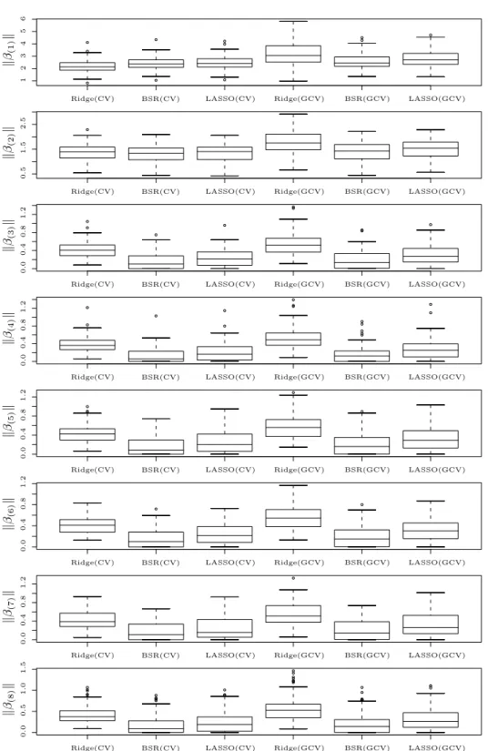
The box plots of the norm of each block are presented in Figure 5.2. It is clear that the norms of the noise blocks (blocks generated fromx3, . . . , x8) from
384 YUWON KIM, JINSEOG KIM AND YONGDAI KIM PSfrag replacements 0.0 0.0 0.0 0.0 0.0 0.0 0.1 0.2 0.3 0.4 0.4 0.4 0.4 0.4 0.5 0.5 0.6 0.7 0.8 0.8 0.8 0.8 0.8 1.0 1.1 1.2 1.2 1.2 1.2 1.2 1.3 1.4 1.5 1.5 1.6 1.7 1.8 1.9 2.0 2.5 3.0 4.0 Blockwise Sparse Regresion
Ridge Block effects relativeM LASSO 0 1 2 3 4 5 6 10,000 10 15 20 25 30 40 50 60 70 Ridge(CV) Ridge(CV) Ridge(CV) Ridge(CV) Ridge(CV) Ridge(CV) Ridge(CV) Ridge(CV) BSR(CV) BSR(CV) BSR(CV) BSR(CV) BSR(CV) BSR(CV) BSR(CV) BSR(CV) LASSO(CV) LASSO(CV) LASSO(CV) LASSO(CV) LASSO(CV) LASSO(CV) LASSO(CV) LASSO(CV) Ridge(GCV) Ridge(GCV) Ridge(GCV) Ridge(GCV) Ridge(GCV) Ridge(GCV) Ridge(GCV) Ridge(GCV) BSR(GCV) BSR(GCV) BSR(GCV) BSR(GCV) BSR(GCV) BSR(GCV) BSR(GCV) BSR(GCV) LASSO(GCV) LASSO(GCV) LASSO(GCV) LASSO(GCV) LASSO(GCV) LASSO(GCV) LASSO(GCV) LASSO(GCV) k β(1) k k β(2) k k β(3) k k β(4) k k β(5) k k β(6) k k β(7) k k β(8) k
5.3. Example 2
In this example, we only change the regression function in Example 1 to be more suitable to LASSO. The true regression function is
f(x) = 2p1(x1) + 2p2(x2) + 2p3(x3) +p1(x4) +p2(x5) +p3(x6),
where only one column amongp1(xj), p2(xj) andp3(xj) is related to the response
forj= 1, . . . ,6, andx7 and x8 are pure noises.
The results are shown in Table 5.4, where LASSO outperforms the others in prediction accuracy and the BSR is slightly better than the ridge. For variable selectivity, the BSR does not work well since it includes too many noise covariates. This is partly because the BSR includes all covariates in the block when the block has nonzero norm.
Table 5.4. The averaged prediction errors (standard errors) and averaged number of blocks and individual regression coefficients being zero from Ex-ample 2.
Method Average prediction error Average count of zeros
LOL MIR Block Covariate
Ridge(CV) 0.5148 (0.0012) 0.2523 (0.0009) 0.00 0.00 BSR(CV) 0.5117 (0.0013) 0.2499 (0.0010) 0.48 1.44 LASSO(CV) 0.5018 (0.0012) 0.2428 (0.0010) 0.48 10.05 Ridge(GCV) 0.5229 (0.0017) 0.2530 (0.0010) 0.00 0.00 BSR(GCV) 0.5156 (0.0015) 0.2506 (0.0010) 0.20 0.60 LASSO(CV) 0.5031 (0.0013) 0.2441 (0.0010) 0.09 7.14 5.4. Example 3
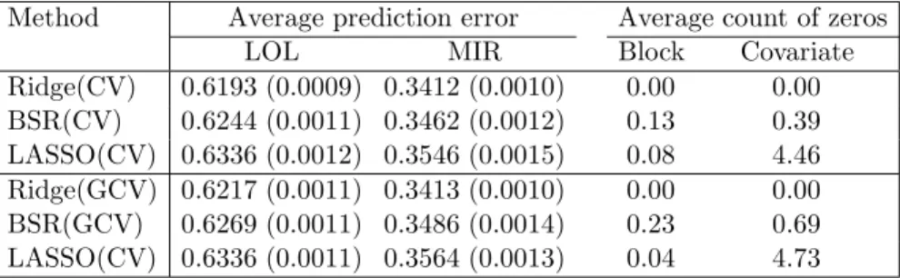
We try a different model from that in Example 1 to be more suitable to the ridge. Here f(x) = 8 X j=1 1 2(p1(xj) +p2(xj) +p3(xj)).
Table 5.5. The averaged prediction errors (standard errors) and averaged number of blocks and individual regression coefficients being zero from Ex-ample 3.
Method Average prediction error Average count of zeros
LOL MIR Block Covariate
Ridge(CV) 0.6193 (0.0009) 0.3412 (0.0010) 0.00 0.00 BSR(CV) 0.6244 (0.0011) 0.3462 (0.0012) 0.13 0.39 LASSO(CV) 0.6336 (0.0012) 0.3546 (0.0015) 0.08 4.46 Ridge(GCV) 0.6217 (0.0011) 0.3413 (0.0010) 0.00 0.00 BSR(GCV) 0.6269 (0.0011) 0.3486 (0.0014) 0.23 0.69 LASSO(CV) 0.6336 (0.0011) 0.3564 (0.0013) 0.04 4.73
386 YUWON KIM, JINSEOG KIM AND YONGDAI KIM
The results are shown in Table 5.5. For prediction accuracy, the ridge worked the best, the BSR next and LASSO the worst. Note that the BSR selects most of variables while LASSO fails to detect significant amount of covariates. That is, the BSR is better in variable selectivity than LASSO.
6. Examples
6.1. German credit data
German credit data consists of 1,000 credit histories with a binary response, and 20 covariates. The binary response represents good (700 cases) and bad cred-its (300 cases), respectively. Seven covariates are numerical and the rest are cate-gorical, with the number of categories ranging from 2 to 10. The data set is avail-able from UCI Machine Learning Repository (http://www.ics.uci.edu/∼mlearn/ MLRepository.html). The 20 covariates are given below.
V1 :Status of existing checking account (4 categories). V2 :Duration in month (numerical).
V3 :Credit history (5 categories). V4 :Purpose (10 categories). V5 :Credit amount (numerical).
V6 :Savings account/bonds (5 categories). V7 :Present employment since (5 categories).
V8 :Installment rate in percentage of disposable income(numerical). V9 :Personal status and sex (4 categories).
V10 :Other debtors / guarantors (3 categories). V11 :Present residence since (numerical). V12 :Property (4 categories).
V13 :Age in years (numerical).
V14 :Other installment plans (3 categories). V15 :Housing (3 categories).
V16 :Number of existing credits at this bank (numerical). V17 :Job (4 categories).
V18 :Number of people being liable to provide maintenance for (numerical). V19 :Telephone (2 categories).
V20 :Foreign worker (2 categories).
We expand each of the numerical covariates to a block using transformations up to the 3th order polynomial, and each of the categorical covariates to a block with the corresponding dummy variables. The blocks are standardized as in (4.1). Then, the logistic regression model with blockwise restriction is fitted, where the restriction parameter M is chosen by GCV. For GCV, we used the 0-1 loss in the numerator instead of the log-likelihood, for the former tends to yield better models.
BLOCKWISE SPARSE REGRESSION 387
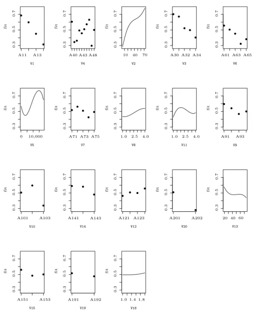
The BSR eliminates the covariatesV16andV17, whose block norms are zero.
The partial fits on the remaining 18 covariates are shown in Figure 6.3, where the covariates with larger block norms appear first. This suggests that V1 and V4are the most important covariates.
0.1 0.2 0.3 0.3 0.3 0.3 0.3 0.3 0.3 0.3 0.3 0.3 0.3 0.3 0.3 0.3 0.3 0.3 0.3 0.3 0.4 0.5 0.5 0.5 0.5 0.5 0.5 0.5 0.5 0.5 0.5 0.5 0.5 0.5 0.5 0.5 0.5 0.5 0.5 0.6 0.7 0.7 0.7 0.7 0.7 0.7 0.7 0.7 0.7 0.7 0.7 0.7 0.7 0.7 0.7 0.7 0.7 0.7 0.8 1.0 1.0 1.0 1.1 1.2 1.3 1.4 1.5 1.6 1.7 1.8 1.9 2.0 2.5 2.5 3.0 4.0 4.0
Blockwise Sparse Regresion
Ridge Block effects relativeM LASSO 0 1 2 3 4 5 6 10,000 10 15 20 25 30 40 40 50 60 70 Ridge(CV) BSR(CV) LASSO(CV) Ridge(GCV) BSR(GCV) LASSO(GCV) kβ(1)k kβ(2)k kβ(3)k kβ(4)k kβ(5)k kβ(6)k kβ(7)k kβ(8)k V1 V4 V2 V3 V5 V6 V7 V8 V9 V10 V11 V12 V13 V14 V15 V16 V17 V18 V19 V20 fit fit fit fit fit fit fit fit fit fit fit fit fit fit fit fit fit fit
A11 A13 A40 A43 A48 A30 A32 A34 A61 A63 A65
A71 A73 A75 A91 A93
A101 A103 A141 A143 A121 A123 A201 A202
A151 A153 A191 A192
Figure 6.3. The partial fits on 18 selected covariates in German credit data.
We compare the prediction accuracies of the BSR with those of the ridge and LASSO. The misclassification rates are estimated by 10 repetitions of the
388 YUWON KIM, JINSEOG KIM AND YONGDAI KIM
10-fold CV. For each repetition, the restriction parameters are chosen by GCV. The results summarized in Table 6.6 show that the LOL and MIS of the BSR and LASSO are close, and that the ridge does less well.
Table 6.6. Estimates of LOL and MIS and their standard errors in German credit data.
Method LOL MIS
Ridge 0.6926 (0.0008) 0.2446 (0.0014) BSR 0.6882 (0.0011) 0.2399 (0.0020) LASSO 0.6888 (0.0010) 0.2399 (0.0020)
6.2. Breast cancer data
The second example is the Breast cancer data, available from UCI Machine Learning Repository (http://www.ics.uci.edu/∼mlearn/MLRepository.html). The data set includes nine covariates and a binary response. The response has “no-recurrence-events” in 201 cases, which are coded to 0, and “recurrence-events” in 85 cases, which are coded to 1. Five covariates are categorical and four covariates are numerical.
We expand covariates as was done for the German credit data. The BSR eliminates three covariates and the partial fits on remaining six covariates are shown in Figure 6.4. PSfrag replacements 0.0 0.1 0.2 0.3 0.4 0.4 0.4 0.4 0.4 0.4 0.5 0.5 0.5 0.5 0.5 0.5 0.6 0.6 0.6 0.6 0.6 0.6 0.7 0.7 0.7 0.7 0.7 0.7 0.8 1.0 1.1 1.2 1.3 1.4 1.5 1.6 1.7 1.8 1.9 2.0 2.5 3.0 4.0
Blockwise Sparse Regresion Ridge Block effects relativeM LASSO 0 1 2 3 4 5 6 10,000 10 10 15 20 25 20 30 40 50 60 70 Ridge(CV) BSR(CV) LASSO(CV) Ridge(GCV) BSR(GCV) LASSO(GCV) kβ(1)k kβ(2)k kβ(3)k kβ(4)k kβ(5)k kβ(6)k kβ(7)k kβ(8)k V1 V2 V3 V4 V5 V6 V7 V8 V9 V10 V11 V12 V13 V14 V15 V16 V17 V18 V19 V20 fit fit fit fit fit fit A11 A13 A40 A43 A48 A30 A32 A34 A61 A63 A65 A71 A73 A75 A91 A93 A101 A103 A141 A143 A121 A123 A201 A202 A151 A153 A191 A192 no no yes yes deg-malig irradiat node-caps menopause inv-nodes tumor-size ge40 lt40 premeno
Figure 6.4. The partial fits on 6 selected covariates in Breast Cancer data.
repetitions of the 10 fold CV are summarized in Table 6.7, which shows that the BSR is the best in prediction accuracy.
Table 6.7. Estimates of LOL and MIS and their standard errors in Breast cancer data.
Method LOL MIS
Ridge 0.6976 (0.0028) 0.2700 (0.0052) BSR 0.6917 (0.0015) 0.2578 (0.0028) LASSO 0.6964 (0.0016) 0.2646 (0.0028)
7. Concluding Remarks
Even though we focused on logistic regression the proposed method can be applied to many problems, such as Poisson regression and the proportional hazard model. The only modification required for such extensions is to calculate the corresponding gradient.
There are various possible extensions of the BSR. For example, we can com-bine the idea of blockwise sparsity with other sparse penalties such as SCAD, fused LASSO or the elastic net mentioned in the Introduction. We believe that the computational algorithm proposed in this paper is general enough to be easily modified for such extensions.
The asymptotic properties of the BSR can be derived following Knight and Fu (2000). This is important for variance estimation of the estimated regression coefficients. We will pursue this problem in the near future.
Acknowledgement
This research was supported (in part) by the SRC/ERC program of MOST/ KOSEF (R11-2000-073-00000).
References
Bakin, S. (1999). Adaptive regression and model selection in data mining problem. Ph.D. thesis, Australian National University, Australia.
Bertsekas, D. P. (1999). Nonlinear Proramming. Athena Scientific, Belmount, Massachusettes. Second edition.
Chen, S. S., Donoho, D. L. and Saunders, M. A. (1999). Atomic decomposition by basis pursuit.
SIAM J. Sci. Comput. 20, 33-61.
Craven, P. and Wahba, G. (1979). Smoothing noisy data with spline functions. J. Amer. Statist. Assoc. 31, 377-403.
Fan, J. and Li, R. (2001). Variable selection via noncocave penalized likelihood and its oracle properties. J. Amer. Statist. Assoc. 96, 1348-1360.
Gunn, S. R. and Kandola, J. S. (2002). Structural modelling with sparse kernels. Machine Learning 48, 137-163.
390 YUWON KIM, JINSEOG KIM AND YONGDAI KIM
Kim, Y. (2004). Gradient projection method for constrained estimation, unpublished man-uscript. (available at http://stats.snu.ac.kr/∼gary).
Knight, K. and Fu, W. J. (2000). Asymptotics for lasso-type estimators. Ann. Statist. 28, 1356-1378.
Krishnapuram, B., Carlin, L., Figueiredo, M. A. T. and Hartemink, A. (2004). Learning sparse classifier: Multi-class formulation, fast algorithms and generalization bounds. Technical report, ISDS, Duke university.
Lin, Y. and Zhang, H. (2003). Component Selection and Smoothing in Smoothing Spline Analysis of Variance Models. Technical Report 1072, Department of Statistics, University of Wisconsin-Madison.
Roth, V. (2004). The generalized lasso. IEEE Trans. Neural Networks15, 16-28.
Tibshirani, R. (1996). Regression shirinkage and selection via the lasso. J. Roy. Statist. Soc. Ser. B58, 267-288.
Tibshirani, R. (1997). The Lasso method for variable selection in the Cox model. Statist. medicine16, 385-395.
Tibshirani, R., Rosset, S., Zhu, J. and Knight, K. (2005). Sparsity and smoothness via the fused lasso. J. Roy. Statist. Soc. Ser. B67, 91-108.
Zhang, H., Wahba, G., Lin, Y., Voelker, M., Ferris, M., Klein, R. and Klein, B. (2003). Vari-able selection and model building via likelihood basis pursuit. Technical Report 1059r, Department of Statistics, University of Wisconsin, Madison, WI.
Yuan, M. and Lin, Y. (2004). Model selection and estimation in regression with grouped vari-ables. Technical Report 1095, Department of Statistics, University of Wisconsin, Madison, WI.
Zou, H. and Hastie, T. J. (2004). Regularization and variable selection via elastic net. Technical report, Department of Statistics, Stanford University.
Statistical Research Center for Complex Systems, Seoul National University, Korea. E-mail: [email protected]
Statistical Research Center for Complex Systems, Seoul National University, Korea. E-mail: [email protected]
Department of Statistics, Seoul National University, Korea E-mail: [email protected]