Workload Models and Performance Evaluation of Cloud Storage Services

.

Workload Models and Performance

Evaluation of Cloud Storage Services

RT.DCC.003/2015

Glauber D. Gonçalves

Idilio Drago

Alex Borges Vieira

Ana Paula Couto da Silva

Jussara Marques de Almeida

Marco Mellia

OUTUBRO

2015

UFMG

-

ICE

DEPARTAMENTO

DE

CIÊNCIA

DA

C

O

M

P

U

T

A

Ç

Ã

O

Workload Models and Performance Evaluation of

Cloud Storage Services

Glauber D. Gon¸calvesa,∗_{, Idilio Drago}b_{, Alex B. Vieira}c_{, Ana Paula Couto da}

Silvaa_{, Jussara M. Almeida}a_{, Marco Mellia}b

a

Universidade Federal de Minas Gerais, Brazil

b

Politecnico di Torino, Italy

c

Universidade Federal de Juiz de Fora, Brazil

Abstract

Cloud storage systems are currently very popular with many companies offering services, including worldwide providers such as Dropbox, Microsoft and Google. These companies as well as providers entering the market could greatly benefit from a deep understanding of typical workload patterns their services have to face in order to develop cost-effective solutions. Yet, despite recent studies of usage and performance of these systems, the underlying processes that generate workload to the system have not been deeply studied.

This paper presents a thorough investigation of the workload generated by Dropbox customers. We propose a hierarchical model that captures user ses-sions, file system modifications and content sharing patterns. We parameter-ize our model using passive measurements gathered from 4 different networks. Next, we use the proposed model to drive the development of CloudGen, a new synthetic workload generator that allows the simulation of the network traf-fic created by cloud storage services in various realistic scenarios. We validate CloudGen by comparing synthetic traces with actual data from operational networks. We then show its applicability by investigating the impact of the continuing growth in cloud storage popularity on bandwidth consumption. Our results indicate that a hypothetical 4-fold increase in both user population and content sharing could lead to 30 times more network traffic. CloudGen is a valuable tool for administrators and developers interested in engineering and deploying cloud storage services.

Keywords: Cloud Storage, Models, Measurements

∗_{Corresponding author}

Email addresses: [email protected](Glauber D. Gon¸calves),

[email protected](Idilio Drago),[email protected](Alex B. Vieira), [email protected];(Ana Paula Couto da Silva),[email protected](Jussara M. Almeida),[email protected](Marco Mellia)

1. Introduction

Cloud storage is a data-intensive Internet service that synchronizes files with the cloud and among different end user devices, such as PCs, tablets and smart-phones. It offers the means for customers to easily backup data and to perform collaborative work, with files being automatically uploaded and synchronized. Cloud storage is already one of the most popular Internet services, generating a significant amount of traffic [1]. Well-established players such as Dropbox, as well as giants like Google and Microsoft, face a fierce competition for customers.

Currently, Dropbox leads the market with more than 400 million users by 2015,1

and Google and Microsoft show a fast growth [2], thanks to solutions that are more and more integrated into Windows or Android Operating Systems.

Both established and new players could greatly benefit from a deep under-standing of the workload patterns that cloud storage services have to face in order to develop cost-effective solutions. However, several aspects make the analysis of cloud storage workloads a challenge. As the stored content is private and synchronization protocols are mostly proprietary, the knowledge of how these systems work is limited outside companies running the services. It is thus very hard to obtain large scale data that could drive workload analyses, given also the widespread use of encryption for both data and control messages [3].

Indeed, we are aware of only a few recent efforts to analyze the characteristics of cloud storage services [1], focusing either on architectural design aspects [4, 5], quality of experience [6, 7], or benchmark-driven performance studies [3, 8, 9]. Yet, a characterization of the underlying client processes that generate workload to the system, notably the data transfer patterns that emerge from such pro-cesses, is only partly addressed by our preliminary efforts presented in [10, 11]. Such knowledge is key to analyze the impact of these services on network band-width requirements as well as to the design of future services.

Towards filling this gap, this paper performs a thorough investigation of the workload experienced by Dropbox, the currently most popular cloud storage service. We propose a hierarchical model that describes client behavior in suc-cessive Dropbox sessions. Within each session, our model captures file system modifications and content sharing among users and devices, as well as client interactions with Dropbox servers while storing and retrieving files. We param-eterize the model based on the analysis of Dropbox traffic traces collected in four different networks, namely two university networks – one in South America and one in Europe, and two European Internet Service Provider (ISP) networks. We offer these traces to the community, to foster future studies.

Next, we use the model to drive the development of a new synthetic

work-load generator, called CloudGen. Our validation experiments, comparing real

and synthetic workloads, show that CloudGen is able to reproduce the behavior of Dropbox customers. CloudGen is a valuable tool that allows network ad-ministrators and cloud storage developers to analyze the traffic volume of cloud

storage as well as to evaluate future system optimization and developments in various synthetic, but still realistic, workload scenarios.

Given the steady increase in Dropbox user base [12], we illustrate the appli-cability of CloudGen by evaluating how network traffic would change in edge networks, such as ISP and campus networks, when customer population grows and when users share more content via cloud storage. Our results suggest that a hypothetical 4-fold increase in both user population and content sharing could lead to 30 times more cloud storage traffic, eventually challenging the capacity of such systems.

In sum, our main contributions are the following:

• We propose a hierarchical model of the Dropbox client behavior and

pa-rameterize it using passive measurements gathered from 4 different net-works. To the best of our knowledge, we are the first to model the client behavior and data sharing in Dropbox.

• We develop and validate a synthetic workload generator (CloudGen) that

reproduces user sessions, traffic volume and data sharing patterns. We

offer CloudGen as free software to the community.2

• We illustrate the applicability of CloudGen in a case study, where the

impact of larger user populations and more content sharing are explored. This paper extends our previous efforts to model Dropbox client behav-ior [10, 11]. Specifically, unlike in [10], our new model explicitly captures data sharing and modifications. We also build on top of the proposed model by developing and validating a new workload generator, which was introduced in our preliminary work in [11], and we use the workload generator to analyze the network traffic of cloud storage services in hypothetical future scenarios.

The paper is organized as follows. Section 2 presents the background on Dropbox. Our data collection methodology is presented in Section 3. Section 4 describes our client behavior model and characterizes its components, whereas our workload generator is introduced in Section 5. We illustrate CloudGen applicability in Section 6, exploring possible future scenarios for cloud storage usage. Section 7 reviews related work, while Section 8 summarizes our contri-butions and lists future work. Finally, additional details of the characterization of our model components are provided in Appendix A.

2. Overview of Dropbox

2.1. Architecture

Dropbox relies on thousands of servers that are split into two major groups: control andstorageservers. Control servers are responsible for: (i) user authen-tication; (ii) management of the Dropbox file system metadata; and (iii)

agement of device sessions. Storage servers are in charge of the actual storage of data, and are outsourced to the Amazon cloud by the time of writing.

Users can link several devices to Dropbox using both PC and mobile clients. Web interfaces are also available, providing an easy way to access files in the cloud. We focus only on PC clients in this work, since they are responsible for most workload in cloud storage [1], although our model and workload generator can be trivially extended to other usage scenarios as well.

Every user registered with Dropbox is assigned a uniqueuser ID. Every time

Dropbox is installed on a PC, it provides the PC a uniquedevice ID. Users need

to select an initial folder in their PCs from where files are kept synchronized with the remote Dropbox servers. Users might decide to share content with other users. This is achieved by selecting a particular folder that is shown to

every participant in the sharing as ashared folder.

Internally, Dropbox treats the initial folders selected at configuration time

and all shared folders indistinctly. They are all called namespaces, and each

is identified by a uniquenamespace ID. Namespaces are usually synchronized

with all devices of the user and, for shared folders, with all devices of all users participating in the sharing. Each namespace is also attached to a monotonic journal ID (JID), representing the namespace latest version [13].

We refer the reader to [1] for details of the architecture of Dropbox. 2.2. Client Protocols

Our work takes as reference the protocols used by Dropbox in its client

v2.8.4.3 _{A device connecting to Dropbox contacts control servers to perform}

user authentication and to send its list of namespaces and respective journal IDs. This step allows servers to decide whether the device is updated or if it needs to be synchronized. If outdated, the device executes storage operations (exemplified next), until it becomes synchronized with the cloud. After that, the device finishes the initial synchronization phase and enters in steady state. When a Dropbox device identifies new local changes (e.g., new files, or file modifications), it starts a synchronization cycle. The device first performs sev-eral local operations to prepare files for synchronization. For example, Dropbox splits files in chunks of up to 4 MB and calculates content hashes for each of them. Chunks are compressed locally, and they might be grouped into bundles to improve performance [3].

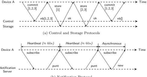
As soon as chunks/bundles are ready for transmission, the device behaves as depicted in Figure 1a. It first contacts a Dropbox control node, sending a list of

new chunk hashes – see thecommit request in the left-hand side of Figure 1a.

The servers answer with the subset of hashes that is not yet uploaded (seeneed

blocks (nb)reply). Note that servers can skip requesting chunks it already has, a mechanism known as client-side deduplication [14]. If any hash is unknown to servers, the device executes several storage operations directly with the storage

3_{Note that our model is applicable to other cloud storage systems and Dropbox versions}

Control Storage Device A Time commit [1,2,3] nb[1,2,3] store [1] ok store [2,3] ok commit [1,2,3] nb[]

(a) Control and Storage Protocols

Notification Server

Device A Time

subscribe subscribe subscribe

punt punt new

Heartbeat (_≈60s) Heartbeat (_≈60s) Asynchronous

(b) Notification Protocol

Figure 1: Basic operation of Dropbox client protocols.

servers (see store requests).4 _{Finally, the device contacts again the Dropbox}

control node, repeating the initial procedure to complete the transaction. Since the login and until going off-line, devices keep open a connection with

a Dropbox control server, which we callnotification server. Notification servers

are in charge of spreading information about changes performed in namespaces. For instance, when a partner in a shared folder performs changes, notifications are sent to all devices participating in the sharing. Devices then contact the Dropbox storage and control centers to retrieve updates.

The notification protocol is illustrated in Figure 1b. As soon as a device

connects to Dropbox, it contacts a notification server (see subscribe request).

Contrary to other Dropbox communications that have always been performed over SSL/TLS, the traffic to notification servers used to be exchanged in plain text HTTP during the period our datasets were collected. Every message sent to notification servers contains a device ID and a user ID, as well as the full list of namespaces in the client with their repetitive journal IDs.

Notification servers answer after approximately 60 s if no changes in

names-paces are performed in the meanwhile (seepuntreply). The arrival of an answer

triggers the client to resend asubscriberequest, thus acting like a heartbeat

pro-tocol. If any changes are detected in a namespace, the servers instead answer

to the pending request asynchronously, with a new message. The client then

reacts to the notification, starting a new synchronization as in Figure 1a.

4_{Dropbox also deploys a protocol for synchronizing devices in Local Area Networks, called}

LAN Sync. Devices in a LAN can use it to exchange files without retrieving content from the cloud. Since such traffic does not travel outside the LAN, we ignore the effects of LAN Sync.

Table 1: Overview of our datasets.

Name Devices Upload

(TB) Download (TB) Namespaces Changes 1 _Period Campus-1 12,587 1.7 3.8 10,609 2,690,617 04/14–06/14 Campus-2 1,987 0.6 1.0 9,861 507,394 04/14–06/14 PoP-1 9,478 3.9 6.8 28,899 1,657,744 10/13–04/14 PoP-2 3,376 2.4 3.7 12,050 1,306,045 07/13–05/14 Total 27,428 8.6 15.3 61,418 6,161,800 –

1_{Number of times the journal ID of a namespace has changed.}

By observing traffic to notification servers, it is possible to identify when each namespace is changed. We explore these messages to trace the evolution of namespaces of Dropbox clients and reconstruct client behavior.

3. Datasets and Methodology

3.1. Datasets

We rely on Tstat [15] to perform passive measurements and collect data related to Dropbox from different networks. Tstat monitors each TCP con-nection, exposing flow level information, including: (i) anonymized client IP addresses; (ii) timestamps of the first and the last packets with payload in each flow; (iii) the amount of exchanged data; and (iv) the Fully Qualified Domain Name (FQDN) the client resolved via DNS queries prior to open the flow [16].

We adopt a methodology similar to the one in [1] to filter and classify Drop-box traffic. Specifically, we take advantage of the FQDNs exported by Tstat to filter records related to the several Dropbox servers. For example, we iso-late flow records reiso-lated to the storage of data by looking for FQDNs contain-ingdl-client*.dropbox.com. Similarly, we usenotify*.dropbox.com to filter flow records associated with the notification of changes and heartbeat messages.

In addition to TCP level flows, we use the HTTP monitoring plug-in of Tstat to export, simultaneously to the flows, information seen in heartbeat messages (see Section 2.2). For each event, we gather: (i) the timestamp of the event; (ii) the device ID related to the event; (iii) the user ID related to the event; (iv) each namespace ID registered in the device; and (v) the latest journal ID

of each namespace.5

We have collected traffic in 4 different networks, including University cam-puses and ISP networks. Table 1 summarizes our datasets, presenting the num-ber of Dropbox devices, the Dropbox traffic volume, the numnum-ber of unique namespaces, the number of times the journal ID of a namespace has changed, and the data capture period.

5_{Our data does not include any information that could reveal user identities, or information}

about the content users store in Dropbox. IP addresses are anonymized directly in the probes, whereas all Dropbox IDs are numeric keys that offer no hints about users’ identities.

Campus-1 and Campus-2 datasets have been collected at border routers of two distinct campus networks. Campus-1 includes traffic of a large South American university with user population (including faculty, student and staff)

of≈57,000 people. Campus-2 serves around≈15,000 users in a European

uni-versity. Both datasets include traffic generated by wired workstations in research and administrative offices, whereas Campus-1 includes also WiFi networks.

PoP-1 and PoP-2 have been collected at distinct Points of Presence (PoPs)

of a European ISP, aggregating more than 25,000 and 5,000 households,

re-spectively. ADSL lines provide access to 80% of the users in PoP-1, while Fiber To The Home (FTTH) is available to the remaining 20% of users in PoP-1 and to all users in PoP-2. Ethernet and/or WiFi are used at home to connect end users’ devices, such as PCs or smartphones.

In total, we have observed more than 20 TB of data exchanges with Drop-box servers, 27 k unique DropDrop-box devices and 61 k unique namespaces during approximately 1 year of data collections. Our datasets provide not only a large-scale view in terms of number of users/devices, but also a rich and longitudinal picture of the Dropbox usage. A key contribution of our work is the release of anonymized data to the public, aiming to foster new researches and independent validations of our work. We invite interested readers to contact us in order to access the datasets.

3.2. Data Preparation

Our data capture resulted in two distinct and independent types of datasets for each analyzed network: (i) flow information that includes the data volume exchanged by clients with Dropbox storage servers; (ii) heartbeat messages with metadata related to the Dropbox namespaces. However, these two data sources have no common keys to provide an association between notifications of changes in namespaces and storage flows (i.e., data volume). Even more, we observe no one-to-one correspondence between notifications and flows. Indeed, files of different transactions might be exchanged in a single TCP flow, whereas a single transaction might be split across several TCP flows [3].

Our goal is to model and characterize the behavior of devices connected to Dropbox. As we will show later, our model requires knowledge about (i) how frequently namespaces are changed, and (ii) how much data is uploaded and/or downloaded to/from Dropbox servers. To extract this information, we develop a method to estimate the uploaded/downloaded volume that corresponds to each notification of changes in namespaces. The method works in three steps.

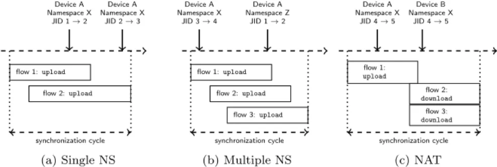
First, we group all flows and heartbeat messages per client IP address. How-ever, IP addresses provide only a coarse identification of devices in Dropbox ses-sions, since different devices may be present behind NAT – e.g., when sharing the same Internet access line at home. We leverage the heartbeat messages to identify precisely when each device becomes active and inactive, even if several devices are simultaneously connected from a single IP address.

Second, we group all flows overlapping in time for each anonymized IP ad-dress. We define the total overlapping period as a synchronization cycle. Thus,

flow 1:upload flow 2:upload synchronization cycle Device A Namespace X JID 1→2 Device A Namespace X JID 2→3 (a) Single NS flow 1:upload flow 2:upload flow 3:upload synchronization cycle Device A Namespace X JID 3→4 Device A Namespace Z JID 1→2 (b) Multiple NS flow 1: upload flow 2: download flow 3: download synchronization cycle Device A Namespace X JID 4→5 Device B Namespace X JID 4→5 (c) NAT

Figure 2: Examples of the most common cases processed by our method to label notifications and to estimate the transferred volumes (NS stands for namespace).

during a synchronization cycle, at least one device is uploading and/or down-loading content. Considering the Dropbox protocols, notifications of changes must appear during synchronization cycles or shortly before/after their be-gin/end. We thus form a list of notifications – from the same anonymized IP address – announced during each synchronization cycle, considering a small threshold (60 s, in-line with the heartbeat interval) for merging notifications before/after the synchronization cycle.

Third, we evaluate each synchronization cycle to decide whether notifications represent uploads or downloads, and then to assign volumes to the notifications. We first label each data flow in the synchronization cycle as upload or download. We are able to do so because Dropbox typically performs either uploads or downloads in a single TCP flow, opening parallel flows when both operations need to be performed simultaneously [3]. Therefore, we label flows simply by inspecting their downstream and upstream volumes. Then, we inspect metadata in notifications (e.g., device and namespace IDs) to decide how to distribute upload and download volumes among notifications.

Figure 2 provides the most common cases we notice while assigning volumes to notifications. Figure 2a presents a scenario where a Device A performs several uploads to a single namespace. In this case we label all notifications as upload. Moreover, the total synchronization cycle volume is equally divided among the notifications. We apply the same methodology for symmetric cases, in which a unique device performs several downloads from a single namespace.

Often, a device updates multiple namespaces simultaneously. This case is illustrated in Figure 2b, in which Device A updates Namespaces X and Z during the same synchronization cycle. It occurs typically after a device connects to the Internet: If modifications in several namespaces are performed while the device is off-line, all namespaces must be synchronized at once. We are able to label all notifications as upload, but we cannot match single flows to notifications. Thus, for simplicity, we equally divide the total volume among notifications. Again, we apply the same methodology in symmetric cases with only downloads.

Finally, Figure 2c presents a NAT scenario, e.g., when Dropbox is used to synchronize various devices in the same house with a single IP address. Note that we observe upload and download flows from the same address, and noti-fications for different devices, but always for a single namespace. We infer the label of notifications based on timestamps: Clearly, the first notification comes from the device uploading content, while remaining notifications come from de-vices downloading content. Thus, we assign the total upload volume to the first notification, and divide the total download volume equally among other devices. Some corner cases prevent us from estimating volume for notifications. We ignore flows and notifications in complex NAT scenarios, where multiple devices modify multiple namespaces simultaneously. We also ignore a small number of orphan notifications and orphan flows – i.e., we see notifications, but no simul-taneous storage flows, or vice-verse. Orphan notifications happen because the Dropbox client may generate no workload to storage servers when users perform

local modifications, such as when files are deleted or renamed or when theLAN

Sync actuates. Orphan flows and orphan notifications are also an outcome of

artifacts in our data capture: Packet loss during the capture might cause heart-beat messages to be missed. Finally, since we characterize namespace changes

by observing Journal IDtransitions, we ignore data flows that happen during

the first time a device is seen in our captures.

Despite these artifacts, our method is able to associate most volume to no-tifications. We associate 77% (60%) of the total volume of upload (download) with notifications in Campus-1, and 54% (44%) in Campus-2. Concerning PoP datasets, we associate 67% (57%) of the total volume of upload (download) in PoP-1, whereas that percentages are 77% (68%) in PoP-2. Percentages for downloads are consistently lower than for uploads thanks to new devices reg-istered with Dropbox during our captures – those typically download lots of contents during the initial synchronization cycle and we ignore this volume. Differences in percentages across datasets are in-line with the presence of NATs in each network and the packet loss rate in the respective probes.

4. Modeling the Dropbox Client

4.1. Assumptions

We target two aspects to build a model that captures the complexity of the Dropbox client functioning in a realistic fashion. First, our model needs to represent users’ behavior, including mechanisms to describe the arrival and departure of devices, as well as the dynamics behind modifications of Dropbox namespaces by the users. Second, from the users’ behavior, the model needs to estimate the resulting workload seen in the network.

We make some assumptions to simplify the model. First, we assume Dropbox

devices generate new content (i.e., modifications in namespace)independentlyof

any other device. That is, we assume the appearance of new contents that need to be uploaded to Dropbox servers is a process that can be modeled per device, without considering other devices from the same or other Dropbox users.

Session Layer

Namespace Layer

Data Transmission Layer

Login Logout Session Duration Login Inter-Session Time ... NS1 NS2 NS3 . . . N a m es p a ces p er D ev ice . . . Inter-Modification Times

Number of Modifications Number of Modifications

download -upload -upload -upload download

Figure 3: Model of the Dropbox client behavior.

Second, we assume that the upload of content to servers and its propagation to several devices follow the Dropbox protocols in Section 2. This implies our model follows two major design principles: (i) a device producing new content uploads it to the cloud immediately; (ii) all devices registering a namespace download updates performed elsewhere as soon as this is available at the cloud. Third, we assume content uploaded to a namespace is always propagated to all other devices registering the namespace. In practice, users’ actions might prevent a content from reaching other devices. For instance, users could man-ually pause content propagation in specific shared folders. More important, devices that stay off-line for long periods might return on-line after previously uploaded files are removed from Dropbox. We simplify our model by avoiding describing the evolution of namespaces in a per-file granularity. The model thus provides an upper bound for downloads caused by content propagation.

Finally, in this work we refrain from modeling the physical network or servers. We assume that data transmission or server delays are negligible. Mod-eling network conditions is out of our scope, and could be achieved by coupling our model to well-known network simulation approaches, such as in [17]. 4.2. Proposed Hierarchical Model

We propose a model composed by two parts: (i) the working dynamics of each Dropbox device in isolation; and (ii) the set of namespaces that is used to propagate content among devices.

4.2.1. Modeling Device Behavior

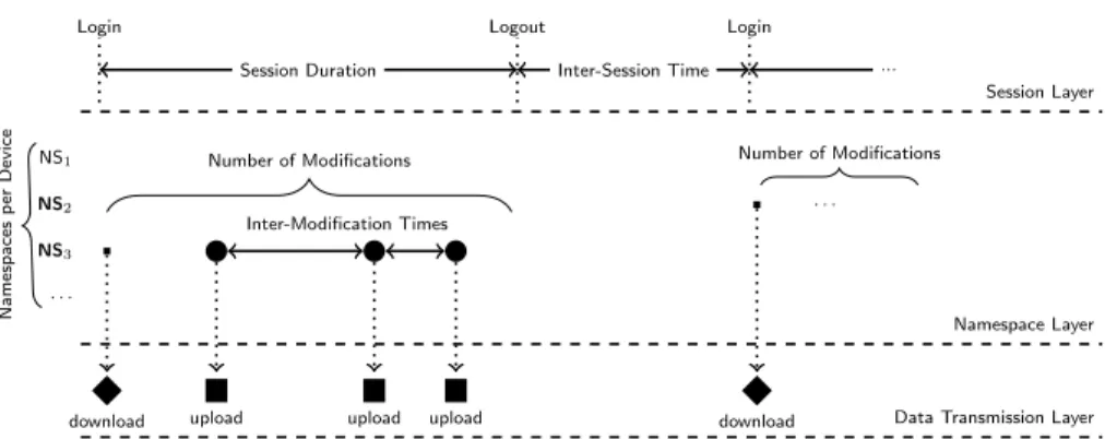
Figure 3 depicts how our model represents the working of a single Dropbox device. It captures three fundamental aspects to cloud storage clients: (i) the sessions of devices – i.e., devices becoming on-line and off-line; (ii) the frequency people make modifications in the file system that result in storage workload; (iii) the transmission of data from/to the cloud. Each aspect is encoded in a layer forming a hierarchical model for the Dropbox client behavior.

Thesession layer is the highest one in the hierarchy, describing the activity of devices. Thus, it is the one closest to the behavior of end users. While devices

are active, they might generate workload to storage servers, which is encoded in lower layers of the model. Yet, active devices generate workload to control servers, e.g., to notify changes in namespaces. A session starts when the device logs in, and it lasts until the device logs out. We call the duration of this interval thesession duration. The time between the client logout and its next login we

refer to as theinter-session time. Since we focus on PC clients, which usually

connect automatically in background, the inter-session time typically happens when devices are disconnected from the Internet.

The namespace layer encodes the modifications happening in namespaces.

Each device registers a number of namespaces, characterized by thenamespaces

per device component. Devices then may start several synchronization cycles. Synchronization cycles start because new content is produced locally and needs to be uploaded to the cloud, or because new content is produced elsewhere and needs to be downloaded by the device.

The start of uploads is regulated by three components: Thenamespace

se-lection, the number of modifications and the inter-modification time. The first determines which namespaces of the device have modifications that result in uploads during the session. The second represents the total number of uploads during the session. The third models the interval between consecutive uploads. Downloads are governed by the behavior of peer devices in the content propa-gation network, which we will describe next.

Finally, at thedata transmission layer, we characterize the size of the

work-loads locally produced at the device, which are sent to servers. The upload

volume is the single component in this layer. 4.2.2. Modeling the Content Propagation Network

Modifications in namespaces (i.e., uploads) trigger content propagation (i.e., downloads). Content propagation is guided by a network representing how namespaces are shared among the several devices of a single user, or among devices of different users. Two components in the namespace layer describe the content propagation network.

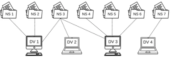
First, the previously mentionednamespaces per device component specifies

how many namespaces devices register. Second, a namespace is visible by a

number of devices, characterized by thedevices per namespacecomponent. This

scheme is represented in Figure 4, in which seven namespaces and four devices are depicted. Namespaces and devices have a many-to-many relationship, where each namespace is associated with at least one device and vice-verse.

When a device starts a new session, it first retrieves all updates in shared namespaces while it has been off-line. For instance, if a device has shared fold-ers with third-parties, all pending updates in those shared foldfold-ers are retrieved. This behavior is represented in Figure 3, in which we can see downloads happen-ing when sessions start. Whenever a device uploads content to a namespace, the content propagation network is consulted to schedule content propagation. All peer devices that are on-line retrieve the updates immediately, whereas off-line devices are scheduled to update when their current inter-session time expires.

Figure 4: Example of the content propagation network (DV stands for device).

In sum, our Dropbox client model has several components. At the highest session layer, client behavior is represented in terms of session duration and inter-session time. At the namespace layer, the model captures the modifica-tions in namespaces by selecting a number of namespaces in each session and using the number of modifications and the inter-modification time to schedule modifications. Modifications are propagated by consulting the content propaga-tion network. Finally, at the lowest data transmission layer, modificapropaga-tions are represented by the upload volume they produce. Next, we characterize these components from empirical data.

4.3. Characterization

We characterize each component presenting the statistical distribution that best fits our measurements. We focus only on the working days in our data, removing all activity observed during weekends or holidays, since we do not model such seasonality.

Best-fitted distributions are determined by comparing our data to fitted curves for a number of models [18]: (i) Normal, Log-normal, Exponential, Cauchy, Gamma, Logistic, Beta, Uniform, Weibull and Pareto, for continu-ous variables; and (ii) Poisson, Binomial, Negative Binomial, Geometric and Hypergeometric, for discrete variables. The Maximum-Likelihood Estimation (MLE) method [18] is used to estimate distribution parameters. We use the Kolmogorov-Smirnov statistic [19] for comparing our sample to continuous dis-tributions and the Least Square Errors [20] for discrete disdis-tributions.

We summarize results next, while Probability Density Functions (PDFs) and parameters of the best-fitted distributions are listed in Appendix A. De-spite variations in the estimated parameters, explained by differences in usage scenarios, the same distributions have been found for each component in the four datasets. These results suggest our model captures, at a good extent, the generic functioning of the Dropbox client.

4.3.1. Session Layer Session Duration:

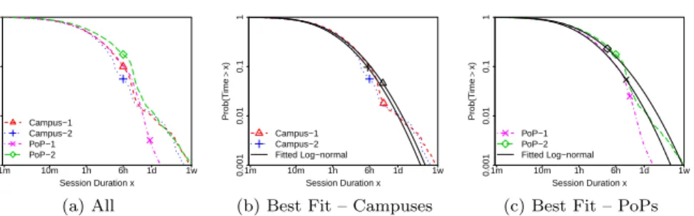
Figure 5 describes sessions duration by plotting the empirical Complemen-tary Cumulative Distribution Functions (CCDFs) for each dataset. Figure 5a contrasts the datasets, whereas Figures 5b and 5c show separate plots for cam-puses and PoPs, including lines for the best-fitted distributions.

Session Duration x Prob(T im e > x) 1m 10m 1h 6h 1d 1w 0.001 0.01 0.1 1 Campus−1 Campus−2 PoP−1 PoP−2 (a) All Session Duration x Prob(T im e > x) 1m 10m 1h 6h 1d 1w 0.001 0.01 0.1 1 Campus−1 Campus−2 Fitted Log−normal

(b) Best Fit – Campuses

Session Duration x Prob(T im e > x) 1m 10m 1h 6h 1d 1w 0.001 0.01 0.1 1 PoP−1 PoP−2 Fitted Log−normal

(c) Best Fit – PoPs Figure 5: Session duration. Note the logarithmic axes. Distributions are similar in different scenarios despite differences in the tails. The best fitted distribution is always Log-normal.

Focusing on Figure 5a, note how the majority of Dropbox sessions are short. The duration follows similar patterns in all datasets – e.g., at least 42% of the sessions are shorter than one hour. However, we observe that sessions are slightly shorter in campuses and PoP-1 than in PoP-2. Indeed, 90% of the sessions in campuses and in PoP-1 are under 6 hours, whereas 90% of the sessions in PoP-2 last up to 9 hours. This can be explained by the sole presence of FTTH users in PoP-2. Our results suggest that FTTH users tend to enjoy longer on-line periods than others. Note also how the number of very long sessions is smaller in PoP-1, where ADSL lines seem to provide less stable connectivity to users.

Despite the variations, we find that the Log-normal distribution describes well the data from all sites. Interestingly, Log-normal distributions have been used to model client active periods in other systems, such as in Peer-to-Peer [21]. Inter-Session Time:

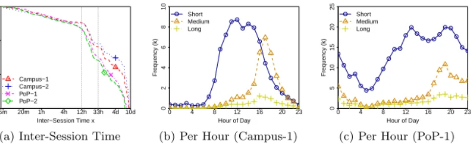
In contrast to sessions duration, we find much higher variability in inter-session times. Our data suggest that inter-inter-sessions are characterized by a mix of distributions that hardly fits well a single model. Intuitively, this happens due to the routine of users in working days in different environments, which includes short breaks during the day and long breaks overnight or across days. Moreover, we clearly notice the existence of classes of users, as previously suggested in [1]. Only a small portion of devices (20–40%) connects daily to Dropbox, while the remaining ones are seen only occasionally.

These patterns are illustrated in Figure 6a, which depicts CCDFs of inter-session times in the four datasets (note the logarithmic scales). We see a

major-ity ofshort inter-sessions (67–76%) that are shorter than 12 hours, compatible

with intraday breaks. A significant percentage ofmedium inter-sessions (20–

28%) lasts between 12 and 33 hours. Those define primarily the overnight off-line intervals of devices that connect to Dropbox every day (i.e., frequent

Inter−Session Time x Prob(T im e > x) 5m 20m 1h 4h 12h 33h 4d 10d 0.001 0.01 0.1 1 Campus−1 Campus−2 PoP−1 PoP−2

(a) Inter-Session Time

0 2 4 6 8 10 Hour of Day Frequency (k) 0 4 8 12 16 20 23 Short Medium Long

(b) Per Hour (Campus-1)

0 5 10 15 20 25 Hour of Day Frequency (k) 0 4 8 12 16 20 23 Short Medium Long

(c) Per Hour (PoP-1) Figure 6: Typical ranges composing the inter-session time distribution and the frequency we observe each range per time of the day in Campus-1 and PoP-1.

hours (≈5%) appears in the tails of the distributions, characterizing long breaks

of occasional devices.6

Interestingly, the intraday routine in each environment determines when inter-session ranges appear in practice. Figures 6b and 6c depict the frequency we observe each range in Campus-1 and PoP-1, respectively, considering the time of the day inter-sessions start. We can see that short inter-sessions are more common between 8:00 and 18:00 in Campus-1, but between 8:00 and 23:00 in PoP-1. Medium and long inter-sessions peak in the evenings in both cases, when devices disconnect to return next day (frequent) or some days later (occasional). We opt for breaking the measurements into three ranges to determine the best-fitted distributions. We also vary the probability of observing each range when generating workloads in Section 5, considering the existence of frequent and occasional devices and the probability of each range throughout the day.

Figure 7 shows CCDFs with respective best fits for each inter-session range in Campus-1 and PoP-1. We observe similar behavior for CCDFs of Campus-2 and PoP-2. Log-normal is the best choice for all datasets in the three ranges. However, note how long inter-sessions present peculiar curves, pointing again to a complex process that is hard to be described with a simple model. Even if fits are not tight for this range, it has little impact on generated workloads, thanks to the low frequency (5%) long inter-sessions occur in practice.

4.3.2. Namespace Layer Namespaces per Device:

Figure 8a shows the CCDF of the number of namespaces per device. Results are in-line with findings in [1]. The number of devices with a single namespace is small: around 10–22% in campus networks, and 25–35% in residential networks. Devices in campuses as well as those of users enjoying fast Internet

connectiv-6_{Note that we ignore inter-sessions longer than 10 days to reduce effects of seasonality.}

Inter−Session Time x Prob(T im e > x) 5m 16m 1h 4h 12h 0.001 0.01 0.1 1 Campus−1 PoP−1 Fitted Log−normal (a) Short Inter−Session Time x Prob(T im e > x) 12h 17h 24h 33h 0.001 0.01 0.1 1 Campus−1 PoP−1 Fitted Log−normal (b) Medium Inter−Session Time x Prob(T im e > x) 33h 3d 6d 10d 0.001 0.01 0.1 1 Campus−1 PoP−1 Fitted Log−normal (c) Long Figure 7: Inter-session times per range and best-fitted Log-normal distributions.

Namespaces per Device x

Prob(N a mespa ces > x) 1 2 4 8 16 32 64 0.001 0.01 0.1 1 Campus−1 Campus−2 PoP−1 PoP−2 (a) All

Namespaces per Device x

Prob(N a mespa ces > x) 1 2 4 8 16 0.001 0.01 0.1 1 Campus−1 Campus−2 PoP−1 PoP−2 (b) Per Week

Namespaces per Device x

Prob(N a mespa ces > x) 1 2 4 8 16 0.001 0.01 0.1 1 Campus−1 Campus−2 Fitted Neg. Binomial

(c) Best Fit – Campuses Figure 8: Namespaces per device considering all namespaces (a) and only those modified in 1-week long intervals (b) with best fits in campuses (c). Note differences inx-axes.

ity at home have higher number of namespaces. Compare the line for PoP-2 (FTTH) with the one for PoP-1 (FTTH and ADSL) in the figure.

We however notice the existence of temporal locality when users modify namespaces. Indeed, although the number of namespaces per device is usually high, users tend to keep working on few namespaces in short time intervals. This effect is illustrated in Figure 8b, in which we plot the distribution of the number of namespaces per device, considering only namespaces that have at least one modification in arbitrary 1-week long intervals of our datasets, and ignoring devices with no modifications. We can see that most devices among those that have modifications produce new workloads in a single namespace in a full week (i.e., 40–53% in campuses and 56–66% in PoPs), while 80% of the devices modify no more than 3 (campuses) or 2 (PoPs) namespaces per week.

Since we are interested in the workload in short time intervals (i.e., weeks), we refrain from modeling the temporal locality of namespaces. For the practical proposal of generating workload, we compute the number of namespaces per device based on namespaces for which we observe modifications in one week pe-riods, as in Figure 8b. Despite distinct patterns between campus and residential networks, Figure 8c shows that Negative Binomial distributions are the best fit

Number of Modifications x Prob(Mo d if ica tio n s > x) 1 10 100 1000 0.001 0.01 0.1 1 Campus−1 Campus−2 PoP−1 PoP−2 (a) All Number of Modifications x Prob(Mo d if ica tio n s > x) 1 10 100 1000 0.001 0.01 0.1 1 Campus−1 Campus−2 Fitted Pareto Type II

(b) Best Fit – Campuses

Number of Modifications x Prob(Mo d if ica tio n s > x) 1 10 100 1000 0.001 0.01 0.1 1 PoP−1 PoP−2 Fitted Pareto Type II

(c) Best Fit – PoPs Figure 9: Number of modifications. Pareto Type II distributions are the best candidate.

in campus datasets. PoP datasets are omitted for the sake of brevity, but they provide the same conclusion.

Namespace Selection:

We derive the methodology to select which namespaces upload content dur-ing a session. We find that the vast majority of sessions (85–93%) have no uploads at all. Clients connect to Dropbox servers, check for possible updates, but do not modify any files locally, i.e., they do not upload content. The re-maining sessions typically have modifications in a single namespace, with less than 2% of the sessions experiencing changes in multiple namespaces. This is expected, since the temporal locality implies that each namespace is changed in restrict periods of time.

Thus, for simplicity, we determine whether a session will see modifications

by computing the probability of modifications inany namespaces (e.g., 15% in

Campus-1 and 7% in PoP-1). Then, we select a random namespace for each session that has modifications.

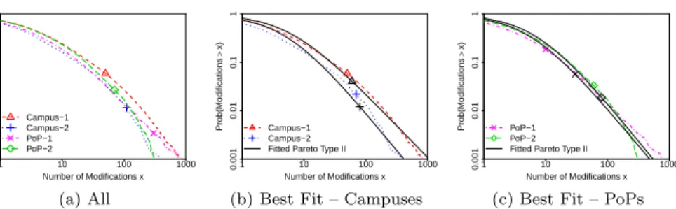
Number of Modifications:

We characterize the 7–15% of sessions that have at least one modification in namespaces. Figure 9 shows CCDFs of the number of modifications per session. In general, users make few modifications in namespaces per session. Fig-ure 9a shows that, among sessions that have at least one modification, around 26% have a single modification, whereas 75% of them have no more than 10 modifications. However, we also observe a non-negligible number of sessions with lots of modifications. Focusing on the tail of the distributions in Fig-ure 9a, notice that around 2% of the sessions have more than 100 modifications. Such heavy tailed distributions are well characterized by Pareto models. Indeed, we can see in Figures 9b and 9c that Pareto Type II distributions fit our data satisfactorily, despite differences in parameters per dataset.

Inter-Modification Time:

Figure 10 shows CCDFs for inter-modification times, which are computed considering sessions with at least two modifications.

Inter−Modification Time x Prob(T im e > x) 1s 10s 2m 1h 1d 0.001 0.01 0.1 1 Campus−1 Campus−2 PoP−1 PoP−2 (a) All Inter−Modification Time x Prob(T im e > x) 1s 10s 2m 1h 1d 0.001 0.01 0.1 1 Campus−1 Campus−2 Fitted Log−Normal

(b) Best Fit – Campuses

Inter−Modification Time x Prob(T im e > x) 1s 10s 2m 1h 1d 0.001 0.01 0.1 1 PoP−1 PoP−2 Fitted Log−Normal

(c) Best Fit – PoPs Figure 10: Inter-modification time. Log-normal distributions are the best candidate.

Figure 10a shows that short time intervals are frequent between modifica-tions. For instance, at least 60% of the inter-modification times are shorter than 1 minute in all sites. This indicates that namespaces tend to present bursts of modifications. Indeed, sessions with large numbers of modifications are char-acterized by such bursts. However, we also observe inter-modification times of hours, which seems to represent the interval between bursts in long-lived ses-sions. The combination of inter- and intra-burst intervals result in distributions that are strongly skewed towards small values. As we can see in Figures 10b and 10c, which depict CCDFs together with the best fits, Log-normal distribu-tions describe our data best.

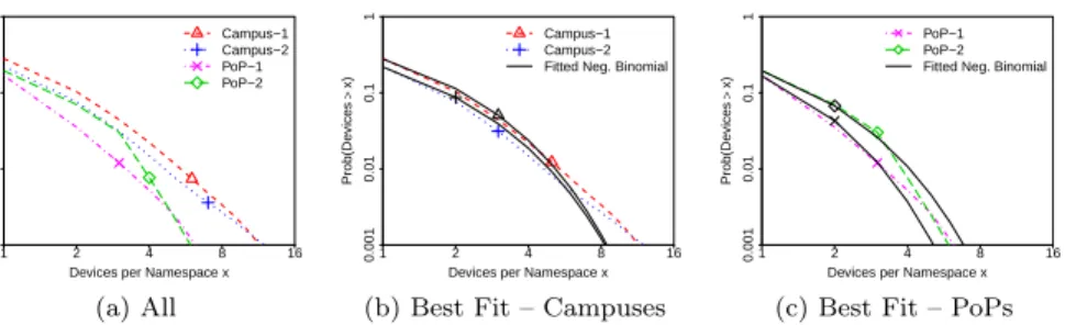
Devices per Namespace:

The last component of the namespace layer characterizes how many devices have access to each namespace. Our data provide the means to estimate the number of devices per namespace for the user population in the networks we monitor. Namespaces may have higher number of devices thanks to devices connected outside the studied networks. Thus, our characterization provides a lower-bound for the actual number of devices per namespace.

Figure 11a shows CCDFs of the number of devices per namespace computed for four networks. In contrast to the number of namespaces per device, devices

per namespace doesnot vary greatly when observing all namespaces registered

in the devices or only those users actually modify in a limited time interval – i.e., it is not affected by the temporal locality of namespaces. Thus, results in the figure are computed based on all namespaces observed in each dataset.

We find that the number of devices per namespace in campuses is higher than in PoPs: 33–36% of namespaces are shared by multiple local devices in campuses, whereas that percentage is 24–26% in PoPs. Moreover, the probabil-ity of observing a namespace with a very high number of devices in campuses is slightly greater than in residential networks (see Figure 11a). This is some-how expected, since we have already ssome-hown that devices at campuses have more namespaces than devices at home (recall Figure 8a).

To understand these differences further, we analyze the number of devices per namespace considering which users own the devices – i.e., disregarding devices

Devices per Namespace x Prob(De vi ces > x) 1 2 4 8 16 0.001 0.01 0.1 1 Campus−1 Campus−2 PoP−1 PoP−2 (a) All

Devices per Namespace x

Prob(De vi ces > x) 1 2 4 8 16 0.001 0.01 0.1 1 Campus−1 Campus−2 Fitted Neg. Binomial

(b) Best Fit – Campuses

Devices per Namespace x

Prob(De vi ces > x) 1 2 4 8 16 0.001 0.01 0.1 1 PoP−1 PoP−2 Fitted Neg. Binomial

(c) Best Fit – PoPs Figure 11: Devices per namespace (logarithmic scales). Most namespaces are accessed by a single device in the network. Negative Binomial distributions best fit our data.

of the same user. We observe about 17% of namespaces are shared by multiple local users in campuses, whereas that percentage is 7–8% in PoPs. Thus, the percentage of namespaces registered in devices of different users is much lower in residential networks. These results reinforce that content sharing is more important in the academic scenario, where a more consistent community of users is aggregated. Our residential datasets, instead, capture a scenario in which multiple devices of few users in a household are synchronized.

Despite differences in parameters, we find that Negative Binomial distribu-tions are the best fit for the number of devices per namespace in all sites, as we show in Figure 11b and Figure 11c.

4.3.3. Data Transmission Layer

Finally, we study the volume of upload workloads. We characterize the vari-able using only the subset of notifications for which we have very high confidence about the upload volume – i.e., those notifications that occur while a single de-vice is performing uploads to a single namespace (see Figure 2a in Section 3). We expect to select a random subset of notifications, thus providing a good estimation for the size of each workload.

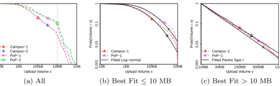
Figure 12a shows CCDFs of upload sizes. Interestingly, uploads are larger in PoPs than in campuses. We conjecture that this happens because users at home often rely on cloud storage for backups and for uploading multimedia files, while a high number of small uploads is seen in campus due to interactive work. The figure clearly shows knees in the distributions at around 10 MB for all datasets. Uploads with volume under 10 MB are the majority, e.g., 97% and 89% in Campus-1 and PoP-1, respectively. This can be explained by two factors. First, the Dropbox client aggregates multiple small files in batches, committing transactions at arbitrary batch sizes to start content propagation while processing other files [1]. This strategy may bias workload sizes towards particular thresholds (e.g., 10 MB). Second, it has already been shown that file sizes in general are not modeled well by a single distribution model, with the body and the tail of the empirical distribution following distinct processes [22].

Upload Volume x Prob(V o lume > x) 10B 1kB 100kB 10MB 1GB 0.001 0.01 0.1 1 Campus−1 Campus−2 PoP−1 PoP−2 (a) All Upload Volume x Prob(V o lume > x) 10B 1kB 100kB 10MB 0.001 0.01 0.1 1 Campus−1 PoP−1 Fitted Log−normal (b) Best Fit≤10 MB Upload Volume x Prob(V o lume > x) 10MB 30MB 100MB 300MB 1GB 0.001 0.01 0.1 1 Campus−1 PoP−1 Fitted Pareto Type I

(c) Best Fit>10 MB

Figure 12: Upload volumes. Data are best-fitted by different models at the body (Log-normal) and at the tail (Pareto Type I). Uploads at PoPs are larger than in campuses.

This suggests to break the measured data into two ranges, determining the best fit for each range independently. Figure 12b shows the empirical distribu-tions and best fits for the measured volumes up to 10 MB, whereas Figure 12c shows curves for the volumes greater than 10 MB. Only Campus-1 and PoP-1 are shown to improve visualization. In all datasets, Log-normal distributions are the ones that better describe our data up to 10 MB (see Figure 12b). On the other hand, uploads with volume greater than 10 MB are best fitted by the Pareto Type I distribution (see Figure 12c). Interestingly, these results are in agreement with the generative model for file sizes proposed in [22].

5. CloudGen– Cloud Storage Traffic Generator

5.1. Overview

We implement CloudGen based on our hierarchical model for the Drop-box client. CloudGen receives as input parameters for the set of distributions characterizing the model, as well as execution parameters, such as the synthetic

workload duration and the target number of devices (d). The latter can be freely

set to determine the population size to be evaluated. As outcome, CloudGen produces a synthetic trace indicating when each device is active and inactive, the series of modifications in namespaces, and the data volume of modifications. Therefore, we envisage the use of CloudGen in a variety of scenarios, e.g., to evaluate the traffic users in a network produce, or to estimate the workload servers in a cloud storage data-center face in different deployments.

CloudGen starts by setting up the content propagation network, i.e., the structure that represents how namespaces are shared among devices (see Fig-ure 4). This process follows two steps. First, CloudGen derives the number

of distinct namespaces (n) from the number of devices (d), using the mean

number of namespaces per device (nd) and the mean number of devices per

namespace (dn), both coming from distributions characterized in Section 4.3.2.

The expected number of distinct namespaces is given byn=d×nd/dn. As an

example, our data provide an average ratio of distinct namespaces per device

Second, CloudGen associates devices to namespaces. For that, CloudGen includes a method to generate random networks based on [23]: (i) CloudGen first picks one namespace for each device to make sure all devices have at least one namespace; then (ii) it complements the number of devices of each namespace (sampled from the distribution of devices per namespace), by selecting random devices with the probability proportional to the number of namespaces in the devices (sampled from the distribution of namespaces per device).

CloudGen then generates workloads following a classic discrete-event simu-lation approach. First, it creates a sequence of events to mark session logins and logouts of each device. The time of each event is determined by sampling the sessions duration and the inter-session time distributions, until the next login of all devices falls outside the synthetic trace duration.

To compute inter-session times, CloudGen samples from the inter-session ranges (i.e., short, medium or long) based on their probabilities throughout the day. However, CloudGen separates devices into two groups (frequent and occasional), and enforces only medium inter-sessions (frequent devices) or long inter-sessions (occasional devices) in night periods. As such, CloudGen mimics the behavior shown in Figure 6, which results in a sharp decrease in the number of new sessions at night, and multiple-day breaks for occasional devices. Note that while CloudGen captures intraday variations, thanks to the procedure to select inter-session times, other seasonal patterns (e.g., weekly or yearly) are intentionally left out for the sake of simplicity.

For each session, CloudGen decides whether new events are required by fol-lowing our namespace selection strategy: First, it evaluates the probability that any namespaces in the session are modified. When modifications should occur, CloudGen randomly selects a namespace to execute modifications. CloudGen then determines how many modifications to place in the session. It does so by following a method found on [24] to match the distribution of sessions duration with the distribution of the number of modifications per session. Basically, the longer sessions are, the higher are the chances they experience lots of modifica-tions. Then, the series of modification events is scheduled using the distribution of inter-modification times in a best-effort fashion: Samples of inter-modification times determine the time of the next modification in the session; if the session duration is reached before scheduling all modifications, the remaining modifica-tions are scheduled starting from the session begin again.

CloudGen assigns the upload volume to each modification and, eventually, schedules download events using the content propagation network and the infor-mation about login and logout times of peer devices. Modifications that happen in a shared namespaces are then propagated to all peer devices. CloudGen is

available as free software athttp://cloudgen.sourceforge.net.

5.2. Validation Methodology:

We validate CloudGen by comparing synthetic and actual traces in Campus-1 and PoP-1 datasets. We first determine the input number of devices.

To remove possible effects of the registration and removal of devices to/from Dropbox, we pick several weeks of data in each dataset and count the num-ber of active devices per week. Then, we execute CloudGen entering the mean number of active devices per week in each dataset, together with the respective distribution parameters characterized in the previous section.

We set CloudGen to generate synthetic traces of two weeks, to make sure all ranges of inter-session times are used in the simulation. Moreover, we discard the initial week to remove simulation warm-up effects, as well as weekends since our model does not include such seasonality. We repeat the procedure sixteen times for each dataset, to obtain different samples of synthetic traces.

We then contrast synthetic traces to Campus-1 and PoP-1 datasets. We

focus on two types of metrics: (i) Direct metrics to validate that synthetic

traces follow the distributions that define our model – e.g., we compute synthetic inter-session times to analyze the impact of simplifications we made to build

CloudGen; (ii)Indirect metrics that are not explicitly encoded in our model –

e.g., we use the aggregated workload devices produce in pre-determined periods (e.g., per day) to check whether synthetic traces approximate well the workload users create to Dropbox.

Direct Metrics:

We recompute all components of our model characterized in Section 4.3, now using synthetic traces, to validate CloudGen implementation. For the sake of brevity, we show results only for Campus-1 in this first test, since PoP-1 leads to the same conclusions. We also omit plots for sessions duration, number of modifications per session, upload volume and devices per namespace, since these variables are used directly by CloudGen, without any specific design decision to simplify implementation.

Figure 13 summarizes metrics for which CloudGen implementation includes simplifications. We depict in each plot the empirical distribution found in actual traces, along with the distribution extracted from the synthetic traces.

Inter-sessions times are depicted in Figures 13a. We can see that synthetic and actual distributions are tightly close to each other. Synthetic traces present the three-range pattern seen in actual data, with correct proportions among the ranges. Thus, we can conclude that our strategy to split devices as frequent and occasional, as well as to select inter-session ranges, works well in practice.

Figure 13b depicts inter-modification times. Since inter-modification times are used only to distribute modifications in the sessions, and we adopt heuris-tics to match the number of modifications and the sessions duration, inter-modification times are prone to errors due to simplifications in our method. In-deed, synthetic traces present slightly more short inter-modification times than the actual ones. Still, the artifact affects less than 10% of the measurements, noticeable in the tail of distributions.

Finally, Figure 13c presents the number of namespaces per device, which is used indirectly as a weight when sampling devices for the content propagation network. We can see that synthetic and actual traces slightly diverge in the tail of the distributions. This difference is, however, compatible with the distribution

Inter−Session Time x Prob(T im e > x) 5m 20m 1h 4h 12h 33h 4d 10d 0.001 0.01 0.1 1 Actual Synthetic

(a) Inter-Session Time

Inter−Modification Time x Prob(T im e > x) 1s 10s 2m 1h 1d 0.001 0.01 0.1 1 Actual Synthetic (b) Inter-Modification Time

Number of Namespaces per Device x

Prob(N a mesp a ce s > x) 1 2 4 8 16 0.001 0.01 0.1 1 Actual Synthetic

(c) Namespaces per Device Figure 13: Comparison of model components in actual and synthetic traces in Campus-1.

characterized for the variable. In fact, our method to create content propagation networks approximates well both distributions that characterize the Dropbox network, even when small networks are created (e.g., hundreds of devices).

Overall, we conclude that our implementation is satisfactory and produces synthetic traces similar to datasets used as input to our model.

Indirect Metrics:

Next we validate CloudGen focusing on three indirect metrics: the number of sessions, the number of modifications in namespaces and the total upload volume. We compute the metrics after aggregating the activity of all devices per day. Such metrics summarize the overall workload the network and servers need to handle in a time interval, given a fixed population of devices. Our goal is to understand whether CloudGen realistically reproduces the metrics when it is fed with the number of devices seen in actual traces.

Figure 14 presents CDFs for the indirect metrics. Top plots are relative to Campus-1, while bottom plots depict results for PoP-1.

Figure 14a and 14d show that the number of sessions per day in synthetic traces is relatively close to actual values. Focusing on Figure 14d, note how the synthetic distribution captures the overall trend in actual data for PoP-1. Mean values for synthetic and actual traces are 4,542 and 4,551 in PoP-1, respectively. The number of sessions per day is slightly off actual values in Campus-1: mean of 5,649 for the synthetic trace and 5,219 for the actual one (i.e., synthetic overestimates by 8%), and we see more variability in actual traces. This happens because, for the sake of simplicity, CloudGen generates similar workloads for all weekdays, while campus routine clearly varies during the week – e.g., fewer devices are typically seen active on Wednesdays and Fridays in Campus-1. Thus, in environments with very high mobility of users, such as in campus networks, CloudGen approximates well mean values, but smooths the number of sessions per day.

Figures 14b and 14e show distributions for the number of modifications per day. Synthetic traces follow the overall trend in actual data again, in particular regarding mean values. The mean numbers of modifications per day are 14,174 (synthetic) and 13,884 (actual) in Campus-1 (synthetic overestimates by 2%),

0 2 4 6 8 10 0.0 0.2 0.4 0.6 0.8 1.0 Number of Sessions (k) x Prob(Nu mbe r ≤ x) Actual Synthetic

(a) Number of Sessions

0 10 20 30 40 0.0 0.2 0.4 0.6 0.8 1.0 Number of Modifications (k) x Prob(Nu mbe r ≤ x) Actual Synthetic (b) Number of Modifications 0 10 20 30 40 50 60 0.0 0.2 0.4 0.6 0.8 1.0 Upload Volume (GB) x Prob(V o lume ≤ x) Actual Synthetic (c) Upload Volume 0 2 4 6 8 0.0 0.2 0.4 0.6 0.8 1.0 Number of Sessions (k) x Prob(Number ≤ x) Actual Synthetic (d) Number of Sessions 0 2 4 6 8 10 0.0 0.2 0.4 0.6 0.8 1.0 Number of Modifications (k) x Prob(Number ≤ x) Actual Synthetic

(e) Number of Modifications

0 5 10 15 20 25 30 35 0.0 0.2 0.4 0.6 0.8 1.0 Upload Volume (GB) x Prob(V o lu me ≤ x) Actual Synthetic (f) Upload Volume Figure 14: CDFs of indirect metrics (per day) for synthetic and actual traces in Campus-1 (1st. row) and PoP-1 (2nd. row). CloudGen slightly overestimates the workload.

and 4,286 (synthetic) and 4,530 (actual) in PoP-1 (synthetic underestimates by 5%). Although mean values are closer in Campus-1 than in PoP-1, more variability can be noticed in Campus-1 in Figure 14b, once more, thanks to the heterogeneous users’ routine in the environment throughout the week.

Figures 14c and 14f show distributions for the total upload volume per day in Campus-1 and PoP-1, respectively. We can see that CloudGen overestimates the upload volume per day. Mean volumes per day are 22 GB (synthetic) and 20 GB (actual) in Campus-1 (synthetic overestimates by 10%), and 14 GB (syn-thetic) and 13 GB (actual) in PoP-1 (synthetic overestimates by 8%). Synthetic mean volumes are slightly higher than actual mean volumes, despite the visual similarity of the distributions in the figures, due to the tails of the synthetic volumes – i.e., few days with very high workloads in synthetic traces. Yet, synthetic values are very close to the actual ones.

We conclude that synthetic workloads capture the main trends in actual traces. CloudGen provides conservative estimates of the upload traffic of a pop-ulation of devices, because of the heavy tailed Pareto distributions character-ized for the number and volume of uploads. CloudGen reconstructs reasonably well the aggregated workload in typical campus and residential networks, even though its design is based on a per-client workload model, which is challenge for a complex system as Dropbox. CloudGen is a valuable tool, helping admin-istrators to easily provision resources for cloud storage services.

6. Future Scenarios for Cloud Storage Usage

6.1. Scenarios

Our goal is to obtain insights on the traffic volume in near future scenarios where, due to the increasing popularity of cloud storage, we will see a larger number of users adopting such services, more devices being registered and, even-tually, more content sharing through shared namespaces. We define three sce-narios to explore how network traffic would behave with those trends:

1. Larger Population: This scenario studies how Dropbox user population growth affects network traffic. We increase the number of devices, eval-uating how the network traffic changes with up to 10-times more devices

than what is observed nowadays in edge networks.7

2. Larger Sharing: We simulate a scenario where users share more content through cloud storage. We achieve that by increasing the mean number of devices per namespace. More precisely, we manually determine the

param-eterrof the Negative Binomial distribution (see Appendix A) that leads

to the desired mean number of devices per namespace of each experiment. 3. Larger Population and Sharing: We combine the previous two scenarios, to simulate a future where more devices are registered to Dropbox, while users also become more prone to share content.

All remaining CloudGen parameters are kept constant in each scenario. We present results for CloudGen parameterized with Campus-1 and PoP-1 distri-butions only, since other datasets result in similar conclusions. We perform 16 experiment rounds for each configuration, recording upload and download vol-umes. We compute the metrics for a one-week long interval, after discarding CloudGen warm-up period and weekends. Finally, for the sake of simplicity, we assume a static and closed population of devices in these experiments: devices never leave the simulated environment, all uploaded content is propagated in the local network and external devices produce no workload.

6.2. Traffic Analysis

Figure 15 presents mean upload and download volumes as number of devices is varied (larger population scenario). Error bars mark 95% confidence intervals. We can see that upload and download volumes grow roughly linearly with the number of devices in the network – e.g., note how there are around twice as much upload when doubling the device population in both Campus-1 and PoP-1. Interesting, the download volume is greater than the upload one in Campus-1, whereas the opposite pattern is observed in PoP-1. Moreover, download volume grows slower than the upload volume with PoP-1 parameterization. This hap-pens because a higher number of devices per namespace is observed in Campus-1 than in PoP-1 (Section 4.3.2). Thus, uploads in the campus more likely trigger

0.0 0.5 1.0 1.5 2.0 Increase (devices) V olume (TB) 1 2 3 4 5 6 7 8 9 10 Upload Download (a) Campus-1 0.0 0.5 1.0 1.5 2.0 Increase (devices) V olume (TB) 1 2 3 4 5 6 7 8 9 10 Upload Download (b) PoP-1

Figure 15: Mean upload and download volumes in larger population scenarios.

0.0 0.5 1.0 1.5 2.0 Increase (sharing) V olume (TB) 1 2 3 4 5 6 7 8 9 10 Upload Download (a) Campus-1 0.0 0.5 1.0 1.5 2.0 Increase (sharing) V olume (TB) 1 2 3 4 5 6 7 8 9 10 Upload Download (b) PoP-1

Figure 16: Mean upload and download volumes in larger sharing scenarios.

several downloads. Overall, we conclude that the network traffic of larger device populations can be trivially estimated, provided that sharing behavior of users is known and remains constant as the population increases.

Figure 16 presents mean traffic volumes for the larger sharing scenario – i.e., when we increase only the mean number of devices per namespace. Natu-rally, varying the number of devices per namespace does not affect the upload. Download volume, on the other hand, is strongly affected by the parameter. We observe that the download volume more than double when doubling the mean number of devices per namespace for both Campus-1 and PoP-1. For instance, mean download volumes are 0.1, 0.3, 0.6 and 1.4 TB in Campus-1 when the respective mean number of devices per namespace is 1, 2, 4 and 8 times the values observed in actual traces. Similar trend can be noted for PoP-1.

Finally, Figure 17 presents the larger population and sharing scenario, in which we vary both the number of devices and the mean number of devices per

0

5

10

15

20

Increase (devices and sharing)

V olume (TB) 1 2 3 4 5 6 7 8 9 10 Upload Download (a) Campus-1 0 5 10 15 20

Increase (devices and sharing)

V olume (TB) 1 2 3 4 5 6 7 8 9 10 Upload Download (b) PoP-1

Figure 17: Mean upload and download volumes in larger population and sharing scenarios.

namespace simultaneously. For this figure, we increase both quantities at the same rate. Upload volume follows the trend observed in Figure 15 as expected. More interesting, note how this combination of more devices with more sharing results in a quadratic-like growth in download traffic. For instance, when both the number of devices and the mean number of devices per namespace are 1, 2, 4 and 8 times the values observed in actual traces, the mean download volumes are 0.1, 0.7, 3.0 and 15.7 TB in Campus-1 and 0.05, 0.3, 1.5 and 5.6 TB in PoP-1, respectively. That is, in a hypothetical scenario where there are four times more devices than what is observed nowadays, and where those devices share 4 times more namespaces, edge networks would experience up to a 30-fold increase in the download traffic related to cloud storage.

This simple study shows the effectiveness of CloudGen for evaluating future cloud storage usage scenarios.

7. Related Work

This work studies theunderlying client processesin cloud storage services. In

particular, we extend our preliminary work presented in [10], which introduces a hierarchical model for the Dropbox client behavior, and in [11], which presents a preliminary implementation of CloudGen. Our extended model captures content modifications that lead to data exchanges in the network. It also describes how content is propagated in the Dropbox network of shared folders and among the several devices of a user. We build upon our model to develop and validate a workload generator for cloud storage using data collected in four different networks. Finally, we apply CloudGen to evaluate the expected growth of cloud storage traffic in edge networks.

In the following, we summarize other related work, discussing both efforts that address aspects of cloud storage services (Section 7.1) and efforts to model and evaluate workloads of Internet services in general (Section 7.2).

7.1. Cloud Storage Services

Cloud storage services have received large attention from the research com-munity. Drago et al. [1] are the first to present an in-depth characterization of typical usage and performance bottlenecks of Dropbox from passive measure-ments. We partly rely on their methodology to collect and process data about Dropbox. Unlike [1], and motivated by our model for the Dropbox client behav-ior, we characterize Dropbox workload taking into account users’ sessions and content sharing. Moreover, we leverage the characterization to build a workload generator and to evaluate possible future scenarios for Dropbox usage.

Various studies focus on benchmarking cloud storage using active experi-ments. Hu et al. [25] study the backup performance of four services. Wang et al. [26] analyze Dropbox bottlenecks, while the public APIs of three providers are compared in [9]. Authors of [3] introduce a framework to benchmark cloud storage. Relying on an automated testing methodology, they compare design choices and implications by benchmarking 11 services. Li et al. [8] follow a similar methodology and compare cloud storage performance considering also different types of client terminals. None of them characterize or model the behavior of actual cloud storage users, as we do in this work.

Some works propose alternative protocols and architectures to improve per-formance or to decrease costs of cloud storage services. In [27], a framework that collects semantic information from files (e.g., file type) is proposed to improve performance of the services. Zhang et al. [5] propose a mechanism to ensure con-sistency between the local file system and remote repositories. Authors of [4] propose QuickSync, a system that optimizes synchronization by combining novel techniques, such as network-aware chunking. Our work contributes to such ef-forts with a workload generator that can be used to evaluate new proposals in realistic scenarios.

Finally, other works analyze cloud storage focusing on economics, security, quality of experience or privacy, and thus are orthogonal to our work. For exam-ple, authors of [28] compare pricing practices in the storage market. Mulazzani et al. [14] uncover security issues related to the storage of content in the cloud. Quality of experience of storage services is studied in [6, 7], while the type of files people store in the cloud are evaluated in [29].

7.2. Models and Workload Generators for Internet Services

To the best of our knowledge, we are the first to propose a model and to implement and validate a system to generate synthetic workloads for cloud storage services, such as Dropbox.

Several models and workload generators have been proposed to create web request streams [24, 30–32]. Two of them model users’ behavior and its impacts on network traffic and, as such, are closer to our work. SURGE [24] is a workload generator that employs the concept of user equivalents to generate traffic for web servers. SWAT [32] considers user sessions and the dependence of content requests within sessions. We borrow general ideas from SURGE, such as to